Fundamental Quantum Limit to Waveform Estimation

Abstract

We derive a quantum Cramér-Rao bound (QCRB) on the error of estimating a time-changing signal. The QCRB provides a fundamental limit to the performance of general quantum sensors, such as gravitational-wave detectors, force sensors, and atomic magnetometers. We apply the QCRB to the problem of force estimation via continuous monitoring of the position of a harmonic oscillator, in which case the QCRB takes the form of a spectral uncertainty principle. The bound on the force-estimation error can be achieved by implementing quantum noise cancellation in the experimental setup and applying smoothing to the observations.

The accuracy of any sensor is limited by noise. To quantify the potential performance of a sensor, it is often useful to compute a lower bound to the error in the estimation of the signal of interest. One of the most widely used bounds is the Cramér-Rao bound (CRB), which limits the mean-square error in parameter estimation vantrees .

The development of quantum technology highlights the question of how quantum mechanics impacts the performance of sensors. Helstrom formulated a quantum Cramér-Rao bound (QCRB) helstrom , which stipulates that the minimum estimation error is inversely proportional to a property of the sensor known as the quantum Fisher information. The QCRB is central to quantum sensor design in the burgeoning field of quantum metrology wiseman ; glm for several reasons. It allows one to determine whether the fundamental sensitivity of a sensor design meets the requirements of an application, provides a criterion against which the optimality of quantum sensing schemes can be tested, and motivates improvements of schemes that are suboptimal. For sensors near the fundamental limit, the QCRB can also be used to quantify the trade-off between sensing accuracy and physical resources of the sensor, so that efficient ways of improving sensitivity can be identified.

Most prior work on the QCRB considered estimation of one or a few fixed parameters. Yet, in most sensing applications, such as force sensing and magnetometry, the signal of interest is changing in time. This time-changing signal, which we call a waveform, is coupled continuously to the sensor, and continuous measurements on the sensor are used to extract information about the waveform braginsky ; berry ; smooth . Here we derive the QCRB for waveform estimation—the first such derivation to our knowledge—allowing for any quantum measurement protocol, including sequential, discrete or continuous measurements.

Previous work on the QCRB generally did not take into account prior information, but for the task of estimating a waveform, which often depends on an infinite number of unknown parameters, parameter estimation techniques no longer suffice and prior information is required to make the problem well defined vantrees . The prior information might, for example, restrict the signal to a finite bandwidth, making integrals over frequency finite that otherwise would diverge. Thus a crucial feature of our QCRB is the inclusion of prior waveform information.

Our result provides a rigorous criterion against which the optimality of design, control, and estimation strategies for quantum sensors, such as gravitational-wave detectors, force sensors, and atomic magnetometers, can be tested. As an example, we calculate the QCRB on the error of force estimation via continuous position measurements of a harmonic oscillator, in which case the bound takes the form of a spectral uncertainty principle. We show that the bound can be achieved by implementing quantum noise cancellation (QNC) to remove the backaction noise from the observations qnc and applying the estimation technique of quantum smoothing smooth to the observations. This proves the optimality of such control and estimation techniques for force sensing and establishes our QCRB as the fundamental limit to force sensing.

Let $x(t)$ denote the classical waveform to be estimated. For simplicity, we assume $x(t)$ to be a scalar function; generalization to multiple processes is straightforward. We discretize time as $t_{j}=t_{0}+j\delta t$, $j=0,1,\dots,J$, and assume that $\delta t$ is small enough that we can treat $x(t)$ as piecewise-constant, i.e., $x(t)=x_{j}$ for $t_{j}\leq t<t_{j+1}$. The prior probability density $P[x]$ for the vector $x\equiv(x_{J-1},\dots,x_{0})^{T}$ characterizes what is known or assumed about the waveform prior to the measurements. For a vector of observations $y\equiv(y_{N-1},\dots,y_{1},y_{0})^{T}$ made any time during the interval $t_{0}<t\leq t_{J}$, we define a conditional probability density $P[y|x]$. The joint probability density is $P[y,x]=P[y|x]P[x]$. Finally, we define the estimate of $x_{j}$ as $\tilde{x}_{j}[y]$ and the estimate bias, given signal $x$, as $\int\!Dy\,(\tilde{x}_{j}-x_{j})P[y|x]\equiv b_{j}[x]$, where $Dy\equiv\prod_{n=0}^{N-1}dy_{n}$.

Multiplying both sides of $b_{j}[x]$ by $P[x]$, differentiating with respect to $x_{k}$, and then integrating over all $x$ using $Dx\equiv\prod_{j=0}^{J-1}dx_{j}$, we obtain

$$-\delta_{jk}+\int\!Dx \,Dy\,(\tilde{x}_{j}-x_{j})\frac{\partial P[y,x]}{\partial x_{k}}$$

$$=\int\!Dx\frac{\partial}{\partial x_{k}}\bigl{(}b_{j}[x]P[x]\bigr{)}=0\;,$$ (1)

where the final equality assumes $b_{j}[x]P[x]|_{x_{k}=\pm\infty}=0$. This assumption, also used in the proof of the classical CRB vantrees , is satisfied as long as the prior density approaches zero at the infinite endpoints (as it must for any probability density) and the bias there is not infinite.

Quantum mechanics enters this description, which till now is classical, by determining the conditional probability of the observations. Given a quantum system, we can describe any measurement protocol, including sequential measurements and excess decoherence, during the interval $t_{0}\leq t<t_{J}$ by introducing appropriate ancillae, in accord with the Kraus representation theorem wiseman ; kraus ; nielsen . This also accounts for any feedback during the interval, based on the measurement outcomes, because the principle of deferred measurement nielsen allows one to put off the measurements on the ancillae till time $t_{J}$; measurement-based feedback is replaced by controlled unitaries prior to the measurements, as schematically shown in Fig. 1.

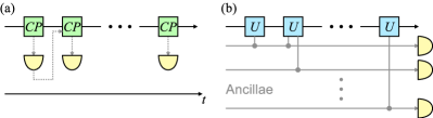
Figure 1: Any quantum dynamics and sequential measurements described by completely positive (CP) maps, including feedback based on measurement outcomes, as illustrated in (a), can be reproduced by unitary evolution of an enlarged system that includes appropriate ancillae, coherent controlled unitaries, and deferred measurements of the ancillae, as shown in (b).

In this approach, the overall system dynamics is described by unitary evolution of the enlarged system; the conditional probability of observations is given by $P[y|x]=\operatorname{tr}\bigl{(}E[y]\rho_{x}\bigr{)}$, where $\rho_{x}$ is the density operator of the enlarged system at time $t_{J}$, conditioned upon $x$, and $E[y]$ is the positive-operator-valued measure (POVM) that describes the (deferred) measurements up to time $t_{J}$. We denote expectation values with respect to $\rho_{x}$ by angle brackets subscripted by $x$, so that $\langle E[y]\rangle_{x}\equiv\operatorname{tr}\bigl{(}E[y]\rho_{x}\bigr{)}$. Continuous measurements can be modeled as the limit of a sequence of infinitesimally weak measurements wiseman .

We now follow a procedure similar to the one used by Helstrom helstrom to derive the QCRB. We introduce an operator $Q_{k}$ that satisfies $\partial\rho_{x}/\partial x_{k}=(Q_{k}\rho_{x}+\rho_{x}Q_{k}^{\dagger})/2$. Unlike Helstrom, we do not require $Q_{k}$ to be Hermitian. Note that the vanishing trace of $\partial\rho_{x}/\partial x_{k}$ in the definition of $Q_{k}$ implies that $\operatorname{Re}\langle Q_{k}\rangle_{x}=0$.

It is convenient to incorporate the prior information by working in terms of a density operator $\rho[x]\equiv\rho_{x}P[x]$ in a hybrid quantum-classical space and introducing an operator $L_{k}=Q_{k}+\partial\ln P[x]/\partial x_{k}$, which satisfies $\partial\rho[x]/\partial x_{k}=(L_{k}[x]\rho[x]+\rho[x]L_{k}^{\dagger}[x])/2$. In terms of $L_{k}$, Eq. (1) takes the form that we use to derive the QCRB:

$$\delta_{jk}=\operatorname{Re}\int\!Dx\,Dy\,(\tilde{x}_{j}-x_{j})\operatorname{tr}\bigl{(}E[y]L_{k}[x]\rho[x]\bigr{)}\;.$$ (2)

Multiplying Eq. (2) by $u_{j}v_{k}$, where $u_{j}$ and $v_{k}$ are the components of arbitrary real column vectors $u$ and $v$, and then summing over all $j$ and $k$, we obtain

$$v^{T}u=\sum_{j}u_{j}v_{j}=\operatorname{Re}\int\!Dx\,Dy\,\operatorname{tr}\!\left(A^{\dagger}B\right)\;,$$ (3)

where $A^{\dagger}\equiv\sum_{k}v_{k}\sqrt{E[y]}L_{k}\sqrt{\rho[x]}$, $B\equiv\sum_{j}u_{j}(\tilde{x}_{j}-x_{j})\sqrt{\rho[x]}\sqrt{E[y]}$, and $T$ denotes transposition. It follows from Eq. (3) that

$$(v^{T}u)^{2} \leq\left|\int\!Dx\,Dy\,\operatorname{tr}\!\left(A^{\dagger}B\right)\right|^{2}$$

$$\leq\int\!Dx\,Dy\,\operatorname{tr}(A^{\dagger}A)\int\!Dx\,Dy\,\operatorname{tr}(B^{\dagger}B)\;,$$ (4)

where the second inequality is the Schwarz inequality.

The second integral in Eq. (4) is $\int\!Dx\,Dy\,\operatorname{tr}(B^{\dagger}B)=u^{T}\Sigma\,u$, where

$$\Sigma_{jk}\equiv\int\!Dx\,Dy\,P[x,y](\tilde{x}_{j}-x_{j})(\tilde{x}_{k}-x_{k})$$ (5)

is the estimation-error covariance matrix. The first integral in Eq. (4) is, using the completeness of the POVM, $\int\!Dx\,Dy\,\operatorname{tr}(A^{\dagger}A)=v^{T}Fv$, where $F$ is a (real, symmetric) Fisher-information matrix,

$$F_{jk}\equiv\frac{1}{2}\int\!Dx\,P[x]\operatorname{tr}\Bigl{(}(L_{j}^{\dagger}L_{k}+L_{k}^{\dagger}L_{j})\rho_{x}\Bigr{)}\;.$$ (6)

Since $\operatorname{Re}\langle Q_{k}\rangle_{x}=0$, $F$ separates neatly into a quantum and a classical, prior-information component, i.e., $F=F^{(Q)}+F^{(C)}$, where

$$F_{jk}^{(Q)} =\frac{1}{2}\int\!Dx\,P[x]\operatorname{tr}\Bigl{(}(Q_{j}^{\dagger}Q_{k}+Q_{k}^{\dagger}Q_{j})\rho_{x}\Bigr{)}$$ (7)

$$F_{jk}^{(C)} =\int\!Dx\,P[x]\frac{\partial\ln P[x]}{\partial x_{j}}\frac{\partial\ln P[x]}{\partial x_{k}}\;.$$ (8)

When these results are substituted into Eq. (4), we find that $(v^{T}Fv)(u^{T}\Sigma u)\geq(v^{T}u)(u^{T}v)$. Setting $v=F^{-1}u$ implies that $u^{T}(\Sigma-F^{-1})u\geq 0$ for arbitrary real vectors $u$. Since $\Sigma-F^{-1}$ is real and symmetric, this implies that $\Sigma-F^{-1}$ is positive-semidefinite; the matrix inequality

$$\Sigma\geq F^{-1}$$ (9)

is the QCRB in its most general form. To use a CRB in practice, it is customary to define a non-negative, quadratic cost function $C\equiv\operatorname{tr}(\Lambda^{T}\Sigma)$ using a positive-semidefinite (Hermitian) cost matrix $\Lambda$ suited to the application vantrees ; helstrom . The matrix QCRB is equivalent to a lower bound, $C\geq\operatorname{tr}(\Lambda^{T}F^{-1})$, on all such cost functions.

To calculate the QCRB, we must be more specific about the evolution of the enlarged quantum system. The Hamiltonian that governs overall system dynamics over the interval $t_{j}\leq t\leq t_{j+1}$, of duration $\delta t$, is $H_{j}(x_{j})$, with corresponding evolution operator $U_{j}=\exp[-iH_{j}(x_{j})\delta t/\hbar]$. We have $\partial U_{j}/\partial x_{j}=U_{j}(-ih_{j}\,\delta t/\hbar)$, where $h_{j}\equiv\partial H_{j}/\partial x_{j}$. Let $U_{kj}\equiv U_{k-1}\cdots U_{j}$ denote the evolution operator over the interval $t_{j}\leq t\leq t_{k}$. The density operator $\rho_{x}$ is related to the initial density operator $\rho_{0}$ by $\rho_{x}=U_{J0}\rho_{0}U^{\dagger}_{J0}$, which gives $\partial\rho_{x}/\partial x_{k}=-i[M_{k},\rho_{x}]$, where

$$M_{k}\equiv i\frac{\partial U_{J0}}{\partial x_{k}}U^{\dagger}_{J0}=\frac{\delta t}{\hbar}U_{Jk}h_{k}U^{\dagger}_{Jk}=\frac{\delta t}{\hbar}U_{J0}\hat{h}_{k}U^{\dagger}_{J0}\;,$$ (10)

with $\hat{h}_{k}\equiv U_{k0}^{\dagger}h_{k}U_{k0}=h(t_{k})$ being the Heisenberg-picture version of $h_{k}$. An obvious choice for $Q_{k}$ is the anti-Hermitian $Q_{k}=-2i\Delta M_{k}$, where $\Delta M_{k}\equiv M_{k}-\langle M_{k}\rangle_{x}$. The quantum part of the Fisher matrix then becomes

$$F_{jk}^{(Q)}\!=\!\frac{4(\delta t)^{2}}{\hbar^{2}}\int\!\!Dx\,P[x]\frac{1}{2}\operatorname{tr}\!\Big{(}(\Delta\hat{h}_{j}\Delta\hat{h}_{k}+\Delta\hat{h}_{k}\Delta\hat{h}_{j})\rho_{0}\Bigr{)}\;,$$ (11)

where $\Delta\hat{h}_{k}\equiv\hat{h}_{k}-\langle\hat{h}_{k}\rangle_{0}$. Angle brackets with subscript 0 denote an expectation value with respect to $\rho_{0}$. The quantum Fisher information is thus a two-time covariance function, averaged over $P[x]$.

To take the continuous-time limit, we let $\delta t\to 0$, $\Sigma_{jk}\to\Sigma(t_{j},t_{k})$, $F_{jk}/(\delta t)^{2}\to F(t_{j},t_{k})$, and $\Lambda_{jk}/(\delta t)^{2}\to\Lambda(t_{j},t_{k})$. The estimation-error covariance matrix becomes the two-time covariance function of estimation error, $\Sigma(t,t^{\prime})$, and the Fisher matrix becomes $F(t,t^{\prime})=F^{(Q)}(t,t^{\prime})+F^{(C)}(t,t^{\prime})$, with

$$F^{(Q)}(t,t^{\prime}) =\frac{4}{\hbar^{2}}\int\!Dx\,P[x]$$

$$\phantom{\int\!}\times\frac{1}{2}\Bigl{\langle}\Delta h(t)\Delta h(t^{\prime})+\Delta h(t^{\prime})\Delta h(t)\Bigr{\rangle}_{\!0}\;,$$ (12)

$$F^{(C)}(t,t^{\prime}) =\int\!Dx\,P[x]\frac{\delta\ln P[x]}{\delta x(t)}\frac{\delta\ln P[x]}{\delta x(t^{\prime})}\;,$$ (13)

$\delta/\delta x(t)$ being the functional derivative.

In the continuous-time limit, the matrix QCRB retains the same form as Eq. (9), where the continuous-time inverse is defined by $\int_{t_{0}}^{t_{J}}dt^{\prime\prime}F(t,t^{\prime\prime})F^{-1}(t^{\prime\prime},t^{\prime})=\delta(t-t^{\prime})$. The bound on a cost function becomes

$$C\equiv\int dt\,dt^{\prime}\,\Lambda(t,t^{\prime})\Sigma(t,t^{\prime})\geq\int dt\,dt^{\prime}\,\Lambda(t,t^{\prime})F^{-1}(t,t^{\prime})\;.$$ (14)

Equation (14), valid for any cost function, is the most serviceable expression of our chief result. An important special case is the point estimation error,

$$\Pi(t)\equiv\Sigma(t,t)=\langle[\tilde{x}(t)-x(t)]^{2}\rangle\geq F^{-1}(t,t)\;,$$ (15)

where angle brackets without a subscript denote an overall quantum-classical average.

To illustrate the use of our QCRB, we consider the estimation of a force $x(t)$ on a quantum harmonic oscillator. The Hamiltonian is $H=p^{2}/2m+m\omega_{m}^{2}q^{2}/2-qx(t)$, with $q$ being the position operator, $p$ the momentum operator, $m$ the mass, and $\omega_{m}$ the resonant frequency. In this situation, we have $h(t)=\partial H(x(t))/\partial x(t)=-q$, which leads to a quantum component of the Fisher information,

$$F^{(Q)}(t,t^{\prime})=\frac{4}{\hbar^{2}}\frac{1}{2}\Bigl{\langle}\Delta q(t)\Delta q(t^{\prime})+\Delta q(t^{\prime})\Delta q(t)\Bigr{\rangle}_{\!0}\;.$$ (16)

The further average over $P[x]$ in Eq. (11) can be omitted in Eq. (16) because $x(t)$ appears linearly in $q(t)$ and thus drops out of $\Delta q(t)$. If we assume that $x(t)$ is a Gaussian process, the classical, prior-information component of the Fisher information is the inverse of the prior two-time covariance function of $\Delta x(t)$ vantrees .

We now assume that all noise processes are stationary. For a stationary, zero-mean process $f(t)$, the covariance function $\langle f(t)f(t^{\prime})\rangle$ depends only on the time difference $\tau=t^{\prime}-t$ and can be Fourier-transformed to give the power spectral density $S_{f}(\omega)\equiv\int_{-\infty}^{\infty}d\tau\langle f(t)f(t+\tau)\rangle e^{i\omega\tau}$. The choice $\Lambda(t,t^{\prime})=\exp[i\omega(t^{\prime}-t)]/(t_{J}-t_{0})$, together with taking $t_{0}\to-\infty$ and $t_{J}\to\infty$, makes $C(\omega)$ the power spectral density of the estimation error. The QCRB (14) then becomes a spectral uncertainty principle:

$$C(\omega)\!\left(S_{\Delta q}(\omega)+\frac{\hbar^{2}}{4S_{\Delta x}(\omega)}\right)\geq\frac{\hbar^{2}}{4}\;.$$ (17)

In the time-stationary case, the matrix QCRB is equivalent to satisfying this spectral uncertainty principle for all $\omega$. A bound on the point estimation error now follows from $\Pi=\int_{-\infty}^{\infty}(d\omega/2\pi)C(\omega)$.

To proceed in our approach, we must specify the measurements that extract the force information from the oscillator and include the associated backaction. Thus we now suppose that one performs continuous position measurements, using, for example, a continuous optical probe. The observation process is $y=q+\eta$, and the oscillator equations of motion are $dq/dt=p/m$ and $dp/dt=-m\omega_{m}^{2}q+x+\xi$, where $\xi$ is the backaction noise. Here $\xi(t)$ and $\eta(t)$ are like the quadrature components of an optical field, obeying the canonical commutation relation $[\xi(t),\eta(t^{\prime})]=i\hbar\delta(t-t^{\prime})$. We assume $\xi$ and $\eta$ have zero mean; their spectra satisfy an uncertainty principle, $S_{\xi}(\omega)S_{\eta}(\omega)\geq\hbar^{2}/4$ wiseman ; braginsky .

If we introduce a small amount of damping, $\Delta q(t)$ is the inhomogeneous solution for $q(t)$, driven just by $\xi(t)$, and becomes stationary. In the limit of negligible damping, the spectrum of $\Delta q$ becomes $S_{\Delta q}(\omega)=|G(\omega)|^{2}S_{\xi}(\omega)$, where $G(\omega)\equiv 1/m(\omega_{m}^{2}-\omega^{2})$ is the oscillator transfer function. The spectral uncertainty principle (17) now takes the form

$$C(\omega)\!\left(|G(\omega)|^{2}S_{\xi}(\omega)+\frac{\hbar^{2}}{4S_{\Delta x}(\omega)}\right)\geq\frac{\hbar^{2}}{4}\;.$$ (18)

The corresponding bound on point estimation error is

$$\Pi\geq\int_{-\infty}^{\infty}\frac{d\omega}{2\pi}\left(\frac{4}{\hbar^{2}}|G(\omega)|^{2}S_{\xi}(\omega)+\frac{1}{S_{\Delta x}(\omega)}\right)^{-1}\;.$$ (19)

Notice that a bandwidth constraint on $x(t)$ is incorporated in the prior information: $S_{\Delta x}(\omega)$ goes to zero outside the relevant bandwidth, thus allowing $C(\omega)$ to be zero there and making the integral (19) finite.

We can elucidate the meaning of the QCRB (19) by considering how to estimate the force from the observations in this scenario. In the frequency domain, the observation process $y(t)$ reads $y(\omega)=G(\omega)[x(\omega)+z(\omega)]$, $z$ being a noise term that depends on $\xi$ and $\eta$. Using smoothing smooth ; vantrees to estimate $x$ from $y$ yields an error

$$\Pi =\int_{-\infty}^{\infty}\frac{d\omega}{2\pi}\left(\frac{1}{S_{z}(\omega)}+\frac{1}{S_{\Delta x}(\omega)}\right)^{-1}\;.$$ (20)

This is the minimum achievable error for a given noise spectrum $S_{z}(\omega)$. It cannot be reached by the more well-known technique of filtering wiseman , as filtering does not make use of the entire observation record. If $\xi$ and $\eta$ are uncorrelated and quantum limited, we have

$$S_{z}(\omega)=\frac{S_{\eta}(\omega)}{|G(\omega)|^{2}}+S_{\xi}(\omega)\geq\frac{\hbar}{|G(\omega)|}\equiv S_{\rm SQL}(\omega)\;,$$ (21)

where the power spectrum $S_{\rm SQL}(\omega)$ is known as the standard quantum limit (SQL) for force detection braginsky .

It is now evident that to attain the QCRB (19), it is necessary to beat the SQL. This requires evading or tempering the effects of the backaction $\xi$. One way to do this is to correlate $\xi$ and $\eta$, as was proposed for interferometric gravitational-wave detectors by Unruh unruh . An alternative is to use quantum noise cancellation (QNC) qnc , which has the advantage of making the QCRB (19) achievable, as we now show. One QNC approach, discussed in qnc , adds an auxiliary oscillator with position $q^{\prime}$ and momentum $p^{\prime}$. One monitors continuously the collective position $Q=q+q^{\prime}$, giving a process observable $y=Q+\eta$; the backaction force $\xi$ acts on $P=(p+p^{\prime})/2$ and thus equally, with strength $\xi$, on each of the two oscillators. Suppose the auxiliary oscillator has the same resonant frequency and equal, but opposite mass (the negative mass can be simulated by an optical mode at the red sideband of the optical probe). The dynamics of the collective position is then determined by $dQ/dt=\delta p/m$ and $d\delta p/dt=-m\omega_{m}^{2}Q+x$, where $\delta p=p-p^{\prime}$. There being no backaction noise in $z(t)$, one easily finds that

$$S_{z}(\omega)=\frac{S_{\eta}(\omega)}{|G(\omega)|^{2}}\geq\frac{\hbar^{2}}{4S_{\xi}(\omega)}\frac{1}{|G(\omega)|^{2}}\;,$$ (22)

with equality for quantum-limited noise. This quantum-noise-cancellation scheme beats the SQL and if the noise is quantum limited, does so optimally: the smoothing error given by Eq. (20) achieves the QCRB (19), which implies that the spectral uncertainty principle (18) is saturated. Our force-sensing QCRB, rigorously proven and demonstrably achievable, thus serves as a fundamental quantum limit, against which the optimality of future force sensing schemes should be tested. More generally, our QCRB for arbitrary cost functions (14) will find application whenever quantum-limited estimation of temporally varying waveforms is attempted.

We acknowledge productive discussions with J. Combes, A. Tacla, Z. Jiang, S. Pandey, M. Lang, and J. Anderson. This work was supported in part by NSF Grants No. PHY-0903953 and No. PHY-1005540, ONR Grant No. N00014-11-1-0082, and ARC Grant CE0348250.

References

- (1) H. L. Van Trees, Detection, Estimation, and Modulation Theory, Part I (Wiley, New York, 2001).
- (2) C. W. Helstrom, Quantum Detection and Estimation Theory (Academic Press, New York, 1976). See also S. D. Personick, IEEE Trans. Inform. Theory IT-17, 240 (1971); H. P. Yuen and M. Lax, ibid. IT-19, 740 (1973); A. S. Holevo, Probabilistic and Statistical Aspects of Quantum Theory (North-Holland, Amsterdam, 1982).
- (3) H. M. Wiseman and G. J. Milburn, Quantum Measurement and Control (Cambridge University Press, Cambridge, 2010).
- (4) V. Giovannetti, S. Lloyd, and L. Maccone, Science 306, 1330 (2004), and references therein.
- (5) V. B. Braginsky and F. Ya. Khalili, Quantum Measurement (Cambridge University Press, Cambridge, 1992); C. M. Caves et al., Rev. Mod. Phys. 52, 341 (1980).
- (6) D. W. Berry and H. M. Wiseman, Phys. Rev. A65, 043803 (2002); 73, 063824 (2006); J. K. Stockton et al., ibid. 69, 032109 (2004).
- (7) M. Tsang, Phys. Rev. Lett. 102, 250403 (2009); Phys. Rev. A80, 033840 (2009); 81, 013824 (2010); M. Tsang, J. H. Shapiro, and S. Lloyd, ibid. 78, 053820 (2008); 79, 053843 (2009); T. Wheatley et al., Phys. Rev. Lett. 104, 093601 (2010).
- (8) M. Tsang and C. M. Caves, Phys. Rev. Lett. 105, 123601 (2010), and references therein. See also B. Julsgaard, A. Kozhekin, and E. S. Polzik, Nature (London) 413, 400 (2001); W. Wasilewski et al., Phys. Rev. Lett. 104, 133601 (2010).
- (9) K. Kraus, States, Effects, and Operations: Fundamental Notions of Quantum Theory (Springer, Berlin, 1983).
- (10) M. A. Nielsen and I. L. Chuang, Quantum Computation and Quantum Information (Cambridge University Press, Cambridge, 2000); S. Boixo et al., Phys. Rev. Lett. 98, 090401 (2007).
- (11) W. G. Unruh, in Quantum Optics, Experimental Gravitation, and Measurement Theory, edited by P. Meystre and M. O. Scully (Plenum, New York, 1983), p. 647; F. Ya. Khalili, Phys. Rev. D81, 122002 (2010), and references therein.