Tracking Streamer Blobs Into the Heliosphere

Abstract

In this paper, we use coronal and heliospheric images from the STEREO spacecraft to track streamer blobs into the heliosphere and to observe them being swept up and compressed by the fast wind from low-latitude coronal holes. From an analysis of their elongation/time tracks, we discover a ‘locus of enhanced visibility’ where neighboring blobs pass each other along the line of sight and their corotating spiral is seen edge on. The detailed shape of this locus accounts for a variety of east-west asymmetries and allows us to recognize the spiral of blobs by its signatures in the STEREO images: In the eastern view from STEREO-A, the leading edge of the spiral is visible as a moving wavefront where foreground ejections overtake background ejections against the sky and then fade. In the western view from STEREO-B, the leading edge is only visible close to the Sun-spacecraft line where the radial path of ejections nearly coincides with the line of sight. In this case, we can track large-scale waves continuously back to the lower corona and see that they originate as face-on blobs.

1 INTRODUCTION

In 1996–1997, we used the Large-Angle Spectrometric Coronagraph (LASCO) on the Solar and Heliospheric Observatory to observe equatorial coronal streamers edge on and to track fragments of coronal material as they disconnected from the cusps of the streamers and moved radially outward through the 2–30$R_{\odot}$ field of view (Sheeley et al., 1997; Wang et al., 1998). These ejections accelerated through the corona and eventually reached nearly constant speeds in the range of 300–400 $km~{}s^{-1}$, as if they were being carried passively outward in the solar wind. We called these ejections, ‘streamer blobs’.

Now, we use Sun Earth Connection Coronal and Heliospheric Investigation (SECCHI) instruments (COR2, HI1, HI2) on the Solar Terrestrial Relations Observatory (STEREO) twin spacecraft, A and B, to observe streamers face on and to track their detached blobs much farther into the heliosphere. COR2 is a Sun-centered coronagraph with a field of 2.0–15.0$R_{\odot}$. HI1 and HI2 are offpointing Heliospheric Imagers. HI1 has a 20^∘ field centered 13.2^∘ east of the Sun for STEREO-A and west of the Sun for STEREO-B. HI2 has a 70^∘ field centered 53.4^∘ east of the Sun for STEREO-A and west of the Sun for STEREO-B. Together, these instruments provide low latitude fields of view that range from 2.0$R_{\odot}$ to $\sim$90^∘ from the Sun looking eastward from STEREO-A and westward from STEREO-B. Howard et al. (2008) have provided a more detailed description of these instruments.

In the edge-on views, streamer blobs lie close to the sky plane and move outward at a rate of about 4–6 $day^{-1}$ (Wang et al., 1998). Their elongation/time tracks are nearly parallel. Most of the tracks fade beyond the outer edge of the HI1 field of view, probably due to the decrease in density that accompanies their expansion and to their increasing distance from the Thomson sphere (Vourlidas & Howard, 2006). Some of these tracks may refer to different parts of the same three-dimensional structure seen along the line of sight (Sheeley et al., 2009).

By comparison, streamer blobs have a much different appearance when they are observed face on. In the lower corona, they appear as arch shaped features, as if they were miniature flux ropes seen from the side (Sheeley et al., 2009). Their elongation/time tracks are organized into systematic patterns that converge in STEREO-A and diverge in STEREO-B, as if the ejections originated from a fixed longitude on the rotating Sun (Sheeley et al., 2008a; Rouillard et al., 2008, 2010). We found that the fixed longitudes correspond to the north-south segments of coronal streamers at the leading edges of low-latitude coronal holes. Recently, Wood et al. (2010) regarded a large, bow-shaped HI2-A wave to be the signature of a corotating interaction region (CIR), and empirically traced it back to a Carrington map of coronal intensity. Consistent with our own studies, the bow-shaped wave projected nicely onto a curved segment of the streamer at the leading edge of a low-latitude coronal hole.

Despite the implication that the STEREO images show streamer blobs being swept up by the fast wind from low-latitude holes, many questions remain about our interpretation of the observations. Why are we able to track blobs continuously back to the Sun in STEREO-B, but not in STEREO-A? Why does the leading STEREO-B track tend to be directed about 73^∘ from the sky plane? Why do STEREO-A blobs remain visible far beyond the Thomson sphere and then disappear suddenly after passing other blobs along the line of sight? Why do we seldom see STEREO-A blobs more than 60^∘ from the sky plane?

In this paper, we describe a ‘locus of enhanced visibility’, which helps us to answer these questions. We introduce the locus in Section 2 and use this locus to interpret STEREO observations in Section 3. We summarize these results and discuss their significance in Section 4, and include their mathematical description in Section 5 (the Appendix).

2 ELONGATION/TIME TRACKS OF EJECTED BLOBS

In this section, we consider ejections that are released from a fixed point on the rotating Sun, and we ask what the evolving pattern would look like from the STEREO-A and STEREO-B spacecraft. Referring to Figure 1, we relate the elongation angle, $\alpha$, to the radial distance, r, for a given elevation angle, $\delta$, that the ejection makes with the sky plane. Applying the Law of Sines to the triangle in Figure 1, we obtain the track equation:

$$r/a=\frac{sin\alpha}{cos(\alpha-\delta)}$$ (1)

which can be rewritten as

$$tan\alpha=\frac{\rho~{}cos\delta}{1-\rho~{}sin\delta}~{},$$ (2)

where the normalized distance, ${\rho}$, is given by $\rho=r/a$.

As discussed previously (Sheeley et al., 2008a; Rouillard et al., 2008), when the time dependence of the normalized radial distance, $\rho$, is considered, equation (2) gives the elongation angle $\alpha$ as a function of time for each value of the elevation angle, $\delta$. For example, if the Sun did not rotate and the ejection moved outward from the Sun toward point P at a constant speed, $v_{r}$, then we could substitute the simple relation $\rho=v_{r}t/a$ into equation (2) to obtain the time dependence of the elongation angle, $\alpha$. However, the Sun rotates at a synodic angular rate $\omega$ $\approx$ 0.233 rad $day^{-1}$ (corresponding to a period of approximately 27.0 days), and the initial acceleration is not over until the ejection reaches a radial distance, ${\rho_{0}}~{}{\sim}20{R_{\odot}}/a$. In this case, ${\rho}$ is given by:

$$\rho=\rho_{0}+(\frac{v_{r}}{a})[t-t_{0}(\delta)],$$ (3)

provided that $t$ is greater than the starting time $t_{0}(\delta)$. For simplicity, we consider ejections that lie close to the ecliptic plane and neglect the 7.25^∘ tilt of the Sun’s axis. In this case, we can set $t_{0}(\delta)=(\pi/2+\delta)/\omega$, so that the starting time at $\rho=\rho_{0}$ will be 0 for an ejection that is directed 90^∘ behind the sky plane in a direction opposite to the observer. We need to go back this far because the STEREO-A elongation/time tracks start there and show such distant ‘backside’ ejections.

In the westward view from STEREO-B, the elevation angle, $\delta$, is also defined to be positive in front of the sky plane and negative behind the sky plane. Consequently, for STEREO-B, we choose $t_{0}(\delta)=(3\pi/2-\delta)/\omega$ so that $t_{0}({\delta})$ continues to increase as the ejection site rotates through the western hemisphere. With these starting times, equation (3) gives the radial distance, $\rho$, as a linear function of $\delta$ at each time $t$, and describes a series of rotating spirals like the one that is plotted in Figure 1.

2.1 STEREO-A

Figure 2 shows a STEREO-A plot of the elongation angle, $\alpha$, versus time for values of $\delta$ ranging from -89^∘ to +89^∘, and a radial speed $v_{r}=330~{}km~{}s^{-1}$. Each track is plotted with a narrow solid line until it grazes the common envelope for a day or so and then is plotted with a dotted line as it leaves the envelope and bends horizontally. We use dotted lines to emphasize the decreased visibility of the corresponding solar ejections after they leave this envelope and are no longer seen edge-on. The envelope itself is shown with a thick solid line which lasts about 18 days, corresponding to the time for the Sun to rotate 180^∘ ($\pi/\omega=13.5$ days) plus the Sun-A transit time ($a/v_{r}~{}{\approx}$ 5 days).

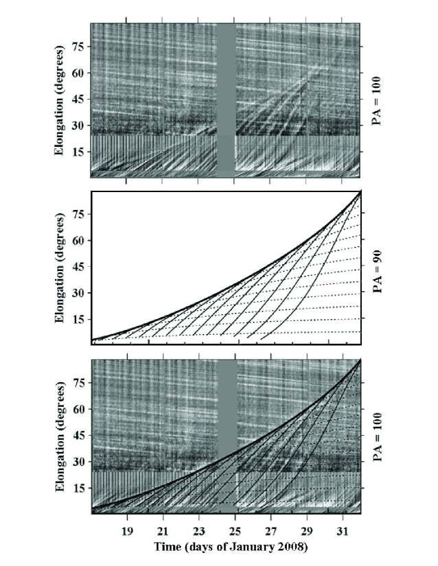
Figure 3: A comparison between the elongation/time tracks seen from STEREO-A during 2008 January 18–31 (top panel) and the calculated tracks from Fig. 2 with $\delta$ $\leq$ 60^∘ (middle panel). As seen in the superimposed images (bottom panel), the observed tracks and their envelope are well fit by the calculated curves.

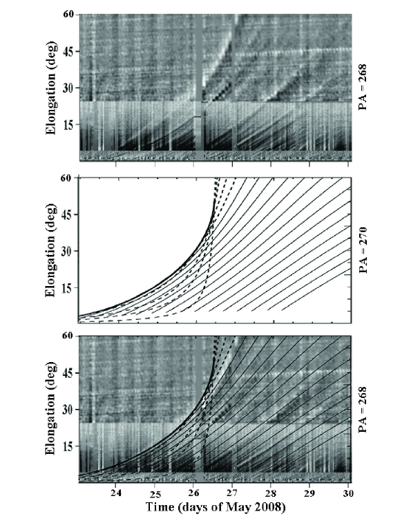
Figure 5: A comparison between the elongation/time tracks seen from STEREO-B during 2008 May 23–29 (top panel) and the calculated tracks from Fig. 4 (middle panel). As shown in the superimposed images (bottom panel), the observed tracks correspond to sky-plane elevations, $\delta$, in the range (75^∘, 15^∘).

Figure 3 compares an elongation/time map, obtained at a position angle of 100^∘ during 2008 January 17–31 (upper panel), with the calculated tracks from Figure 2 (middle panel). The STEREO-A elongation/time map consists of three sections merged together to span the COR2 ($0.5{{}^{\circ}}-4.0{{}^{\circ}}$), HI1 ($3.2{{}^{\circ}}-23.3{{}^{\circ}}$), and HI2 ($18.4{{}^{\circ}}-88.4{{}^{\circ}}$) fields of view. After transforming the offpointed HI1 and HI2 images into a Sun-centered polar coordinate system, radial strips at a particular position angle ($100{{}^{\circ}}$ in this case) are extracted and stacked chronologically to form a rectangular map of intensity difference as a function of time (horizontal axis) and elongation angle (vertical axis). These STEREO-A maps are crossed by a background of downward sloping tracks, which correspond to stars or the remnants of star images that escaped the differencing used to remove them from the HI2 images. As we will see later in Figure 5, the west-to-east motion of the stars produces upward slanting tracks in the STEREO-B elongation/time maps. Finally, in the top panel, the vertical bar on January 24 corresponds to a data gap. Additional details of the elongation/time maps and their construction are described elsewhere (Sheeley, 1999; Sheeley et al., 2007, 2008b; Rouillard et al., 2008, 2009; Davies et al., 2009).

In Figure 3, the tracks of interest are the ones of positive slope, which resemble the calculated tracks and correspond to the motions of streamer blobs moving outward from the Sun. In transferring the calculated maps from Figure 2 to the middle panel of Figure 3, we omitted tracks with values of $\delta$ equal to $70{{}^{\circ}},~{}80{{}^{\circ}}$, and $~{}89{{}^{\circ}}$ because tracks with $\delta$ greater than $60{{}^{\circ}}$ do not occur in the top panel of Figure 3. Such missing high-$\delta$ tracks are a characteristic of the STEREO-A observations, as we will discuss later.

The lower panel shows the result of superimposing the calculated tracks (middle panel) and the observed elongation/time map (upper panel). Not only do the calculations accurately reproduce the envelope, but they also reproduce most of the individual tracks. For a given value of Sun-spacecraft distance, $a$, the quality of the fit depends on the speed, $v_{r}$ ($330~{}km~{}s^{-1}$), and the Sun’s synodic angular rotation rate, ${\omega}$ ($0.233~{}rad~{}day^{-1}$). But it does not depend on the value of the assumed normalized radius, $\rho_{0}$, which disappeared when the calculated pattern was shifted in time to match the observed pattern. Allowing for a two-day section that was cropped from the start of the observed maps, the entire pattern extends for 17 days.

2.2 STEREO-B

Figure 4 shows a STEREO-B plot of elongation angle $\alpha$ versus time for values of $\delta$ ranging from 89^∘ to 0^∘, again calculated for a radial speed $v_{r}=330~{}km~{}s^{-1}$. The five tracks with $\delta~{}{\geq}~{}75{{}^{\circ}}$ graze the envelope twice at points that become increasingly closer together, and are plotted with dashed lines. The remaining tracks do not intersect the envelope and are plotted with narrow solid lines. Again, we plot the envelope with a thick solid line. Whereas the STEREO-A envelope lasted for about 18 days (corresponding to half the solar rotation time plus the Sun-A transit time), this STEREO-B envelope lasts only about 5 days corresponding to the Sun-B transit time ($a/v_{r}$).

Figure 5 compares an elongation/time map of COR2-B, HI1-B, and HI2-B images obtained at a position angle of 268^∘ during 2008 May 23-29 (upper panel), with the corresponding section of Figure 4 (middle panel). As before, their superposition is in the bottom panel. As we found previously (Sheeley et al., 2008a; Rouillard et al., 2008), this western view from STEREO-B is quite different from the eastern view from STEREO-A with most of the STEREO-B tracks spreading apart. This behavior is reproduced in the calculations. In this particular comparison, the observed tracks span a range of $\delta$ running from 15^∘ to 75^∘. In fact, the track of largest $\delta$ lies between the last dashed curve ($\delta$ = 75^∘) whose intersections with the envelope nearly coalesce and the first narrow solid curve ($\delta$ = 70^∘), which just misses the envelope.

2.3 The locus of enhanced visibility

We have defined the family of elongation/time tracks that results when ejections are released from a fixed point on the rotating Sun, and we have seen that these tracks have a common envelope. In Appendix 5.1, we deduce the equation of this envelope and show that it corresponds to the locus of points where the spiral of ejections is seen edge on. In a ($\rho$, $\delta$) polar coordinate system, this locus is described by a quadratic equation

$${\rho}^{2}-{\rho}~{}sin{\delta}~{}{\pm}~{}{\nu}~{}cos{\delta}~{}=0~{},$$ (4)

where ${\nu}~{}=~{}{v_{r}}/{\omega}a$; the minus sign applies to STEREO-A and the plus sign applies to STEREO-B.

It is easy to characterize the roots of this equation. For STEREO-A, there is only one positive, real root given by

$$\rho~{}=~{}\frac{sin{\delta}+\sqrt{sin^{2}{\delta}+4{\nu}~{}cos{\delta}}}{2}~{}.$$ (5)

For STEREO-B, the there are no positive, real roots unless $\delta$ exceeds a critical angle, ${\delta_{c}}$, given by

$$cos{\delta_{c}}~{}=~{}\sqrt{(2{\nu})^{2}+1}-2{\nu}~{}.$$ (6)

For a nominal solar wind speed of $330~{}km~{}s^{-1}$, $\nu\approx 0.8$, and $\delta_{c}$ is about 73^∘. Thus, in STEREO-B, blobs can pass in front of each other only if they originate far from the sky plane where $\delta~{}\geq~{}\delta_{c}$. In this case, there are two positive, real roots given by

$${\rho}~{}=~{}\frac{sin{\delta}{\pm}\sqrt{sin^{2}{\delta}-4{\nu}~{}cos{\delta}}}{2}~{}.$$ (7)

We have plotted these relations in Figure 6. For STEREO-A, the locus lies left of the Sun-spacecraft line in the region of negative X. For STEREO-B, the two ‘roots’ join continuously together in the region of positive X and combine with the STEREO-A locus to form a closed curve with a bean-like shape. (The link between STEREO-A and STEREO-B would not be continuous if we had used the slightly different radial distances of these two spacecraft from the Sun. But for an idealized observer that can look both east and west, the curve is continuous.)

Because the Thomson scattered intensity increases where the blobs line up, we have called this bean-shaped curve the ‘locus of enhanced visibility’. As we will see in the next section, this locus is useful for tracking streamer blobs through the STEREO fields of view, especially in combination with a knowledge of the location of the Thomson sphere (Vourlidas & Howard, 2006).

In Figure 6, we have represented the Thomson sphere ($\rho$ = sin$\delta$) by a dashed circle. Also, we have plotted Sun-centered spirals at intervals of 45^∘ as thin solid lines to simulate the corotating spiral of compressed blobs. In the region of negative X where STEREO-A observes, the locus of enhanced visibility lies outside the Thomson sphere, as expected from equation (5) where $\rho$ is always greater than sin$\delta$. However, in the region of positive X where STEREO-B observes, the locus lies inside the Thomson sphere as expected from equation (7) where both roots are less than sin$\delta$.

Equation (7) provides an even more stringent constraint on the locus as seen from STEREO-B. One value of $\rho$ is less than $sin{\delta}/2$ and the other value is greater than $sin{\delta}/2$. This means that these two positive roots correspond to segments of the STEREO-B curve that respectively lie inside and outside a small circle given by $\rho=sin{\delta}/2$. This circle is dotted in Figure 6. As shown in Appendix 5.2, this circle divides the sky into an inner region where background ejections appear to outrun foreground ejections against the sky, and an outer region where foreground ejections appear to outrun background ejections.

Thus, in STEREO-B, a radial ejection either does not intersect the locus of enhanced visibility at all, or it intersects the locus in two places. In the latter case, a blob would become aligned with other ejections twice on its way out from the Sun - first inside the dotted circle where ejections closer to the sky plane would appear to pass it, and again outside the circle where the blob would appear to overtake background ejections. However, this idealized behavior would happen for only a small range of sky-plane elevations, $\delta$, greater than about 73^∘; for real blobs with finite angular extents, we can regard the locus as being approximately radial most of the way outward from the Sun. Even ejections that miss the locus would still be closely confined between the locus and the Thomson sphere (provided that they lie on the front side of the Sun), and therefore frontside ejections would remain visible until they move beyond the Thomson sphere. By comparison, a streamer blob would encounter the locus of enhanced visibility only once in STEREO-A; this location would be outside the dotted circle where foreground ejections always pass background ejections along the line of sight.

With these new results, we are prepared to interpret STEREO observations of streamer blobs as they are compressed into a corotating spiral by fast wind from low-latitude coronal holes.

3 OBSERVATIONS

In the previous section, we showed that the STEREO elongation/time tracks of streamer blobs are consistent with a model of ejections moving radially outward from a fixed longitude on the rotating Sun. Also, we found that the envelopes of these tracks correspond to a bean-shaped locus where ejections pass in front of each other along the line of sight and their corotating spiral is seen edge on. In STEREO-A, the locus does not correspond to the track of any particular ejection, but is a wavefront where individual blobs surge forward to lead the cloud and then fade. In STEREO-B, the locus extends nearly radially outward from the Sun about 73^∘ from the sky plane, causing streamer blobs that are ejected in this direction to remain visible most of the way outward from the Sun. Next, we use observations from STEREO-A and STEREO-B to verify these conclusions.

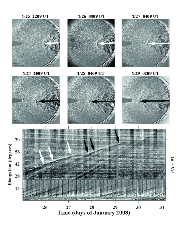
Figure 7: HI2-A images (top two rows) and a composite COR2-HI1-HI2 elongation/time map (bottom), showing the replacement of streamer blobs at the leading edge of the cloud. A compressed blob (white arrows) surges forward to take the lead before being overtaken along the line of sight by another blob (black arrows) located farther from the plane of the sky. The envelope of tracks marks the leading edge of the corotating spiral as seen from STEREO-A.

Figure 7 compares HI2-A images (top rows) with a corresponding elongation/time map obtained at a position angle of 91^∘. In the upper row, the white arrows indicate the outward motion of a compressed streamer blob at the leading edge of the cloud of ejections. The corresponding track is indicated by the white arrows in the bottom panel. The blob fades after 0409 UT on 2008 January 27 and gives up the lead to another blob indicated by black arrows in the second row. The track of this second blob is indicated by black arrows in the bottom panel. In this way, each blob surges forward to briefly take the lead and to make its brief contribution to the envelope of tracks. This wave of ‘billowing blobs’ marks the passage of the corotating spiral as it sweeps through the eastern hemisphere.

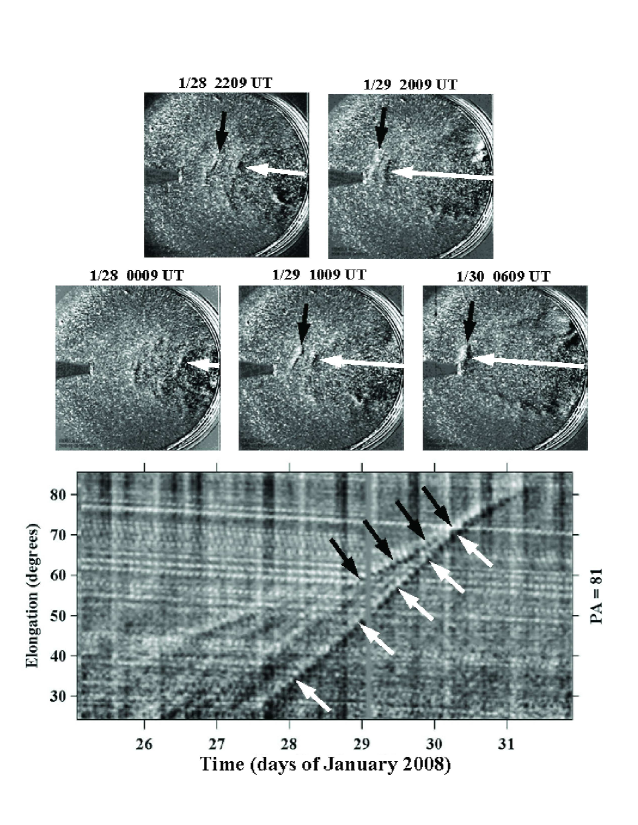
Figure 8: HI2-A images (alternating between the middle and top panels) and a HI2-A elongation/time map (bottom panel), showing the last visible ejection (white arrows) moving forward to take the lead from its most recent leader (black arrows). Similar replacements occur at adjacent position angles, producing the bow-shaped wave with the rippled fine structure seen in the last image at 0609 UT on January 30.

Figure 8 provides a similar comparison during 2008 January 28–30, as the last detectable streamer blob (shown by the white arrows) moves forward to take the lead from a prior blob (shown by black arrows). By 0609 UT on January 30, similar ejections at higher and lower latitudes have given the wave a large bow shape with small-scale ripples along its flanks. This is the curved wave that Wood et al. (2010) tracked back to a coronal streamer winding around the leading edge of a low-latitude coronal hole.

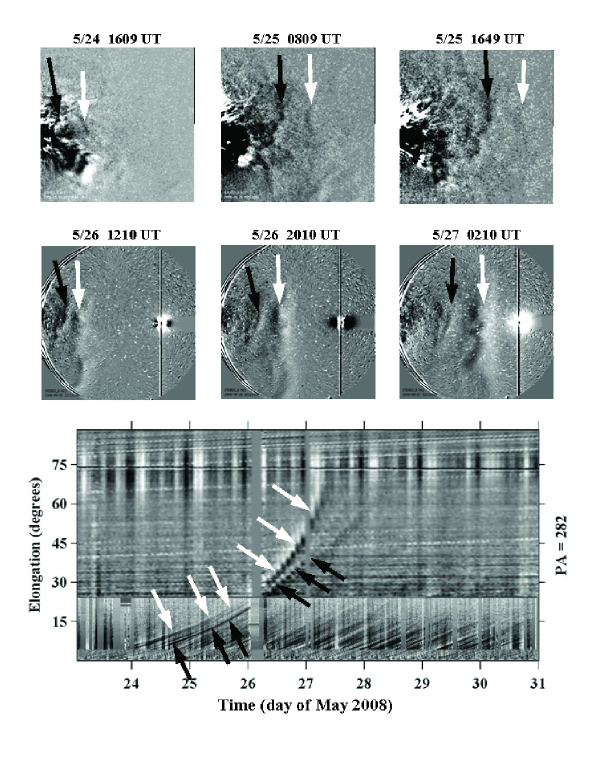
Figure 9: HI1-B images (top row), HI2-B images (middle row), and a composite COR2-HI1-HI2 elongation/time map (bottom panel), showing streamer blobs that were ejected close to the locus of enhanced visibility during 2008 May 23–30. The track with ${\delta}=73^{\circ}$ (white arrows) approaches the track with ${\delta}=60^{\circ}$ (black arrows) in the HI1 field of view and separates again in the HI2 field.

Figure 9 shows a similar comparison of STEREO-B observations. Here, the elongation/time tracks appear continuous from 1 AU all the way back to the lower corona. They correspond to single ejections rather than a wave of contributions as shown in the STEREO-A images. The first ejection (white arrows) was directed $73^{\circ}$ out of the sky plane and second ejection (black arrows) was directed $60^{\circ}$ out of the plane. Their tracks move toward each other in the HI1 field of view and away again in the HI2 field, just as we found in Figure 4 for tracks close to the critical angle. Apparently, these blobs remained closely aligned along our line of sight until they reached the middle of the HI2-B field of view. Like the HI2-A wave in Figure 8, these HI2-B waves in Figure 9 have a rippled fine structure, apparently reflecting the contributions of individual blobs.

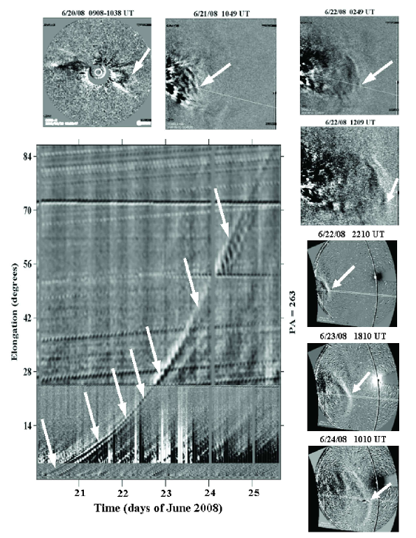
Figure 10: (clockwise from the upper left) A time sequence of images during 2008 June 20–24, showing the evolution of a face-on streamer blob (white arrow in the COR2-B image) as it becomes compressed into an azimuthal structure in the HI1-B field and sweeps past comet Boattini in the HI2-B field. (lower left) The corresponding elongation/time map, showing the complete track of motion with the instantaneous positions indicated by white arrows. In the last image, the radial lines have been shifted slightly northward from their true location so that they do not obscure the comet tail.

Figure 10 shows an ejection that can be followed continuously through the fields of COR2-B, HI-B, and HI2-B during 2008 June 20-25. It began as an unremarkable face-on blob, indicated by the arch-shaped feature in the upper left image. However, this initially unimpressive feature evolved into a pronounced azimuthal wave as it moved through the HI1-B field, where we suppose that it was compressed by the fast wind from the coronal hole behind it. The ejection is finally visible as a large, curved wave in the HI2-B field where it disrupted the tail of comet Boattini before sweeping past Earth. Because we are able to track this impressive feature continuously back to the Sun, we know that it did not begin in a dramatic event that somehow escaped our view. Rather, it gained its impressive stature gradually in the HI1-B field as material was swept up and compressed by the fast wind from the coronal hole.

As described previously (Sheeley et al., 2008a, b; Rouillard et al., 2008, 2009), we can fit the well-defined STEREO-B track with equations (2) and (3), corresponding to a radial trajectory at a constant speed from a location about 20$R_{\odot}$ from the Sun. In this case, we find that ${\delta}~{}{\approx}~{}64{{}^{\circ}}$ and $v_{r}~{}{\approx}~{}370~{}km~{}s^{-1}$. Thus, the elevation angle of this ejection was only $10{{}^{\circ}}$ less than the critical angle of $74{{}^{\circ}}$ needed for this $370~{}km~{}s^{-1}$ ejection to graze the STEREO-B envelope. This closeness to the envelope allowed us to detect the blob continuously from the Sun to 1 AU and to determine its origin as a face-on blob.

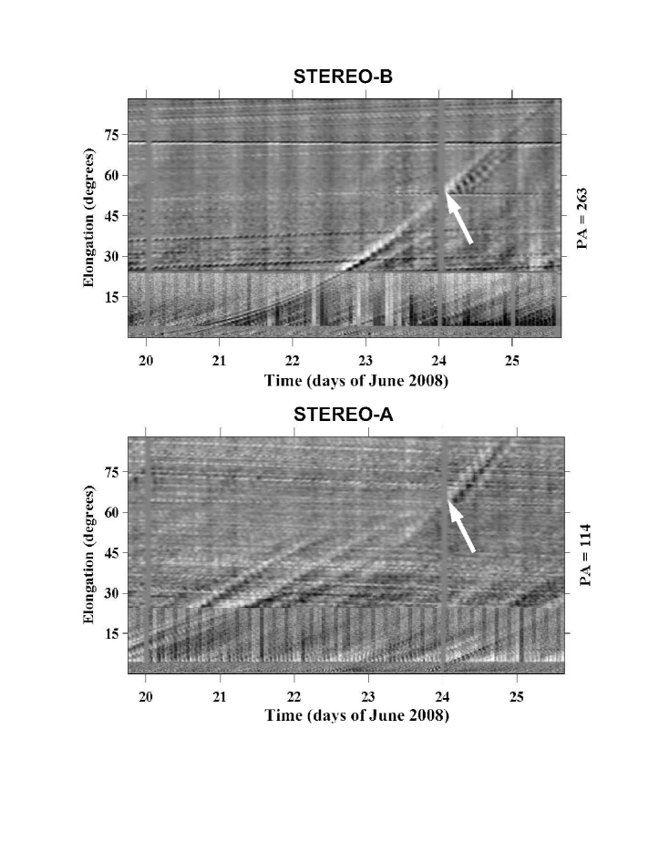
Figure 11: Comparison of STEREO-A and STEREO-B elongation/time maps during 2008 June 19–25 when the fast wind from a coronal hole swept up a streamer blob and disturbed the tail of comet Boattini (white arrows), which was located nearly midway between the two spacecraft on the Sun-Earth line. Despite the symmetry between the comet’s location in these two fields of view, only in STEREO-B can the wave be traced back to its origin in the lower corona.

Figure 11 compares this STEREO-B elongation/time map with the corresponding map obtained for STEREO-A. Because comet Boattini was located just south of the Sun-Earth line, approximately equidistant from STEREO-A and STEREO-B, its STEREO-A elongation angle should also be about ${\delta}=64{{}^{\circ}}$. But the corresponding track in STEREO-A is not visible in COR2-A or HI1-A, and it was hardly visible in HI2-A until the comet arrived on June 24. This is typical of streamer blobs ejected farther than about $60^{\circ}$ from the STEREO-A sky plane. Referring to Figure 6, we suppose that the reduced visibility of such streamer blobs is caused by their unfavorable locations far from the sky plane, well inside the Thomson sphere, and far from the locus of edge-on views. Figure 11 also illustrates that comets, as well as streamer ejections, can serve as tracers of CIRs.

4 SUMMARY AND DISCUSSION

Using a model in which streamer blobs are ejected from a fixed point on the rotating Sun, we derived an equation for their elongation/time tracks as seen from STEREO-A and STEREO-B. We showed that these two sets of tracks had envelopes similar to structures seen in the elongation/time maps of observed data. We derived equations for those envelopes and found that they described the places that streamer blobs pass each other along the line of sight. These are also the places that one observes the corotating spiral of compressed blobs edge on. We solved these equations and obtained a bean-shaped curve in the Sun’s equatorial plane. Because the Thomson scattered intensity is increased where blobs pass each other along the line of sight, we called this curve ‘the locus of increased visibility’. Like the Thomson sphere (Vourlidas & Howard, 2006; Thernisien, 2008), this locus provides a way of interpreting the visibility of streamer blobs as they pass through the STEREO fields of view.

Although this locus describes the places that the corotating spiral is seen edge on (i.e its leading edge), the locus itself is not a spiral. Rather it is a bean-shaped curve whose east-west asymmetry accounts for the differing visibility of blobs in STEREO-A and STEREO-B images. Prior to the launch of STEREO, it was generally supposed that solar ejections would fade out soon after passing the Thomson sphere (Vourlidas & Howard, 2006). In STEREO-A, the locus of enhanced visibility lies outside the Thomson sphere, creating a crescent-shaped region between these two boundaries where the ejections remain visible. However, for sky-plane elevations, $\delta$, greater than about $60^{\circ}$, streamer blobs are seldom visible because they are located far from the sky plane and well inside both the Thomson sphere and the locus of enhanced visibility for most of their trip outward from the Sun.

In the STEREO-B field of view the locus is oriented almost radially, and ejections close to this direction ($\delta{\approx}73^{\circ}$) remain continuously visible most of the way outward from the Sun. Even for lower values of $\delta$, the radial paths of frontside ejections lie close to the locus and to the Thomson sphere. Consequently, they remain visible until they pass the Thomson sphere. This explains why we are able to track streamer blobs continuously outward from the Sun in the STEREO-B images, but not in STEREO-A images.

In Figures 7–11, we used STEREO observations to illustrate these ideas. Figures 7 and 8 showed streamer blobs replacing each other at the leading edge of the cloud and contributing to the envelope of their elongation/time tracks. Now, we know that this ongoing replacement is a consequence of the motion of blobs past the locus of enhanced visibility where the corotating spiral is seen edge on. Figure 9 showed STEREO-B elongation/time tracks approaching each other close to the Sun and then separating again in the HI2-B field of view, as we now expect for streamer blobs that are ejected close to the nearly radial segment of the locus of enhanced visibility.

Figure 10 showed a large HI2-B wave that we tracked continuously back to a face-on streamer blob in the COR2-B field of view, and Figure 11 showed that we could not track the corresponding HI2-A wave back to its origin. It is easy to understand why we could not track the feature in STEREO-A; it was ejected $\sim$64^∘ from the STEREO-A sky plane and spent most of its time poorly visible inside the Thomson sphere. However, it is not easy to understand how such a large HI2 wave could be generated by compressing a single streamer blob. Perhaps this observation is reminding us that streamer blobs are just tracers of the more massive sweeping that occurs when fast wind runs into the streamer. This continuous flow would not be visible in our running difference images, but its compressed plasma might eventually be seen in the HI2 field of view, as Wood et al. (2010) supposed. In this sense, one could think of the streamer as being composed of many unresolved blobs. We also need to appreciate that the unambiguous association applies only at one position angle along the HI2 wave, and that neighboring parts of the wave front may be associated with other blobs.

The fast wind from the coronal hole is essential for tracking these ejections into the heliosphere. Discrete ejections occur everywhere along the streamer belt at the rate of about $4-6~{}day^{-1}$, (Sheeley et al., 1997; Wang et al., 1998), but if those ejections are not compressed by fast wind from a coronal hole, then their radial expansion will cause them to fade toward the end of the HI1 field of view. Consequently, the surviving blobs originate just ahead of the coronal hole where the streamer is distorted into a north-south segment and appears face on (Sheeley et al., 2008a; Rouillard et al., 2008, 2009, 2010; Wood et al., 2010).

The same argument applies to the continuous flow from a streamer, whose face-on segment is compressed into a corotating interaction region (CIR) (Gosling & Hundhausen, 1977; Burlaga, 1995). Tappin & Howard (2009) recently focused on the CIR, calculating its expected structure and looking for its observational signatures in the STEREO and the Solar Mass Ejection Imager (SMEI) fields of view. The centerpiece of their study was the ‘spine’ or ‘backbone’ that lies along the upper edge of the pattern of STEREO-A elongation/time tracks. They identified this feature with the leading edge of the CIR where the density spiral is seen edge on, and they regarded the more rapidly rising tracks to be ‘irregularities or waves’ ahead of the CIR. Likewise, they regarded the STEREO-B tracks to be signatures of ‘knots and waves’ that had not yet formed a stable leading edge.

It is instructive to consider why the blobs become more visible when they cross the bean-shaped locus and pass each other along the line of sight. As we mentioned in Section 2.3, the coalignment of two blobs would increase the Thomson scattered intensity simply by adding more scattering material along the line of sight. However, if the blobs themselves were compressed and squashed along the spiral, then their edge-on orientation would provide an even greater contribution than what would be obtained for randomly oriented blobs or uncompressed blobs passing each other along the line of sight. Images like those shown in Figures 7 and 10 give us the impression that the blobs are being compressed as they pass through the HI1 field of view, and it is tempting to suppose that the dominant effect comes from the alignment of their flat edges as the spiral is seen edge on.

In STEREO-A, the edge-on views occur for only a day or two because the radially moving blobs cross the bean-shaped locus nearly normal to its boundary. However, in STEREO-B, the coalignment lasts for almost the entire 5-day transit to 1 AU, until the blobs finally peel away from each other and reveal large waves in the HI2-B field of view.

In this paper, we limited our attention to streamer blobs being swept up by high-speed streams from low-latitude coronal holes, and we did not consider the streamer disconnection events (Wang et al., 1999; Simnett et al., 1997) and ‘streamer blowout’ coronal mass ejections (Howard et al., 1985; Sheeley et al., 2007; Sheeley & Wang, 2007), which we also expect to be swept up by the high-speed streams. As in previous studies, we were led to the idea that streamer blobs are tracers, but now with face-on blobs revealing the formation of CIRs in much the same way that edge-on blobs reveal the acceleration of the solar wind (Sheeley et al., 1997). It is only a short step further to suppose that the main portion of the solar wind originates in open magnetic field regions (whose coronal divergence determines the wind speed), and that everything else (blobs, streamer detachments, ‘streamer blowout’ CMEs, and the unresolved streamer itself) is just tracer material ejected into that wind.

5 APPENDIX

5.1 The Envelope Equation

In this section, we derive an equation for the envelope of the family of elongation/time tracks, and we show that it corresponds to the locus of places that the corotating spiral of streamer blobs is seen edge on. We begin by writing equation (2) in the form

$$tan{\alpha}~{}=~{}\frac{{\rho}(t,{\delta})~{}cos{\delta}}{1-{\rho}(t,{\delta})~{}sin{\delta}}~{},$$ (8)

where ${\rho}(t,{\delta})$ is given by equation (3). It is well known that the envelope of such a family of curves is obtained by combining this equation with its partial derivative with respect to $\delta$. Taking this derivative and keeping $\alpha$ and $t$ constant, we find that

$${\rho}^{2}-{\rho}~{}sin{\delta}+{\rho^{\prime}}~{}cos{\delta}~{}=0,$$ (9)

where ${\rho^{\prime}}=-({v_{r}}/a)~{}{t^{\prime}_{0}}({\delta})$. In this case, ${\rho^{\prime}}={\pm}{v_{r}}/{\omega}a$, with the minus sign for STEREO-A and the plus sign for STEREO-B. For convenience, we define ${\nu}={v_{r}}/{\omega}a$, and write ${\rho^{\prime}}={\pm}{\nu}$. Together these relations define the envelopes for STEREO-A and STEREO-B. In Section 5.3 of this appendix, we will provide an alternate definition in terms of the elongation angle, $\alpha$ and the normalized radial distance, $\rho$.

The same relations are obtained for the locus of points where the spiral of ejections is seen edge on. To see this, we return to Figure 1 and look along the line that extends from point A through point P and beyond. Our objective is to keep the elongation angle, $\alpha$, constant and ask how the normalized radial distance, $\rho$ changes as the elevation angle, $\delta$, is varied. For this purpose, we simply take the derivative of equation (8) with respect to $\delta$ while keeping $\alpha$ constant. The result is again given by equation (9). So if $\rho$ changes with $\delta$ as given by this equation, then neighboring ejections will lie along our line of sight from point A to point P and beyond. For these ejections to also lie on the spiral, the rate of change, ${\rho^{\prime}}$, must be obtained from equation (3), in which case ${\rho^{\prime}}={\pm}{\nu}$ with the minus sign for STEREO-A and the plus sign for STEREO-B. Thus, the locus of edge-on views and the envelope of tracks are determined by the same equations and therefore are the same.

5.2 Separating the angular speeds of foreground and background ejections

The dotted circle in Figure 6 divides the heliosphere into an inner region where background ejections outrun foreground ejections against the sky, and an outer region where foreground ejections outrun background ejections. To see this, we first hold $\delta$ constant and calculate the angular rotation rate $\dot{\alpha}$. Then, we hold $\alpha$ constant and determine how $\dot{\alpha}$ changes with $\delta$. We expect to find that ${\partial}{\dot{\alpha}}/{\partial}{\delta}$ is positive outside the dotted circle and negative inside it. We begin with equation (1). Taking the time derivative and recognizing that $\dot{\rho}$ = $v_{r}/a$, we find that

$$\dot{\alpha}~{}=~{}{\frac{v_{r}}{a}}~{}\frac{cos^{2}(\alpha-\delta)}{cos{\delta}}$$ (10)

Thus, for a given direction, $\delta$, a blob reaches its largest angular speed, $\dot{\alpha}$, at the Thomson sphere where ${\alpha}={\delta}$ and the intensity is greatest.

Next, we hold $\alpha$ constant, and take the logarithmic derivative of equation (10) with respect to $\delta$. Combining the result with equation (2), we obtain

$$\frac{1}{\dot{\alpha}}\frac{{\partial}{\dot{\alpha}}}{{\partial}{\delta}}~{}=~{}\frac{2\rho-sin\delta}{cos\delta}$$ (11)

and therefore

$$\frac{{\partial}{\dot{\alpha}}}{{\partial}{\delta}}~{}=~{}{\frac{v_{r}}{a}}~{}\frac{cos^{2}(\alpha-\delta)}{cos^{2}\delta}~{}(2\rho-sin\delta).$$ (12)

From this equation, it is clear that the angular rotation speed $\dot{\alpha}$ increases with $\delta$ outside the circle (where $\rho=sin{\delta}/2$), shown dotted in Figure 6, and decreases with $\delta$ inside that circle. This means that background ejections appear to overtake foreground ejections inside the dotted circle and foreground ejections appear to overtake background ejections outside the circle.

5.3 Elongation angles along the locus of enhanced visibility

In Section 5.1, we wrote the envelope equation as a relation between normalized radial distance, $\rho$, and the ejection’s elevation angle, $\delta$, out of the sky plane. Now, we wish to rewrite this equation as a relation between the elongation angle, $\alpha$, and the normalized radial distance, $\rho$. We could obtain the desired relation by simply eliminating $\delta$ from equations (2) and (4). However, it is instructive, and perhaps easier, to take a physical approach. In this case, we recognize that for a spiral

$$tan({\alpha}-{\delta})~{}=~{}\frac{{\partial}{\rho}}{{\rho}~{}{\partial}{\delta}}~{}=~{}\frac{v_{r}}{{\omega}{r}}~{}=~{}\frac{\nu}{\rho}~{}.$$ (13)

Solving this equation for $cos({\alpha}-{\delta})$ and then equating it to the value of $cos({\alpha}-{\delta})$ given by equation (1), we obtain the desired result:

$$sin{\alpha}~{}=~{}\frac{{\rho}^{2}}{\sqrt{{\nu}^{2}+{\rho}^{2}}}~{}.$$ (14)

This equation is useful for identifying a point along the envelope in an elongation/time map if the value of $\rho$ is known or easily calculated. For example, if we wish to identify the point in Figure 4 where the two STEREO-B tangents coalesce, we set ${\delta}={\delta_{c}}$ in equation (7) and obtain ${\rho}=sin{\delta_{c}}/2$. Then, using ${\nu}~{}{\approx}~{}0.8$ in equations (6) and (14), we find that ${\alpha}~{}{\approx}~{}14.2{{}^{\circ}}$, consistent with a location midway between the tangent points of the dashed curves in Figure 4.

The STEREO/SECCHI data are produced by a consortium of NRL (US), LMSAL (US), NASA/GSFC (US), RAL (UK), UBHAM (UK), MPS (Germany), CSL (Belgium), IOTA (France), and IAS (France). In the US, funding was provided by NASA, in the UK by PPARC, in Germany by DLR, in Belgium by the Science Policy Office, and in France by CNES and CNRS. NRL received support from the USAF Space Test Program and ONR. We are grateful to our many colleagues in these organizations who made these observations possible. In particular, we would like to acknowledge Nathan Rich (NRL) and Tom Cooper (Cornell University) for a wide variety of programming assistance and Yi-Ming Wang (NRL) for his continued scientific help and advice. We have also benefited from helpful scientific discussions with Arnaud Thernisien (USRA) and Brian Wood (NRL).

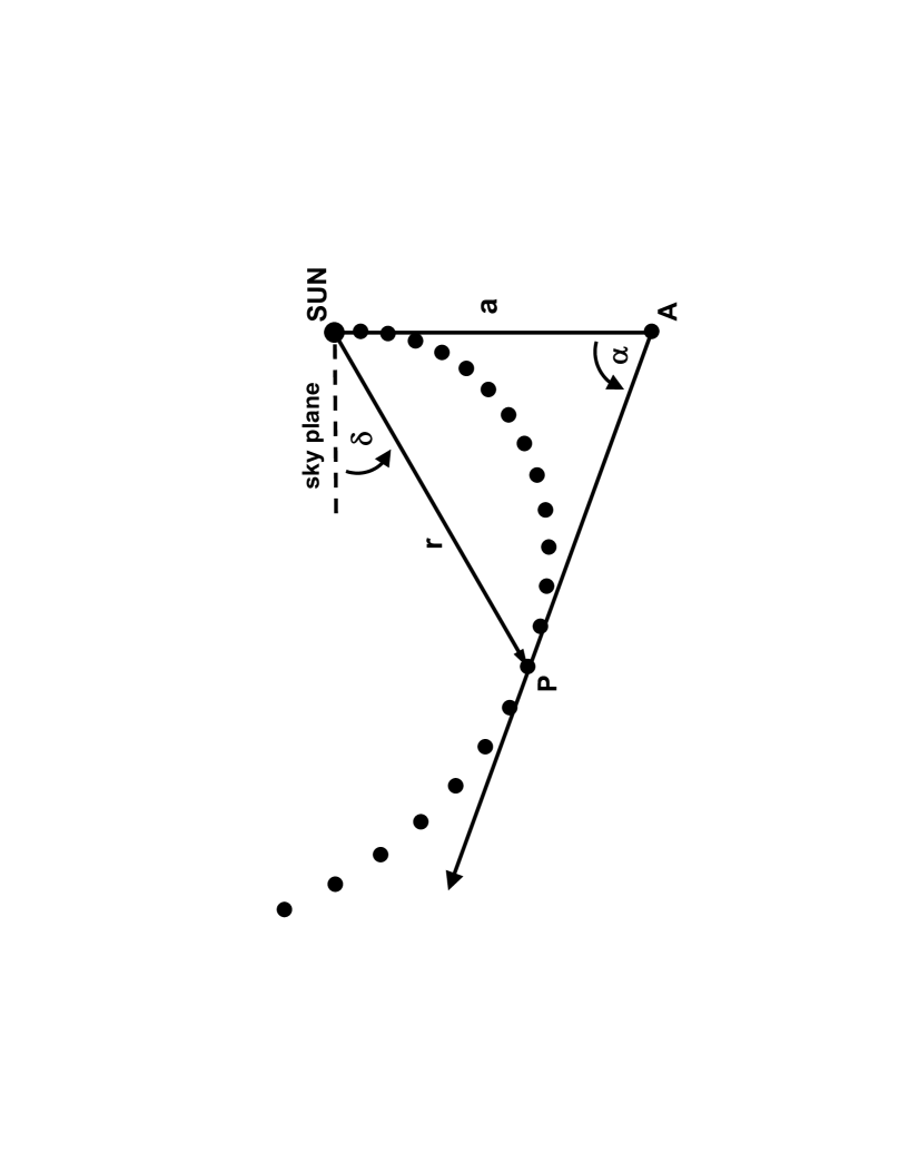
Figure 1: Sketch, illustrating the geometry of a family of streamer blobs moving radially outward from a fixed point on the rotating Sun. Looking $\alpha$ radians east of the Sun, the observer at point A sees the resulting spiral of ejections edge-on at the point P.

Figure 2: The eastern view. Tracks of elongation angle, $\alpha$, versus time, calculated for sky-plane elevation angles, $\delta$ = $-89{{}^{\circ}}$, -80^∘, -70^∘, -60^∘, …, 70^∘, 80^∘, 89^∘. Each ejection originates from a fixed longitude on a 27-day rotating sphere of radius $r_{s}$ = 20$R_{\odot}$ beyond which the radial speed, $v_{r}$, has a constant value of 330 km s^-1. Each track is plotted with a thin solid line until it reaches the common envelope, and then with a dotted line to emphasize the decreased visibility of the corresponding solar ejection.

Figure 4: The western view. Similar to Fig. 2 except that tracks are plotted for sky-plane elevation angles, ${\delta}$ = $89{{}^{\circ}}$, $87{{}^{\circ}}$, $85{{}^{\circ}}$, $80{{}^{\circ}}$, $75{{}^{\circ}}$, $70{{}^{\circ}}$, …, $10{{}^{\circ}}$, $5{{}^{\circ}}$, $0{{}^{\circ}}$. The five tracks with $\delta$ greater than the critical value, $\delta_{c}$ $\sim$ 73^∘, graze the envelope twice and are plotted with dashed lines; tracks with smaller values of $\delta$ miss the envelope and are plotted with solid lines.

Figure 6: A polar coordinate view of the Sun’s equatorial plane, showing the locus of enhanced visibility (thick solid curve) and the Thomson sphere (dashed circle). The Sun is at the origin, surrounded by a 20$R_{\odot}$ region of acceleration, and the observer is at the point (0, -1). Spirals of radially moving material are drawn at 45^∘ intervals. The observer sees the leading edge of the spiral moving along the bean-shaped locus. The dotted circle separates an inner region, where background ejections pass foreground ejections against the sky, from an outer region, where foreground ejections pass background ejections.

References

- Burlaga (1995) Burlaga, L. F. 1995, Interplanetary magnetohydrodynamics, by L. F. Burlaga, International Series in Astronomy and Astrophysics, Vol. 3, Oxford University Press. 1995. 272 pages; ISBN13: 978-0-19-508472-6, 3
- Davies et al. (2009) Davies, J. A., et al. 2009, Geophys. Res. Lett., 36, 2102
- Gosling & Hundhausen (1977) Gosling, J. T., & Hundhausen, A. J. 1977, Scientific American, 236, 36
- Howard et al. (2008) Howard, R. A., et al. 2008, Space Science Reviews, 136, 67
- Howard et al. (1985) Howard, R. A., Sheeley, N. R., Michels, D. J., & Koomen, M. J. 1985, J. Geophys. Res., 90, 8173
- Rouillard et al. (2008) Rouillard, A. P., et al. 2008, Geophys. Res. Lett., 35, 10110
- Rouillard et al. (2010) Rouillard, A. P., et al. 2010, J. Geophys. Res.
- Rouillard et al. (2009) Rouillard, A. P., et al. 2009, Sol. Phys., 256, 307
- Sheeley et al. (2009) Sheeley, N. R., Lee, D., Casto, K. P., Wang, Y., & Rich, N. B. 2009, ApJ, 694, 1471
- Sheeley (1999) Sheeley, N. R., Jr. 1999, in American Institute of Physics Conference Series, Vol. 471, American Institute of Physics Conference Series, ed. S. R. Habbal, R. Esser, J. V. Hollweg, & P. A. Isenberg, 41
- Sheeley et al. (2008a) Sheeley, N. R., Jr., et al. 2008a, ApJ, 674, L109
- Sheeley et al. (2008b) Sheeley, N. R., Jr., et al. 2008b, ApJ, 675, 853
- Sheeley & Wang (2007) Sheeley, N. R., Jr., & Wang, Y.-M. 2007, ApJ, 655, 1142
- Sheeley et al. (1997) Sheeley, N. R., Jr., et al. 1997, ApJ, 484, 472
- Sheeley et al. (2007) Sheeley, N. R., Jr., Warren, H. P., & Wang, Y.-M. 2007, ApJ, 671, 926
- Simnett et al. (1997) Simnett, G. M., et al. 1997, Sol. Phys., 175, 685
- Tappin & Howard (2009) Tappin, S. J., & Howard, T. A. 2009, ApJ, 702, 862
- Thernisien (2008) Thernisien, A. 2008, Ph.D. thesis, Université Paul Cézanne - Aix-Marseille III
- Vourlidas & Howard (2006) Vourlidas, A., & Howard, R. A. 2006, ApJ, 642, 1216
- Wang et al. (1999) Wang, Y.-M., Sheeley, N. R., Howard, R. A., Rich, N. B., & Lamy, P. L. 1999, Geophys. Res. Lett., 26, 1349
- Wang et al. (1998) Wang, Y.-M., et al. 1998, ApJ, 498, L165
- Wood et al. (2010) Wood, B. E., Howard, R. A., Thernisien, A., & Socker, D. G. 2010, ApJ, 708, L89