Automatic Probabilistic Program Verification through Random Variable Abstraction

Abstract

The weakest pre-expectation calculus [21] has been proved to be a mature theory to analyze quantitative properties of probabilistic and nondeterministic programs. We present an automatic method for proving quantitative linear properties on any denumerable state space using iterative backwards fixed point calculation in the general framework of abstract interpretation. In order to accomplish this task we present the technique of random variable abstraction (RVA) and we also postulate a sufficient condition to achieve exact fixed point computation in the abstract domain. The feasibility of our approach is shown with two examples, one obtaining the expected running time of a probabilistic program, and the other the expected gain of a gambling strategy.

Our method works on general guarded probabilistic and nondeterministic transition systems instead of plain pGCL programs, allowing us to easily model a wide range of systems including distributed ones and unstructured programs. We present the operational and $\mathit{wp}$ semantics for this programs and prove its equivalence.

1 Introduction

Automatic probabilistic program verification has been a field of active research in the last two decades. The two major approaches to tackle this problem have been model checking [23, 10, 3, 12], and theorem proving [13, 4]. Traditionally model checking has been targeted to be a push-button technique, but in the quest of full automation some restrictions apply. The most prominent one is finiteness of the state space, that leads to finite-state Markov chains (MC) and Markov decision processes (MDP). These models are usually verified against probabilistic extensions of temporal logics such as PCTL [10, 3]. Even with the finiteness restriction, the state explosion problem have to be alleviated using, for example, partial order reduction techniques [2]. Another approach is taken in the PASS tool [24, 11], where the authors profit from the work on predicate abstraction [9, 5] in the general framework of abstract interpretation [6] in order to aggregate states conveniently and prevent the state explosion problem or even handle infinite state spaces. Theorem proving techniques can also overcome state explosion and infinite state space problems but at a cost, the automation is up-to loop invariants, that is, once the correct loop invariants are fixed, the theorem prover can automatically prove the desired property [13]. There are also mixed approaches like [18] in the realm of refinement checking of pGCL programs.

Automatic probabilistic program verification cannot, to the author’s knowledge, tackle the problem of performance measurement of possibly unbounded program variables. Typical examples of this quantitative measurements are expected number of rounds of a probabilistic algorithm, or the expected revenue of a gambling strategy. In this kind of problems, the model checking approach discretize the variable up to a bound, either statically or using counterexample-guided abstraction refinement (CEGAR) [11], but since the values it can reach are unbounded, an approximation is needed at some point. In theorem proving this problem could be solved but the invariants have to devised, and anyone involved in this task knows that this is far from trivial.

We propose the computation of parametric linear invariants on a set of predefined predicates, and we call this random variable abstraction (RVA) as it generalizes predicate abstraction (PA) to a quantitative logic based on expectations [21]. Our motivation is simple. If the underlying invariants of the program can be captured as a sum of linear random variables in disjoint regions of the state space, a suitable fixed point computation should be able to discover the coefficients of such a linear expressions. To compute the coefficients we depart from the traditional forward semantics approach, and use weakest pre-expectation ($\mathit{wp}$) backwards semantics [21]. This combination of predicate abstraction, linear random variables and quantitative $\mathit{wp}$, renders a new technique that can compute, for example, expected running time of probabilistic algorithms, even though this quantities are not a-priori bound by any constant. This allows us to reason about efficiency of algorithms.

Parametric linear invariants for probabilistic and nondeterministic programs using expectation logic are also generated in [15], but our work differs in two aspects. First, in [15] all random variables have to be one-bounded or equivalently they should be bounded by a constant. Second, in the computation technique for the coefficients, they cast the problem to one of constraint-solving and resort to off-the-shelf constraint solvers, while we use a fixed point computation.

Outline. In Section 2 we first give a motivating example that briefly shows the type of problems we address as well as the mechanics to obtain the result. Then in Section 3 the probabilistic and nondeterministic programs, its operational and $\mathit{wp}$ semantics are presented, as well as the fixed point computation in the concrete domain of (general) random variables. Section 4 covers the abstract domain of random variables, its semantics, and the fixed point computation, as well as the general problems to face in this process. A more involved example is given in Section 5. Section 6 concludes the paper and discusses future work.

2 Motivating Example

In order to give some intuition on what we are going to develop throughout the paper, we present a purely probabilistic program $P_{0}$ that generates a geometric distribution.

$P_{0}$ $\triangleq$		$x,i:=1,0$
	;	do	$x\neq 0\rightarrow$
				$x:=0\oplus_{\frac{1}{2}}x:=1$
			;	$i:=i+1$
		od

Figure 1: Geometric distribution.

This program halts with probability 1 and variable $i$ could reach any natural number with positive probability. The semantics of this program can be regarded as a probability measure $\Delta$ over the naturals with distribution $\Delta.\{K<i\}=\tfrac{1}{2^{K}}$. The expected running time of the algorithm is precisely the expectation of random variable $i$ with respect to the measure $\Delta$, that is $\int_{\Delta}i$. Informally we could do this quantitative analysis as follows: the first iteration is certain, however the second one occurs with probability one half, the third one will occur with half the probability of previous one, and so on. In [21, p.69] the same calculation is done by hand, using the invariant $(i+K)\textit{\ if\ }(x\neq 0)\textit{\ else\ }i$, the equations fix $K=2$ and this implies that given the initialization, the expected value of random variable $i$ is $2$.

Our approach establishes a recursive higher-order function $f$ on the domain of random variables using weakest pre-expectation semantics [21]. It computes the expectation of taking a loop cycle and repeating, or ending.

$$f.X\triangleq[x\neq 0]\times\mathit{wp}.(x:=0\oplus_{\frac{1}{2}}x:=1;i:=i+1).X+[x=0]\times i$$

We are looking for a fixed point of this functional, namely $f.\varphi=\varphi$, but taking a specific subset of random variables: two linear functions on the post-expectation $i$, one for each region defined by the predicates that control the flow of the program. It is a parametric random variable with coefficients $((a_{1},a_{0}),(b_{1},b_{0}))$.

$$\textit{Inv}\triangleq(a_{1}i+a_{0})[x=0]+(b_{1}i+b_{0})[x\neq 0]$$

Calculating $f$ in the random variable Inv:

$$f.\textit{Inv}=(1i+0)[x=0]+(\tfrac{a_{1}+b_{1}}{2}i+\tfrac{a_{0}+a_{1}+b_{0}+b_{1}}{2})[x\neq 0]\enspace.$$

If we only look at the coefficients, $f$ can be (exactly) captured by function $f^{\sharp}$ on the domain $\mathbb{R}^{(1+1)\times 2}$.

$$f^{\sharp}.((a_{1},a_{0}),(b_{1},b_{0}))=((1,0),(\tfrac{a_{1}+b_{1}}{2},\tfrac{a_{0}+a_{1}+b_{0}+b_{1}}{2}))\enspace.$$

The computation goes as follows, from the random variable that is constantly $0$ represented by the tuple $((0,0),(0,0))$ we apply the update rule iteratively until the floating point precision produces a fixed point after a little less than half hundred iterations (Table 1).

	Coefficients
Iter.	($a_{1}$, $a_{0}$)	($b_{1}$, $b_{0}$)
0	(0, 0)	(0, 0)
1	(1, 0)	(0, 0)
2	(1, 0)	(0.5, 0.5)
3	(1, 0)	(0.75, 1)
4	(1, 0)	(0.875, 1.375)
5	(1, 0)	(0.9375, 1.625)
6	(1, 0)	(0.96875, 1.78125)
7	(1, 0)	(0.984375, 1.875)
⋮	⋮	(1,⋮
45	(1 ,0)	(1, 2)

Table 1: Iteration for the geometric distribution program.

These fixed point coefficients represent the random variable $i\times[x=0]+(i+2)\times[x\neq 0]$ that is a valid pre-expectation of the repeating construct with respect to post-expectation $i$. If we take the weakest pre-expectation of initialization (syntactic substitution) we obtain the value $2$. Note that invariant and expectation of random variable $i$ coincide with the calculations done by hand in [21].

3 Concrete Semantics

3.1 Probabilistic Programs

We fix a finite set of variables $X$. A state is a function from variables to the semantic domain $s:X\rightarrow\Omega$, and the set of all states is denoted by $S$. An expression is a function from states to the semantic domain $\beta:S\rightarrow\Omega$, while a boolean expression is a function $G:S\rightarrow\{\textsf{true},\textsf{false}\}$, and an assignment $E:S\rightarrow S$ is a state transformer. We define substitution of expression $\beta$ with assignment $E$, $\beta\langle E\rangle$ as function composition $\beta\circ E$.

A guarded command $(G\rightarrow E_{1}@p_{1}|\cdots|E_{k}@p_{k})$ consists of a boolean guard $G$ and assignments $E_{1},\cdots,E_{k}$ weighted with probabilities $p_{1},\cdots,p_{k}$ where $\sum_{i=1}^{k}p_{i}\leq 1$.

A program $P=(S,\mbox{\small$\mathcal{I}$},C)$ consists of a boolean expression $\mathcal{I}$ that defines the set of initial states and a finite set of guarded commands $C$.

Note that using this guarded commands we can underspecify (in the sense of refinement) in two ways. One way is using guard overlapping, so in the non-null intersection of $G_{0}$ and $G_{1}$ there is a nondeterministic choice between the two multi-way probabilistic assignments. The other is using subprobability distributions, since the expression $(E_{0}@\tfrac{1}{4}|E_{1}@\tfrac{1}{4})$ can be regarded as all the probability distributions that assign at least $\tfrac{1}{4}$ to each branch [8]. Later, in the operational model, we will see that the first one is handled by convex combination closure, while the later is handled by up closure.

3.2 Operational model

We fix the semantic domain $\Omega$ as a denumerable set, for example the rationals. The power set is denoted by $\mathit{\mathbb{P}}$, and if the empty set is not included we denote it $\mathit{\mathbb{P}^{+}}$.

The set of (discrete) sub-probability measures over $S$ is $\overline{S}=\{\Delta:S\rightarrow[0..1]\mid\sum\Delta\leq 1\}$. The partial order $\Delta\sqsubseteq\Delta^{\prime}$ on $\overline{S}$ is defined pointwise, and $\underline{0}$ denotes the least element everywhere defined $0$. A set of sub-probability measures $\xi\subseteq\overline{S}$ is up-closed if $\Delta\in\xi$ and $\Delta\sqsubseteq\Delta^{\prime}$ then $\Delta^{\prime}\in\xi$. Similarly $\xi$ is convex closed if for all $p\in[0..1]$ and $\Delta_{0},\Delta_{1}\in\xi$ implies $p\Delta_{0}+(1-p)\Delta_{1}\in\xi$. Finally $\xi$ is Cauchy-closed or simply closed if it contains its boundary, that is for every sequence $\{\Delta_{i}\}\subseteq\xi$, such that $\Delta_{i}\stackrel{{\scriptstyle i\rightarrow\infty}}{{\longrightarrow}}\Delta$, then $\Delta\in\xi$. $\mathit{\mathbb{C}S}$ is the set of non-empty, up-closed, convex and Cauchy-closed subsets of $\overline{S}$. The set of probabilistic programs over $S$ is defined $\mathit{\mathbb{H}S}\triangleq S\rightarrow\mathit{\mathbb{C}S}$, and it is ordered pointwise with ${}\sqsubseteq{}$.

The probabilistic and nondeterministic transition system $\mathcal{M}$ is a tuple $(S,\mbox{\small$\mathcal{I}$},\mbox{\small$\mathcal{T}$}\!)$ where $S$ is the set of states, $\mbox{\small$\mathcal{I}$}\subseteq S$ is a set of initial states, and an $\mbox{\small$\mathcal{T}$}\!\in\mathit{\mathbb{H}S}$ is called transition function.

The semantics of a program $P=(S,\mbox{\small$\mathcal{I}$},C)$ is the tuple $\mathcal{M}=(S,\mbox{\small$\mathcal{I}$},\mbox{\small$\mathcal{T}$}\!)$ with the same state space and initial states, where $\mbox{\small$\mathcal{T}$}\!.s$ is defined by its generators.

Definition 3.1.

Given the program $P=(S,\mbox{\small$\mathcal{I}$},C)$, where $C=\{i:[0..l)\mbox{\raisebox{1.72218pt}{\tiny$\>\;\bullet\;\>$}}(G_{i}\rightarrow E^{i}_{1}@p^{i}_{1}|\cdots|E^{i}_{k_{i}}@p^{i}_{k_{i}})\}$, the set of generators of $\mbox{\small$\mathcal{T}$}\!.s$ is $\mathbb{G}\mbox{\small$\mathcal{T}$}\!.s\triangleq\{i:[0..l)\mid G_{i}.s\mbox{\raisebox{1.72218pt}{\tiny$\>\;\bullet\;\>$}}\Delta_{i}\}$ if $(\exists i:[0..l)\mbox{\raisebox{1.72218pt}{\tiny$\>\;\bullet\;\>$}}G_{i}.s)$, otherwise $\mathbb{G}\mbox{\small$\mathcal{T}$}\!.s=\{\underline{0}\}$, where $\Delta_{i}.s^{\prime}=(\sum j:[1..k_{i}]\mid E_{j}^{i}.s=s^{\prime}\mbox{\raisebox{1.72218pt}{\tiny$\>\;\bullet\;\>$}}p_{j}^{i})$ .

The set $\mathbb{G}\mbox{\small$\mathcal{T}$}\!.s$ is nonempty and closed. Now $\mbox{\small$\mathcal{T}$}\!.s$ can be defined from above as the minimum set over $\mathit{\mathbb{C}S}$ that includes $\mathbb{G}\mbox{\small$\mathcal{T}$}\!.s$. Note this set is well defined since $\mathbb{G}\mbox{\small$\mathcal{T}$}\!.s\subseteq\overline{S}\in\mathit{\mathbb{C}S}$, and $\mathit{\mathbb{C}S}$ is closed by arbitrary intersections. We can also define $\mbox{\small$\mathcal{T}$}\!.s$ from below, taking the up and convex closure of the generator set $\mathbb{G}\mbox{\small$\mathcal{T}$}\!.s$. There is no need to take the Cauchy closure since the generator set is closed and the operators that form the up and convex closure preserve this property.

3.3 Expectation-transformer semantics

In the previous section a probabilistic and nondeterministic program semantics was defined as a transition function from states to a subset of subprobability distributions. This set was defined to be up and convex closed.

Verification of this particular type of programs poses the question of what propositions are in this context. We take the approach by Kozen [16], where propositions $Q:S\rightarrow\{\textsf{true},\textsf{false}\}$ are generalized as random variables, that is a measurable function $\beta:S\rightarrow\mathbb{R}_{\geq}$ from states to positive reals. The program $P$ is taken as a distribution function $\Delta$, and the program verification problem, formerly a boolean value $P\models Q$ is cast into an integral $\int_{\Delta}\beta$ that is the expectation of random variable $\beta$ given distribution $\Delta$. In a nutshell this is a quantitative logic based on expectations. Boolean operators are (no uniquely) generalized. The arithmetic counterpart of the implication is $\alpha\Rrightarrow\beta$, that is pointwise inequality $(\forall s:S\mbox{\raisebox{1.72218pt}{\tiny$\>\;\bullet\;\>$}}\alpha.s\leq\beta.s)$. Conjunction ${}\land{}$ can be taken as multiplication $\times$ or minimum ${}\sqcap{}$, and disjunction $\lor$ over non overlapping predicates is captured by addition ${}+{}$. The characteristic function operator $[\cdot]$ goes from the boolean to the arithmetic domain with the usual interpretation $[\textsf{true}]=1$, $[\textsf{false}]=0$, and using it we could define negation as subtracting the truth value from one $[\neg Q]=1-[Q]$.

This model generalizes the deterministic one since it is proven that $[P\models Q]=\int_{P}[Q]$ for predicate $Q$ and deterministic program $P$.

In [14] He et al. extend Kozen’s work to deal with nondeterminism as well as probabilism in the programs. The program verification problem is again a real value, namely the least expected value of the random variable with respect to the sub-probability distributions generated by the program (demonic nondeterminism).

Probabilistic (and nondeterministic) program verification problem is usually defined in the program text itself as Hoare triple semantics or the equivalent weakest precondition calculus of Dijkstra [16, 21]. The triple $\{Q\}P\{Q^{\prime}\}\equiv Q\Rightarrow\mathit{wp}.P.Q^{\prime}$ is generalized to $\{\alpha\}P\{\beta\}\equiv\alpha\Rrightarrow\mathit{wp}.P.\beta$, and the generalized $\mathit{wp}$ is called weakest pre-expectation calculus or probabilistic $\mathit{wp}$ semantics.

In general, the program outcome depends on the input state $s$, therefore $\mathit{wp}.P.\beta$ is a function that given the initial state establish a lower bound on the expectation of random variable $\beta$ (it is exact in the case of a purely probabilistic program). Therefore, expectations as functions of the input are also random variables, hence we define the expectation space as $\mathit{\mathbb{E}S}\triangleq\langle S\rightarrow\mathbb{R}_{\geq},\Rrightarrow\rangle$. It is worth noticing that all functions in $\mathit{\mathbb{E}S}$ are measurable since $S$ is taken to be denumerable (all subsets of $S$ are measurable). This implies that is valid to write integrals like $\int_{\Delta}f$ with $\Delta\in\overline{S}$ and $f\in\mathit{\mathbb{E}S}$. We define the expectation transformer space as the functions from expectations to expectations $\mathit{\mathbb{T}S}\triangleq\langle\mathit{\mathbb{E}S}\leftarrow\mathit{\mathbb{E}S},\sqsubseteq\rangle$.

The $\mathit{wp}$ expectation calculus is defined structurally in the constructors of probabilistic and nondeterministic programs (Fig. 2). This function basically maps assignments to substitutions, choice and probabilistic choice to convex combination and nondeterministic choice to minimum.

$$\mathit{wp}.\textbf{abort}.\beta \triangleq\underline{0}$$

$$\mathit{wp}.\textbf{skip}.\beta \triangleq\beta$$

$$\mathit{wp}.E.\beta \triangleq\beta\langle E\rangle$$

$$\mathit{wp}.(P_{0};P_{1}).\beta \triangleq\mathit{wp}.P_{0}.(\mathit{wp}.P_{1}.\beta)$$

$$\mathit{wp}.(P_{0}\oplus_{p}P_{1}).\beta \triangleq p\times\mathit{wp}.P_{0}.\beta+(1-p)\times\mathit{wp}.P_{1}.\beta$$

$$\mathit{wp}.(\textbf{if}\ G\ \textbf{then}\ P_{0}\ \textbf{else}\ P_{1}\ \textbf{fi}).\beta \triangleq\mathit{wp}.(P_{0}\oplus_{[G]}P_{1}).\beta$$

$$\mathit{wp}.(P_{0}\sqcap P_{1}).\beta \triangleq\mathit{wp}.P_{0}.\beta\sqcap\mathit{wp}.P_{1}.\beta$$

$$\mathit{wp}.(\textbf{do}\ G\rightarrow P\ \textbf{od}).\beta \triangleq(\mu X\mbox{\raisebox{1.54996pt}{\tiny$\>\;\bullet\;\>$}}[G]\times\mathit{wp}.P.X+[\neg G]\times\beta)$$

Figure 2: $\mathit{wp}$ expectation calculus.

Inspired in this semantics, we are going to define a weakest pre-expectation of our program $P=(S,\mbox{\small$\mathcal{I}$},C)$. We first transform the program $C$ into a semantically equivalent set but with pairwise disjoint guards. Let $C=\{i:[0..l)\mbox{\raisebox{1.72218pt}{\tiny$\>\;\bullet\;\>$}}(G_{i}\rightarrow E^{i}_{1}@p^{i}_{1}|\cdots|E^{i}_{k_{i}}@p^{i}_{k_{i}})\}$. We follow the standard approach of taking the complete boolean algebra [7] over the finite set of assertions $\{G_{i}\}$. The new program $P^{\prime}$ is:

$$P^{\prime}=\{I:\mathit{\mathbb{P}^{+}}{[0..l)},i:I\mbox{\raisebox{1.72218pt}{\tiny$\>\;\bullet\;\>$}}(A_{I}\rightarrow E^{i}_{1}@p^{i}_{1}|\cdots|E^{i}_{k_{i}}@p^{i}_{k_{i}})\}$$

where

$$A_{I}=(\land i:I\mbox{\raisebox{1.72218pt}{\tiny$\>\;\bullet\;\>$}}G_{i})\land(\land i:[0..l)\!-\!I\mbox{\raisebox{1.72218pt}{\tiny$\>\;\bullet\;\>$}}\neg G_{i})\enspace.$$ (1)

This program can be regarded as a pGCL program that consists of an if-else ladder of the atoms $A_{I}$. In each branch $I$, there is a $|I|$-way nondeterministic choice of $k_{i}$-way probabilistic choice with $i\in I$. The $\mathit{wp}$ semantics is defined as follows:

$$\mathit{wp}{}.P^{\prime}.\beta\triangleq\left(\sum I:\mathit{\mathbb{P}^{+}}[0..l)\mbox{\raisebox{1.72218pt}{\tiny$\>\;\bullet\;\>$}}[A_{I}]\times\left(\bigsqcap i:I\mbox{\raisebox{1.72218pt}{\tiny$\>\;\bullet\;\>$}}\left(\sum j:[1..k_{i}]\mbox{\raisebox{1.72218pt}{\tiny$\>\;\bullet\;\>$}}p_{i}^{j}\times\beta\langle E_{i}^{j}\rangle\right)\right)\right)\enspace.$$ (2)

3.4 Relational to expectation-transformer embedding

We now define the notion of $\mathit{wp}$ but in terms of the transition $\mathcal{T}$. The injection $\mathit{wp}\in\mathit{\mathbb{H}S}\rightarrow\mathit{\mathbb{T}S}$ is defined as the minimum expectation for random variable $\beta$ over all nondeterministic choices of sub-probability distributions.

$$\textstyle\mathit{wp}{}.\mbox{\small$\mathcal{T}$}\!.\beta.s\triangleq\left(\bigsqcap\Delta:\mbox{\small$\mathcal{T}$}\!.s\mbox{\raisebox{1.72218pt}{\tiny$\>\;\bullet\;\>$}}{\textstyle{\displaystyle\int}_{\!\!\!\Delta}}\beta\right)\enspace.$$ (3)

The next lemma shows that the syntactic definition (2) inspired in pGCL $\mathit{wp}$ calculus coincides with the semantic one (3). From now on we will use both definitions interchangeably.

Lemma 3.2.

The syntactic and semantic notions of weakest pre-expectation coincide, that is $\mathit{wp}{}.P^{\prime}.\beta.s=\mathit{wp}{}.\mbox{\small$\mathcal{T}$}\!.\beta.s$ .

Proof.

First suppose there is a valid $G_{i}.s$. We begin by the rhs of the equality, that by (3) is $(\sqcap\Delta:\mbox{\small$\mathcal{T}$}\!.s\mbox{\raisebox{1.72218pt}{\tiny$\>\;\bullet\;\>$}}{\textstyle{\int}_{\!\!\!\Delta}}\beta)$. The equality will be first proved for the generators $\mathbb{G}\mbox{\small$\mathcal{T}$}\!.s\subseteq\mbox{\small$\mathcal{T}$}\!.s$, where $\mathbb{G}\mbox{\small$\mathcal{T}$}\!.s=$ $\{i:[0..l)\mid G_{i}.s\mbox{\raisebox{1.72218pt}{\tiny$\>\;\bullet\;\>$}}\Delta_{i}\}$ and $\Delta_{i}.s^{\prime}=(\sum j:[1..k_{i}]\mid E_{j}^{i}.s=s^{\prime}\mbox{\raisebox{1.72218pt}{\tiny$\>\;\bullet\;\>$}}p_{j}^{i})$. Let $I=\{i:[0..l)\mid G_{i}.s\}$ the index set of valid guards, then the minimum over all expectations is $(\sqcap i:I\mbox{\raisebox{1.72218pt}{\tiny$\>\;\bullet\;\>$}}{\textstyle{\int}_{\!\!\!\Delta_{i}}}\beta)$. Now we develop the inner term using the fact that $\Delta_{i}.s^{\prime}\neq 0$ on a finite set of points.

$${\textstyle{\int}_{\!\!\!\Delta_{i}}}\beta =(\textstyle{\sum}s^{\prime}:S\mbox{\raisebox{1.72218pt}{\tiny$\>\;\bullet\;\>$}}\beta.s^{\prime}\times\Delta_{i}.s^{\prime})$$

$$=(\textstyle{\sum}s^{\prime}:S\mbox{\raisebox{1.72218pt}{\tiny$\>\;\bullet\;\>$}}\beta.s^{\prime}\times(\sum j:[1..k_{i}]\mid E_{j}^{i}.s=s^{\prime}\mbox{\raisebox{1.72218pt}{\tiny$\>\;\bullet\;\>$}}p_{j}^{i})) \Delta_{i}$$ { definition }

$$=(\textstyle{\sum}s^{\prime}:S,j:[1..k_{i}]\mid E_{j}^{i}.s=s^{\prime}\mbox{\raisebox{1.72218pt}{\tiny$\>\;\bullet\;\>$}}\beta.s^{\prime}\times p_{j}^{i})$$ { distributivity }

$$=(\textstyle{\sum}j:[1..k_{i}]\mbox{\raisebox{1.72218pt}{\tiny$\>\;\bullet\;\>$}}p_{j}^{i}\times\beta.(E_{j}^{i}.s)) s^{\prime} j$$ { is a function of }

$$=(\textstyle{\sum}j:[1..k_{i}]\mbox{\raisebox{1.72218pt}{\tiny$\>\;\bullet\;\>$}}p_{j}^{i}\times(\beta\langle E_{j}^{i}\rangle).s)$$ { definition of substitution }

Summing up we have

$$\mathit{wp}{}.\mbox{\small$\mathcal{T}$}\!.\beta.s=\left(\sqcap i:I\mbox{\raisebox{1.72218pt}{\tiny$\>\;\bullet\;\>$}}\left(\sum j:[1..k_{i}]\mbox{\raisebox{1.72218pt}{\tiny$\>\;\bullet\;\>$}}p_{j}^{i}\times(\beta\langle E_{j}^{i}\rangle\right).s\right)\enspace.$$

Taking the expression $\mathit{wp}{}.P^{\prime}.\beta$ in (2) and evaluating in $s$ we get the same expression since only $A_{I}$ is valid.

The other case is given when all guards are invalid in $s$. The rhs of the equation is $0$ as $\underline{0}\in\mbox{\small$\mathcal{T}$}\!.s$, and the lhs is a finite sum of $0$’s.

For the rest of subprobability measures generated by the up and convex closure in $\mathbb{G}\mbox{\small$\mathcal{T}$}\!.s$ we show the minimum is maintained. Let $\Delta_{0}$ be the measure achieving the minimum expectation. If for up-closure it was added $\Delta\sqsupseteq\Delta_{0}$, by monotonicity of the integral we would get a greater expectation ${\textstyle{\int}_{\!\!\!\Delta}}\beta\geq{\textstyle{\int}_{\!\!\!\Delta_{0}}}\beta$. For and added convex combination $p\Delta_{0}+(1-p)\Delta_{1}$, it is easy to show that $\Delta_{0}=p\Delta_{0}+(1-p)\Delta_{0}\leq p\Delta_{0}+(1-p)\Delta_{1}$, and the minimum is not changed. ∎

3.5 Fixed points

The theory of fixed points is frequently used to give meaning to iterative programs like the ones we outlined in Section 3.3. In this section we present a fixed point theory in accordance with our particular domain.

A poset is a meet-semilattice if each pair of elements has a greatest lower bound (it has meet). An almost complete meet-semilattice is a meet-semilattice where every non-empty subset has a greatest lower bound (it has infimum). The poset $\langle\mathbb{R}_{\geq},\leq\rangle$ agrees this property by completeness of the real numbers. Given a poset $\langle X,\sqsubseteq\rangle$, a function $f:X\rightarrow X$ is monotone if $x\sqsubseteq y\Rightarrow f.x\sqsubseteq f.y$. An element $x\in X$ is a pre-fixed point if $f.x\sqsubseteq x$, and if $f.x=x$ then is a fixed point. The least fixed point is denoted as $\mu.f$ if it exists.

It’s easy to see that $\mathit{\mathbb{E}S}$ is an almost complete meet-semilattice because it is the pointwise extension of $\langle\mathbb{R}_{\geq},\leq\rangle$ from the set of states $S$, then it inherits the property. Therefore, we will develop the basic fixed point theory focused on these domains. The next result (proved in [7, Lemma 2.15]) establishes the existence of the supremum of a subset of an almost complete meet-semilattice:

Lemma 3.3.

Let $P$ be an almost complete meet-semilattice. Then the supremum $\sqcup S$ exists in $P$ for every subset $S$ of $P$ which has an upper bound in $P$.

In general, an almost complete meet-semilattice is not necessarily a complete partial order (CPO). For example, the poset $\langle\mathbb{R}_{\geq},\leq\rangle$ does not form a CPO (it lacks a top element) but it is an almost complete meet-semilattice. Hence, we cannot prove the general existence of fixed points in this domain. Although, under certain conditions, existence of fixed points is guaranteed as stated in [19, Theorem 1.4]:

Theorem 3.4.

Let a poset $\langle X,\sqsubseteq\rangle$ and a monotone function $f:X\rightarrow X$. Suppose $X$ is an almost complete meet-semilattice which has a least element $\bot$ and $f$ has a pre-fixed point in $X$. Then $f$ has a least fixed point as the infimum of the set of the pre-fixed points of $f$: $\mu.f=(\sqcap\,x\;|\;f.x\sqsubseteq x\mbox{\raisebox{1.72218pt}{\tiny$\>\;\bullet\;\>$}}x)$ .

The next section shows a suitable notion of correctness for our programs, using this theorem.

3.6 Correctness

The $\mathit{wp}$ semantics allows us to express quantitative properties as expectations. In order to verify this properties, we present a notion of correctness based on the fact that any program $P=(S,\mbox{\small$\mathcal{I}$},C)$ can be written as a pGCL program. Such programs can be constructed as a while loop with body made as a nested if-else ladder statement as we mentioned in Section 3.3. The guards of these conditional statements are the predicates $A_{I}$ in (1) and its bodies are the non-deterministics probabilistic assignments corresponding to each guard as defined in (2). The loop guard $G$ is the disjunction of the atoms, so it exits the loop if there is no valid guard in the if-else ladder. The weakest pre-expectation semantics of this program is defined in [21] as the least fixed point:

$$\mathit{wp}.\textbf{do}\ G\rightarrow P^{\prime}\ \textbf{od}.\beta=(\mu X\mbox{\raisebox{1.72218pt}{\tiny$\>\;\bullet\;\>$}}[G]\times\mathit{wp}.P^{\prime}.X+[\neg G]\times\beta)$$

where $G=(\vee\,I:\mathit{\mathbb{P}^{+}}[0..l)\mbox{\raisebox{1.72218pt}{\tiny$\>\;\bullet\;\>$}}A_{I})$ and $P^{\prime}$ is the if-else ladder statement. Therefore, we can characterize the following idea of correctness:

Definition 3.5.

Let a program $P=(S,\mbox{\small$\mathcal{I}$},C)$ with $G_{0},\cdots,G_{l-1}$ the guards of the commands in $C$, and two expectations $\alpha,\beta\in\mathit{\mathbb{E}S}$. Let also $G\triangleq(\vee\,i:[0..l)\mbox{\raisebox{1.72218pt}{\tiny$\>\;\bullet\;\>$}}G_{i})$ and $f:\mathit{\mathbb{E}S}\rightarrow\mathit{\mathbb{E}S}$ the expectation transformer defined as:

$$f.X\triangleq[G]\times\mathit{wp}.P.X+[\neg G]\times\beta\enspace.$$ (4)

Then, we said that $[\neg G]\times\beta$ is a valid post-expectation of $P$ with respect to the pre-expectation $\alpha$ if

$$\alpha\Rrightarrow\mu.f\enspace.$$ (5)

Based on this definition, if we can find the fixed point $\varphi=\mu.f$ defined from (4) then we can show that

$$[G]\times\varphi \Rrightarrow\mathit{wp}.P.\varphi$$

$$\text{and }[\neg G]\times\varphi \Rrightarrow\beta\enspace,$$

and these equations denote $\varphi$ as an invariant of the system verifying the post-expectation $\beta$. Also, if it satisfies (5), the initialization of the loop is also fulfilled.

Moreover, our definition of correctness requires the existence of a least fixed point $\mu.f$. Although the poset $\langle\mathit{\mathbb{E}S},\Rrightarrow\rangle$ is an almost complete meet-semilattice, it is not a CPO because $\mathbb{R}_{\geq}$ itself is not (it lacks an adjoined $\infty$ element). Therefore, we must remark the existence of the least fixed point $\mu.f$ is guaranteed only if $f$ has a pre-fixed point as we require in Theorem 3.4. There are many cases where pre-fixed point do not exist, even for plain pGCL programs. An example of this kind of program is $P_{0}^{\prime}$ where it is obtained from Fig. 1 simply replacing $i:=i+1$ by the (also linear) $i:=2*i$. With this modification, it can be calculated that $\mathit{wp}.P_{0}^{\prime}.i=\infty$.

4 Abstract Semantics

4.1 Preliminaries

Following [20], we review the framework of abstract interpretation applied to our problem. Let us consider two posets $\Gamma=\langle X,\sqsubseteq\rangle$ and $\Gamma^{\sharp}=\langle X^{\sharp},\subseteq\rangle$, and a monotone function $\gamma:X^{\sharp}\rightarrow X$ called concretization function. An element $x^{\sharp}\in X^{\sharp}$ is said to be a backward abstraction (b-abstraction) of $x\in X$ if $\gamma.x^{\sharp}\sqsubseteq x$. The triple $\langle\Gamma,\Gamma^{\sharp},\gamma\rangle$ is called abstraction, where $\Gamma$ is the concrete domain and $\Gamma^{\sharp}$ the abstract domain.

Definition 4.1.

Let $f:X\rightarrow X$ be a monotone function, $f^{\sharp}:X^{\sharp}\rightarrow X^{\sharp}$ is a b-abstraction of $f$ if

$$(\forall x:X,\>x^{\sharp}:X^{\sharp}\;\;|\;\;\gamma.x^{\sharp}\sqsubseteq x\;\>\mbox{\raisebox{1.72218pt}{\tiny$\>\;\bullet\;\>$}}\>\;\gamma.(f^{\sharp}.x^{\sharp})\sqsubseteq f.x)\enspace.$$

The next theorem, relevant to our work, shows that fixed points can be calculated accurately and uniformly in an abstract domain.

Theorem 4.2.

Let $\langle\Gamma,\Gamma^{\sharp},\gamma\rangle$ be an abstraction where $\Gamma$ is an almost complete meet-semilattice with a least element $\bot$ and $\Gamma^{\sharp}$ has a least element $\bot_{\sharp}$ with $\gamma.\bot_{\sharp}=\bot$. Let also $f:X\rightarrow X$ be a monotone function and $f^{\sharp}:X^{\sharp}\rightarrow X^{\sharp}$ a b-abstraction of $f$. Then, if $f$ has a pre-fixed point in $X$

1. the supremum of $\{i:\mathbb{N}\mbox{\raisebox{1.72218pt}{\tiny$\>\;\bullet\;\>$}}\gamma.(f^{\sharp(i)}.\bot_{\sharp})\}$ exists and is a lower bound of the least fixed point; that is $(\sqcup\,i:\mathbb{N}\mbox{\raisebox{1.72218pt}{\tiny$\>\;\bullet\;\>$}}\gamma.(f^{\sharp(i)}.\bot_{\sharp}))\sqsubseteq\mu.f\enspace,$

2. if $(\sqcup\,i:\mathbb{N}\mbox{\raisebox{1.72218pt}{\tiny$\>\;\bullet\;\>$}}\gamma.(f^{\sharp(i)}.\bot_{\sharp}))$ is a pre-fixed point of $f$ then both definitions coincide; that is $(\sqcup\,i:\mathbb{N}\mbox{\raisebox{1.72218pt}{\tiny$\>\;\bullet\;\>$}}\gamma.(f^{\sharp(i)}.\bot_{\sharp}))=\mu.f\enspace.$

Proof.

1. First, we prove $\mu.f$ is an upper bound of the set $\{i:\mathbb{N}\mbox{\raisebox{1.72218pt}{\tiny$\>\;\bullet\;\>$}}\gamma.(f^{\sharp(i)}.\bot_{\sharp})\}$. By induction: If $\gamma.\bot_{\sharp}=\bot$, then $\gamma.\bot_{\sharp}\sqsubseteq\mu.f$ . Suppose $\gamma.(f^{\sharp(i)}.\bot_{\sharp})\sqsubseteq\mu.f$ then

   $$\gamma.(f^{\sharp(i+1)}.\bot_{\sharp}) =\gamma.(f^{\sharp}.(f^{\sharp(i)}.\bot_{\sharp}))$$

   $$\sqsubseteq f.(\mu.f)$$ { inductive hypothesis, Definition 4.1 }

   $$=\mu.f \mu.f f$$ { is fixed point of }

   Hence, $\mu.f$ is an upper bound of that set. By Lemma 3.3, the supremum $(\sqcup\,i:\mathbb{N}\mbox{\raisebox{1.72218pt}{\tiny$\>\;\bullet\;\>$}}\gamma.(f^{\sharp(i)}.\bot_{\sharp}))$ exists and is lower than $\mu.f$ .

2. If $(\sqcup\,i:\mathbb{N}\mbox{\raisebox{1.72218pt}{\tiny$\>\;\bullet\;\>$}}\gamma.(f^{\sharp(i)}.\bot_{\sharp}))$ is a pre-fixed point of $f$, by Theorem 3.4 $\mu.f\sqsubseteq(\sqcup\,i:\mathbb{N}\mbox{\raisebox{1.72218pt}{\tiny$\>\;\bullet\;\>$}}\gamma.(f^{\sharp(i)}.\bot_{\sharp}))$ and by (1) these are equal.

∎

The first part of this theorem shows that we can obtain a lower bound of the least fixed point over an abstract domain. Then, given a program $P$ and an abstract domain, this lower bound can be used to prove the correctness of the program (5). The second part gives us a sufficient condition to achieve exact fix point calculation in the abstract domain. We will go into these points in the next section.

4.2 Random Variable Abstraction

By Theorem 4.2 if we choose an appropriate abstract domain then we could calculate or under-approximate the fixed point $\mu.f$ (defined in Section 3.6) in order to prove the validity of (5). We begin by defining a suitable abstraction $\langle\Gamma,\Gamma^{\sharp},\gamma\rangle$. The basic idea consists in generalizing predicate-based abstraction theory (PA) [9, 5] to expectations. In PA the abstraction is determined by a set of $N$ linear predicates $\{p_{1},\cdots,p_{N}\}$. The abstract state space is just the lattice generated by the set of all bit-vectors $(b_{1},\cdots,b_{N})$ of length $N$ whose concretization is defined as $\gamma.(b_{1},\cdots,b_{N})=(\wedge i:[1..N]\mbox{\raisebox{1.72218pt}{\tiny$\>\;\bullet\;\>$}}b_{i}\mathop{\>\equiv\>}p_{i})$. Then, any predicate in the concrete domain can be represented as a series of truth values over each of these atoms. Our RVA generalize these values by linear functions on the program variables.

Given a program $P=(S,\mbox{\small$\mathcal{I}$},C)$ over the set of variables $X=\{x_{1},\cdots,x_{n}\}$ and a set of disjoint convex linear predicates $\phi_{1},\cdots,\phi_{m}$ the abstract domain will be $\Gamma^{\sharp}=\langle\mathbb{R}^{(n+1)\times m},\Rrightarrow^{\sharp}\rangle$. It can be thought as the set of parameters of linear expectations over the program variables for each linear predicate $\phi_{i}$. Hence, the concretization function is defined as:

$$\gamma.((q_{0}^{1},\cdots,q_{n}^{1}),\cdots,(q_{0}^{m},\cdots,q_{n}^{m}))\triangleq\textstyle(\sum i:[1..m]\;\mbox{\raisebox{1.72218pt}{\tiny$\>\;\bullet\;\>$}}\;(q_{0}^{i}+(\sum j:[1..n]\mbox{\raisebox{1.72218pt}{\tiny$\>\;\bullet\;\>$}}q_{j}^{i}\times x_{j})\times[\phi_{i}]))$$ (6)

and the order relation as $x^{\sharp}\Rrightarrow^{\sharp}y^{\sharp}\triangleq\gamma.x^{\sharp}\Rrightarrow\gamma.y^{\sharp}$ . The predicates $\phi_{1},\cdots,\phi_{m}$ can be constructed from the guards of the program [9, 5] and taking the complete boolean algebra [7] over this finite set of assertions.

The next step is to define a b-abstraction of the transformer (4). First note, as we want to approximate $\mu.f$ by $(\sqcup\,i:\mathbb{N}\mbox{\raisebox{1.72218pt}{\tiny$\>\;\bullet\;\>$}}\gamma.(f^{\sharp(i)}.\bot_{\sharp}))$ (Theorem 4.2), we only need to obtain the set $\{i:\mathbb{N}\mbox{\raisebox{1.72218pt}{\tiny$\>\;\bullet\;\>$}}f^{\sharp(i)}.\bot_{\sharp}\}$ such that expectations in $\{i:\mathbb{N}\mbox{\raisebox{1.72218pt}{\tiny$\>\;\bullet\;\>$}}\gamma.(f^{\sharp(i)}.\bot_{\sharp})\}$ form an ascending chain in $\mathit{\mathbb{E}S}$. Thus, using Theorem 4.2, we can approximate by calculation the least fixed point of the transformer as the limit of this chain. Moreover, the function $f^{\sharp}:\mathbb{R}^{(n+1)\times m}\rightarrow\mathbb{R}^{(n+1)\times m}$ over the elements of the defined set must agree with Definition 4.1, that is

$$(\forall x:\mathit{\mathbb{E}S},i:\mathbb{N}\;\;|\;\;\gamma.(f^{\sharp(i)}.\bot_{\sharp})\Rrightarrow x\;\>\mbox{\raisebox{1.72218pt}{\tiny$\>\;\bullet\;\>$}}\>\;\gamma.(f^{\sharp(i+1)}.\bot_{\sharp})\Rrightarrow f.x)\enspace.$$

If we suppose

$$\gamma.(f^{\sharp(i+1)}.\bot_{\sharp})\Rrightarrow f.(\gamma.(f^{\sharp(i)}.\bot_{\sharp}))$$ (7)

then $f^{\sharp}$ agrees the above definition:

$$\gamma.(f^{\sharp(i)}.\bot_{\sharp})\Rrightarrow x \;\Rightarrow\;f.(\gamma.(f^{\sharp(i)}.\bot_{\sharp}))\Rrightarrow f.x f$$ { monotone }

$$\;\mathop{\>\equiv\>}\;\gamma.(f^{\sharp(i+1)}.\bot_{\sharp})\Rrightarrow f.(\gamma.(f^{\sharp(i)}.\bot_{\sharp}))$$

$$\qquad\mathop{\>\wedge\;}f.(\gamma.(f^{\sharp(i)}.\bot_{\sharp}))\Rrightarrow f.x$$ { by supposition (7) }

$$\;\Rightarrow\;\gamma.(f^{\sharp(i+1)}.\bot_{\sharp})\Rrightarrow f.x {}\Rrightarrow{}$$ { by transitivity of }

Taking into account (7) we construct the set $\{i:\mathbb{N}\mbox{\raisebox{1.72218pt}{\tiny$\>\;\bullet\;\>$}}f^{\sharp(i)}.\bot_{\sharp}\}$, where the bottom element $\bot_{\sharp}$ is clearly the null matrix in $\mathbb{R}^{(n+1)\times m}$. Also, if we have defined $f^{\sharp(i)}.\bot_{\sharp}$ we obtain $f^{\sharp(i+1)}.\bot_{\sharp}$ as follows: first we calculate $f.(\gamma.(f^{\sharp(i)}.\bot_{\sharp}))$ and then we choose an expectation in the lhs of (7) that can be accurately represented in $\Gamma^{\sharp}$. Let $f^{\sharp(i)}.\bot_{\sharp}=((q_{0}^{1},\cdots,q_{n}^{1}),\cdots,(q_{0}^{m},\cdots,q_{n}^{m}))$ and $\beta^{\sharp}$ a b-abstraction of $\beta$. The former can be obtained:

$$f.(\gamma.(f^{\sharp(i)}.\bot_{\sharp})) =\textstyle[G]\times\mathit{wp}.P.(\sum i:[1..m]\mbox{\raisebox{1.72218pt}{\tiny$\>\;\bullet\;\>$}}(q_{0}^{i}+(\sum j:[1..n]\mbox{\raisebox{1.72218pt}{\tiny$\>\;\bullet\;\>$}}q_{j}^{i}\times x_{j})\times[\phi_{i}]))$$

$$\quad+[\neg G]\times\gamma.\beta^{\sharp}$$ { by (6) and (4) }

$$=\textstyle[G]\times(\sum I:\mathit{\mathbb{P}^{+}}[0..l)\mbox{\raisebox{1.72218pt}{\tiny$\>\;\bullet\;\>$}}[A_{I}]\times(\bigsqcap r:I\mbox{\raisebox{1.72218pt}{\tiny$\>\;\bullet\;\>$}}(\sum s:[1..k_{r}]\mbox{\raisebox{1.72218pt}{\tiny$\>\;\bullet\;\>$}}p_{r}^{s}\times\eta_{r}^{s})))$$

$$\quad+[\neg G]\times\gamma.\beta^{\sharp}$$ { by (2) }

where

$$\textstyle\eta_{r}^{s}=(\sum i:[1..m]\mbox{\raisebox{1.72218pt}{\tiny$\>\;\bullet\;\>$}}(q_{0}^{i}+(\sum j:[1..n]\mbox{\raisebox{1.72218pt}{\tiny$\>\;\bullet\;\>$}}q_{j}^{i}\times x_{j})\langle E_{r}^{s}\rangle\times[\phi_{i}\langle E_{r}^{s}\rangle]))\enspace.$$

Then, we restrict the above result within each domain defined by predicates $\phi_{i}$ obtaining a set of expectations. Although, these expectations are not necessarily linear, if the program is linear (we have only linear assignments $E_{r}^{s}$), each of them can be lower bounded by linear functions $g_{i}$ agreeing (7). Also, we choose each function $g_{i}$ such that they are greater or equal than $[\phi_{i}]\times\gamma.(f^{\sharp(i)}.\bot_{\sharp})$ ensuring monotonicity of the constructed chain. So, each $g_{i}$ must be bounded above and below:

$$[\phi_{i}]\times\gamma.(f^{\sharp(i)}.\bot_{\sharp})\;\Rrightarrow\;[\phi_{i}]\times g_{i}\;\Rrightarrow\;[\phi_{i}]\times f.(\gamma.(f^{\sharp(i)}.\bot_{\sharp}))\enspace.$$

Note that it is always possible to find these bounded expectations $g_{i}$ because $f$ is monotone (then $\gamma.(f^{\sharp(i)}.\bot_{\sharp})\Rrightarrow f.(\gamma.(f^{\sharp(i)}.\bot_{\sharp}))$) and the lower bound $[\phi_{i}]\times\gamma.(f^{\sharp(i)}.\bot_{\sharp})$ defines an hyperplane over the set of states $\phi_{i}$. Also, as $g_{1},\cdots,g_{m}$ are linear functions, we can find the parameters $(({q^{\prime}}_{0}^{1},\cdots,{q^{\prime}}_{n}^{1}),\cdots,({q^{\prime}}_{0}^{m},\cdots,{q^{\prime}}_{n}^{m}))\in\mathbb{R}^{(n+1)\times m}$ such that each $g_{i}.(x_{1},\cdots,x_{n})\triangleq{q^{\prime}}_{0}^{i}+(\sum j:[1..n]\mbox{\raisebox{1.72218pt}{\tiny$\>\;\bullet\;\>$}}{q^{\prime}}_{j}^{i}\times x_{j})$. Then we define $f^{\sharp(i+1)}.\bot_{\sharp}\triangleq(({q^{\prime}}_{0}^{1},\cdots,{q^{\prime}}_{n}^{1}),\cdots,({q^{\prime}}_{0}^{m},\cdots,{q^{\prime}}_{n}^{m}))$. Thus, we abstract $f.(\gamma.(f^{\sharp(i)}.\bot_{\sharp}))$ by choosing a lower expectation that could be accurately represented in $\Gamma^{\sharp}$.

Henceforth, by applying this method we can reach a fixed point $\varphi^{\sharp}$ in the abstract domain provided that exists a pre-fixed point of transformer $f$ (condition from Theorem 4.2). By Theorem 4.2(1), expectation $\gamma.\varphi^{\sharp}$ is a lower bound of $\mu.f$ and can be used to prove the correctness of the program regarding post-expectation $\beta$. Also, if we can check $\gamma.\varphi^{\sharp}$ is a pre-fixed point of $f$ then, by Theorem 4.2(2), it is the least fixed point of $f$ and our abstraction works accurately.

The following section shows an example using this method.

5 Martingale Example

In this section we give a more detailed example of our probabilistic program verification through random variable abstraction, computing the average capital a gambler would expect from a typical martingale betting system (Fig. 3). The gambler starts with a capital $C$ and bets initially one unit. While the bet $b$ is lower than the remaining capital $c$, a fair coin is tossed and if it is a win, the player obtain one hundred percent gain and stops gambling, otherwise it doubles the bet and continues.

$P_{1}$ $\triangleq$		$c,b:=C,1$
	;	do	$0<b\leq c\rightarrow$
				$c:=c-b$
			;	$c,b:=c+2b,0\ \oplus_{\frac{1}{2}}\ b:=2b$
		od

Figure 3: Martingale.

The expected gain of this strategy is given by $\mathit{wp}.P_{1}.c$ .

Following Section 4.2 we first define the set of variables $X$ and the set of disjoint convex linear predicates $\phi_{i}$. For the variables we take the whole set $\{b,c\}$ since both participate in the control flow. The predicates involved should, in principle, include the guard $0<b\leq c$ and its negation as it is customary in PA. However the update operations in the program produce movements in the bidimensional state space that cannot be accurately captured by this two regions. We propose an abstraction that divides the two dimensional space $(b,c)$ into six different regions (predicates). The regions are defined by the four atoms given by the inequalities $0<b$, $b\leq c$, plus two other inequalities that define the six total orders between $0,b$ and $c$. The concretization function $\gamma$ of the abstract domain $\mathbb{R}^{(2+1)\times 6}$ is the sum of a linear function on $b,c$ in each region.

$$\phi_{1} =0\leq c<b \phi_{4} =b\leq c<0 \gamma\triangleq\textstyle\sum_{i=1}^{6}(c_{i}c+b_{i}b+a_{i})[\phi_{i}]$$

$$\phi_{2} =0<b\leq c \phi_{5} =c<b\leq 0$$

$$\phi_{3} =b\leq 0\leq c \phi_{6} =c<0<b$$

If we disregard the initialization and coalesce the two assignments, the program can be transformed into an equivalent $P_{1}^{\prime}$, but following the syntax of Section 3. It consists of just one guard:

$$P_{1}^{\prime}\triangleq 0<b\leq c\rightarrow(c,b:=c+b,0)@\textstyle{\frac{1}{2}}\mid(c,b:=c-b,2b)@\textstyle{\frac{1}{2}}\enspace.$$

The fixed point computation is $f.X\triangleq[G]\times\mathit{wp}.P_{1}^{\prime}.X+[\neg G]\times\beta$ with post-expectation $\beta=c$. The term $\mathit{wp}.P_{1}^{\prime}.X$ is given by (2) and the other summand is given by the final state condition on the post-expectation.

$$f.X=[0<b\leq c]\times(\tfrac{1}{2}X\langle c,b:=c+b,0\rangle+\tfrac{1}{2}X\langle c,b:=c-b,2b\rangle)+[\neg(0<b\leq c)]\times c\enspace.$$

The function $f^{\sharp}$ is b-abstraction of $f$ that we are going to calculate now. We apply $f$ to the concretization function $\gamma$ over generic coefficients, and obtain three blocks of summands given by the left assignment, the right assignment and the post-expectation.

$$f.\gamma =\tfrac{1}{2}(c_{3}c+c_{3}b+a_{3})[0<c+b]$$

$$\quad{}+\tfrac{1}{2}\left((c_{1}c+(2b_{1}-c_{1})b+a_{1})[b\leq c<3b]+(c_{2}c+(2b_{2}-c_{2})b+a_{2})[0<2b\land 3b\leq c]\right)$$

$$\quad{}+(\textstyle{\sum}i:[1..6]\mid i\neq 2\mbox{\raisebox{1.72218pt}{\tiny$\>\;\bullet\;\>$}}(1c+0b+0)[\phi_{i}])\enspace.$$

Clearly the first three summands do not fit into the abstraction given by predicates $\phi_{i}$, however we can give linear lower bounds on each of them that can be accurately represented in the abstract domain $\Gamma^{\sharp}$ as stated in Section 4.2. The region $0\leq c+b$ includes $\phi_{2}$ or in terms of random variables $[0<b\leq c]\Rrightarrow[0\leq c+b]$, so we keep the linear function in the smaller region. The other two regions $\Psi_{1}\triangleq b\leq c<3b$, $\Psi_{2}\triangleq 0<3b\leq c$ form a partition of $\phi_{2}$. It is needed to find a plane that in $\Psi_{1}$ is below $(c_{1}c+(2b_{1}-c_{1})b+a_{1})$ and in $\Psi_{2}$ is below $(c_{2}c+(2b_{2}-c_{2})b+a_{2})$. The two planes form a wedge (Fig. 4), so our lower bounding plane would put a base on it. In the region $\Psi_{1}$ the function simplifies to $c-b$ and the minimum in the region is $0$ when $c=b$. For $\Psi_{2}$ the minimum is $c_{2}$ achieved in $b=0$.

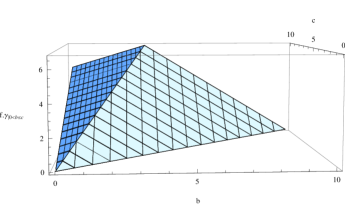
Figure 4: Piecewise linear function to be minimized by a plane.

Putting it all together we obtain the final linear expression that bounds $f.\gamma$ from below and it is in terms of the original predicates:

$$f.\gamma\geq(\tfrac{c_{2}+1}{2}c+\tfrac{1-c_{2}}{2}b)[\phi_{2}]+(\textstyle{\sum}i:[1..6]\mid i\neq 2\mbox{\raisebox{1.72218pt}{\tiny$\>\;\bullet\;\>$}}(1c+0b+0)[\phi_{i}])\enspace.$$

Note that doing this we comply with Eq. 7, and this in turn implies that $f^{\sharp}$ is a b-abstraction. We explicitly write down $f^{\sharp}$ and iterate it up-to fixed point convergence in Table 2. As expected, $\phi_{4},\phi_{5},\phi_{6}$ do not contribute in the fixed point computation since $0\leq c$ is a program invariant, so we do not include them:

$$f^{\sharp}.((c_{1},b_{1},a_{1}),(c_{2},b_{2},a_{2}),(c_{3},b_{3},a_{3}))\triangleq((1,0,0),(\tfrac{c_{2}+1}{2},\tfrac{1-c_{2}}{2},0),(1,0,0))\enspace.$$

	Coefficients
Iter.	($c_{1}$, $b_{1}$, $a_{1}$)	($c_{2}$, $b_{2}$, $a_{2}$)	($c_{3}$, $b_{3}$, $a_{3}$)
0	(0, 0, 0)	(0, 0, 0)	(0, 0, 0)
1	(1, 0, 0)	(0.5, 0.5, 0)	(1, 0, 0)
2	(1, 0, 0)	(0.75, 0.25, 0)	(1, 0, 0)
3	(1, 0, 0)	(0.875, 0.125, 0)	(1, 0, 0)
4	(1, 0, 0)	(0.9375, 0.0625, 0)	(1, 0, 0)
5	(1, 0, 0)	(0.96875, 0.03125, 0)	(1, 0, 0)
6	(1, 0, 0)	(0.984375, 0.015625, 0)	(1, 0, 0)
7	(1, 0, 0)	(0.9921875, 0.0078125, 0)	(1, 0, 0)
⋮	⋮	(1, ⋮	⋮
55	(1, 0, 0)	(1, 0, 0)	(1, 0, 0)

Table 2: Iteration for the martingale.

We can see $f^{\sharp(i)}.\bot_{\sharp}\Rrightarrow^{\sharp}f^{\sharp(i+1)}.\bot_{\sharp}$, so the under approximation $\gamma.(f^{\sharp(i+1)}.\bot_{\sharp})$ tends from below to $(\textstyle{\sum}i:[1..6]\mbox{\raisebox{1.72218pt}{\tiny$\>\;\bullet\;\>$}}(1c+0b+0)[\phi_{i}])=c$.

The initialization $c,b:=C,1$ does the rest obtaining a lower bound on the expected remaining capital, that is precisely $C$. It can be proven that $c$ is a prefix point of $f$ (in fact it is a fixed point), and using Theorem 4.2 (2), we establish $\mu.f=c$, therefore our approximation is exact. Moreover, as the program is purely probabilistic, $C$ is the expectation of $c$ with respect to $P$.

6 Aims and conclusions

This paper presents a technique for computing the expectation of unbounded random variables tailored to performance measures, like expected number of rounds of a probabilistic algorithm or expected number of detections in anonymity protocols. Our method can check quantitative linear properties on any denumerable state space using iterative backwards fixed point calculation.

Perhaps the main drawback of the method is that it is semi-computable but it covers cases where previous work cannot be applied (geometric distribution, martingales). Besides, it seems hard to bound expectations of programs syntactically since a minor (linear) modification in the geometric distribution algorithm leads to a unbounded expectation for a program that halts with probability $1$.

In future work we would like to build tool support for our approach. This would involve, among other tasks, the mechanization of the weakest pre-expectation calculus in the abstract domain, as well as the maximization problem that involves computing a lower linear function in each iteration. As our technique works on linear domains, this later task would be easily solved by known linear programming techniques.

We also plan to analyze more complex programs. The Crowds anonymity protocol modeled as in [22] is a good candidate for our automatic quantitative program analysis, since its essential anonymity properties are expressed as the expected number of times the message initiator is observed by the adversary with respect to the observations obtained for the rest of the crowd. It is also planned to reproduce the results of Rabin and Lehmann’s probabilistic dining-philosophers algorithm [17].

Acknowledgements. We would like to thank Pedro D’Argenio for his support in this project, as well as Joost-Pieter Katoen for handing us an early draft of [15].

References

- [1]
- [2] C. Baier, P.R. D’Argenio & M. Größer (2006): Partial Order Reduction for Probabilistic Branching Time. Electr. Notes Theor. Comput. Sci 153(2), pp. 97–116.
- [3] A. Bianco & L. De Alfaro (1995): Model Checking of Probabilistic and Nondeterministic Systems. Lecture Notes in Computer Science 1026, pp. 499–513.
- [4] O. Celiku (2006): Mechanized Reasoning for Dually-Nondeterministic and Probabilistic Programs. Ph.D. thesis, TUCS.
- [5] M.A. Colon & T.E. Uribe (1998): Generating Finite-State Abstractions of Reactive Systems Using Decision Procedures. In: Proc. 10 Int. Conf. on Computer Aided Verification, Lecture Notes in Computer Science 1427, Springer-Verlag, pp. 293–304.
- [6] P. Cousot & R. Cousot (1977): Abstract Interpretation: A Unified Lattice Model for Static Analysis of Programs by Construction or Approximation of Fixpoints. In: 4th POPL, Los Angeles, CA, pp. 238–252.
- [7] B.A. Davey & H.A. Priestley (1990): Introduction to Lattices and Order. Cambridge University Press.
- [8] J. Desharnais, F. Laviolette & A. Turgeon (2009): A Demonic Approach to Information in Probabilistic Systems. In: CONCUR 2009: Proceedings of the 20th International Conference on Concurrency Theory, Springer-Verlag, Berlin, Heidelberg, pp. 289–304.
- [9] S. Graf & H. Saïdi (1997): Construction of Abstract State Graphs with PVS. In: O. Grumberg, editor: Proc. 9th International Conference on Computer Aided Verification (CAV’97), Lecture Notes in Computer Science 1254, Springer-Verlag, pp. 72–83.
- [10] H. Hansson & B. Jonsson (1994): A logic for reasoning about time and probability. Formal Aspects of Computing 5(6), pp. 512–535.
- [11] H. Hermanns, B. Wachter & L. Zhang (2008): Probabilistic CEGAR. In: A. Gupta & S. Malik, editors: Computer Aided Verification, 20th International Conference, CAV 2008, Princeton, NJ, USA, July 7-14, 2008, Proceedings, Lecture Notes in Computer Science 5123, Springer, pp. 162–175.
- [12] A. Hinton, M.Z. Kwiatkowska, G. Norman & D. Parker (2006): PRISM: A Tool for Automatic Verification of Probabilistic Systems. In: H. Hermanns & J. Palsberg, editors: Tools and Algorithms for the Construction and Analysis of Systems, 12th International Conference, TACAS 2006, Lecture Notes in Computer Science 3920, Springer, pp. 441–444.
- [13] J. Hurd, A.K. McIver & C.C. Morgan (2005): Probabilistic guarded commands mechanized in HOL. Theor. Comput. Sci 346(1), pp. 96–112.
- [14] H. Jifeng, K. Seidel & A.K. McIver (1997): Probabilistic models for the guarded command language. Science of Computer Programming 28(2–3), pp. 171–192.
- [15] J.P. Katoen, A.K. McIver, L.A. Meinicke & C.C. Morgan (2009): Linear-invariant generation for probabilistic programs. Journal of Symbolic Computation Submitted.
- [16] D. Kozen (1983): A probabilistic PDL. In: STOC ’83: Proceedings of the fifteenth annual ACM symposium on Theory of computing, ACM, New York, NY, USA, pp. 291–297.
- [17] A.K. McIver (2002): Quantitative Program Logic and Expected Time Bounds in Probabilistic Distributed Algorithms. TCS: Theoretical Computer Science 282.
- [18] A.K. McIver, C.C. Morgan & C. Gonzalia (2009): Probabilistic Affirmation and Refutation: Case Studies. In APV 09: Symposium on Automatic Program Verification, Río Cuarto, Argentina.
- [19] M.W. Mislove, A.W. Roscoe & S.A. Schneider (1993): Fixed Points Without Completeness. Theoretical Computer Science 138, pp. 138–2.
- [20] D. Monniaux (2000): Abstract Interpretation of Probabilistic Semantics. In: J. Palsberg, editor: SAS, Lecture Notes in Computer Science 1824, Springer, pp. 322–339.
- [21] C.C. Morgan & A.K. McIver (2004): Abstraction, Refinement and Proofs for Probabilistic Programs. Monographs in Computer Science. Springer.
- [22] V. Shmatikov (2004): Probabilistic analysis of an anonymity system. Journal of Computer Security 12(3-4), pp. 355–377.
- [23] M. Vardi (1985): Automatic Verification of Probabilistic Concurrent Finite-State Programs. In: focs85, pp. 327–338.
- [24] B. Wachter, L. Zhang & H. Hermanns (2007): Probabilistic Model Checking Modulo Theories. In: QEST, IEEE Computer Society, pp. 129–140.