Performance Evaluation of Components Using a Granularity-based Interface Between Real-Time Calculus and Timed Automata

Abstract

To analyze complex and heterogeneous real-time embedded systems, recent works have proposed interface techniques between real-time calculus (RTC) and timed automata (TA), in order to take advantage of the strengths of each technique for analyzing various components. But the time to analyze a state-based component modeled by TA may be prohibitively high, due to the state space explosion problem. In this paper, we propose a framework of granularity-based interfacing to speed up the analysis of a TA modeled component. First, we abstract fine models to work with event streams at coarse granularity. We perform analysis of the component at multiple coarse granularities and then based on RTC theory, we derive lower and upper bounds on arrival patterns of the fine output streams using the causality closure algorithm of [3]. Our framework can help to achieve tradeoffs between precision and analysis time.

1 Introduction

Modern real-time embedded systems are increasingly complex and heterogeneous. They may be composed of various subsystems, and it is a general practice that some of the subsystems may be power-managed [6], in order to reduce energy consumption and to extend the system life time. Such a subsystem may have multiple running modes. A mode with lower power consumption also implies lower performance levels. Due to real-time requirements, it is thus critical to analyze the system timing performance, but the complexity of this analysis is challenging, especially when it is scaled to large and heterogeneous systems.

Compositional analysis techniques have been presented as a way of tackling the complexity of accurate performance evaluation of large real-time embedded systems. Examples include SymTA/S (Symbolic Timing Analysis for Systems) [10] and modular performance analysis with real-time calculus (RTC) [8]. Various models have also been proposed to specify and analyze heterogeneous components [15]. Each analysis techniques have their own particular strengths and weaknesses. For example, SymTA/S or RTC based analysis can provide hard lower/upper bounds for the best-/worst-case performance of a system, and has the advantage of short analysis time. But typically, they are not able to model complex interactions and state-dependent behavior and can only give very pessimistic results for such systems. On the other hand, state-based techniques, e.g. timed automata (TA) [4], construct a model that is more accurate, and can determine exact best-/worst-case results. But they face the state explosion problem, leading to prohibitively high analysis time and memory usage even for a system with reasonable size.

Efforts have been paid to couple different approaches [16, 11, 18, 2], e.g. to combine the functional RTC-based analysis with state-based models. The most general ones are based on interfacing RTC with another existing formalism: in [17], an interfacing technique is proposed to compose RTC-based techniques with state-based analysis methods using event count automata [9]. A tool called CATS [7] is just at the beginning of its development. It allows modeling a component using TA within a system described by RTC. A variant of the approach is described in [12], which restricts to convex and concave curves, but potentially uses less clock and may therefore scale better.

In this paper, we follow the line of recent development in interfacing between RTC and state-based models done in CATS, and focus on speeding up the analysis for a power-managed component (PMC) modeled by TA. We adapt the framework to analyze event streams at different granularities. This implies the ability to design the component to be analyzed at coarser granularities: the translation of the component from one granularity to another has to be made automatic. To do so, we focus on a class of timed automata of interest that we call M-TA, on which the translation is possible. M-TA model power-managed components, characterized with different modes of computation. We then define a schema of translation at coarser granularity. The schema is formally proven and the whole approach is validated with experimentation: we show that our abstracted model scales far better than the fine-granularity one, with a reasonable loss of precision.

Organization of the paper: in the next section 2, we detail the implementation of the existing interfacing techniques between RTC and TA. In section 3, we give an overview of the framework for granularity-based interfacing and section 4 formally details the granularity change. In section 5, we discuss our targeted PMC, and its fine and coarse TA models; and in section 6 we present some experimental validations. Finally, we make a conclusion and present future work in section 7.

2 Interfacing Timed Automata and Real-Time Calculus

Real-Time Calculus (RTC).

The Real-Time Calculus (RTC) [19] is a framework to model and analyze heterogeneous system in a compositional manner. It relies on the modeling of timing properties of event streams and available resources with curves called arrival curves and service curves. A component can be described with curves for its input stream and available resources and some other curves for the outputs. For already-modeled components, RTC gives exact bounds on the output stream of a component as a function of its input stream. This result can then be used as input for the next component.

An arrival curve is an abstraction to represent the set of event streams that can be input to (resp. output from) a component; it is expressed as a pair of curves $\xi=(\xi^{L},\xi^{U})$. For $k\geq 0$, $\xi^{L}(k)$ and $\xi^{U}(k)$ respectively provide for any potential stream the lower and upper bounds on the length of the time interval during which any $k$ consecutive events can arrive. Let $t_{i}$ denote the arrival time of the $i$-th event; $t_{i}$ may be real (we use continuous time) but the number of events that occurs at $t_{i}$ is discrete (it is represented by a natural number); we have $\xi^{L}(k)\leq t_{i+k}-t_{i}\leq\xi^{U}(k)$ for all $i\geq 0$ and $k\geq 0$.

Similarly, the processing capacity of a component is specified by a service curve $\psi=(\psi^{L},\psi^{U})$. The length of the time to process any $k$ consecutive events for any potential stream is at least $\psi^{L}(k)$ and at most $\psi^{U}(k)$.

Notice that, in the RTC theory, an arrival curve $\alpha=(\alpha^{L},\alpha^{U})$ (resp. service curve $\beta$) is usually expressed in terms of numbers of events per time interval. In this paper, we express the arrival curves ($\xi$) and service curves ($\psi$) in terms of length of time interval, in order to explain better our work. Actually, $\xi$ is a pseudo-inverse of $\alpha$, satisfying $\xi^{U}(k)=\min_{\Delta\geq 0}\{\Delta|\alpha^{L}(\Delta)\geq k\}$ and $\xi^{L}(k)=\max_{\Delta\geq 0}\{\Delta|\alpha^{U}(\Delta)\leq k\}$ (same for $\beta$ and $\psi$).

Timed Automata (TA).

A timed automaton [4] is a finite-state machine extended with clocks. A clock measures the time elapsed since its last reset and all clocks increase at the same rate. Figure 3(b) shows an example. States are labelled by invariants and transitions by guards and clock resets (e.g. $\mathbf{t}\leftarrow 0$). Invariants and guards are conjunctions of lower and upper bounds on clocks and differences between clocks. The automaton can only let time elapse in a state whenever the invariant evaluates to true. A transition may be triggered when the guard evaluates to true and some clocks are reset. Timed automata may be synchronized via binary rendez-vous: for example, the self-loop transition around Counting sends the signal produce? This means that the transition cannot be fired unless the automaton receives at the same instant the signal produce! from another one. Furthermore, we use UPPAAL TA syntax and extensions [5], such as integer counters (e.g. $cost$).

Interfacing TA and RTC

In the following, we show the techniques from CATS [7] for interfacing TA and RTC. The motivation comes from the fact that some components may not be accurately modeled with RTC tools. The idea is then to use TA for the component model, but to be nevertheless able to consider arrival and service curves to characterize inputs and outputs of the system. This implies the use of adapters, as shown in Figure 1, connecting RTC curves (which describe a set of event streams) and the TA (which inputs or outputs a single event stream). From RTC curves to TA, we use a generator that inputs events into the component such that the event stream satisfies the input curve $\hat{\xi}$. From TA to RTC, the component outputs events that feed an observer which measures the smallest and largest time interval between events, to compute the output curve $\breve{\xi}$. Both generators and observers are timed automata; they are composed with the timed automaton component and the tool UPPAAL CORA [5] is used to verify the whole. Notice that this framework is convenient whatever be the computational model used for the component (see e.g. ac2lus [2]).

Figure 1: Interfacing RTC and TA

In all this work, RTC curves are assumed to be given by a finite set of $N$ points, namely, $(\rho^{L},\rho^{U})$ are defined by the points $(\rho^{L}(i),\rho^{U}(i))$, for $i\in[1:N]$.

Generator.

The goal for the generator is, given an input arrival (resp. service) curve, to be able to generate any event stream that satisfies this curve, and only these ones. Figure 2 shows the TA model $Generator(\rho^{L},\rho^{U},\text{\bf signal})$ which non deterministically generates a sequence of signals called signal! that satisfies $(\rho^{L},\rho^{U})$.

The main idea is to reset a clock whenever an event is emitted. As we need to check any $N$ successive events, we need to memorize only $N$ clocks, that we declare in a circular clock array $\mathbf{y}$ of size $N$. $\mathbf{y}[k\%N]$ represents the time elapsed since the event $k$ has occurred. We note $\lambda$ the index of the next event to be generated: then we have to check that the $N$ events before $\lambda$ comply with the curve. The index of those events is given by the function $getIdx(i)\rightarrow(\lambda-i+N)\%N\quad(1\leq i\leq N)$. Note that at the beginning, less than $N$ events have been emitted: we introduce a bounded counter $\theta$, from $0$ to $N$ that represents the actual number of events to be considered. The constraints that satisfy the curves are then expressed as:

$$(Check\_Upper) \mathbf{y}[getIdx(i)]\leq\rho^{U}(i),\forall i\in[1:\theta]$$

$$(Check\_Lower) \mathbf{y}[getIdx(i)]\geq\rho^{L}(i),\forall i\in[1:\theta]$$

$(Check\_Upper)$ expresses an invariant on how much time can elapse (i.e. when an event must be generated), whereas $(Check\_Lower)$ qualifies the date from which a new event may be emitted, checked before emitting a new signal.

Figure 2: $Generator(\rho^{L},\rho^{U},\text{\bf signal})$: model of a generator from RTC to TA.

Observer.

To compute the output curve $(\rho^{L},\rho^{U})$, we use a model checking tool with cost optimal reachability analysis [5]. An observer is used to capture the arrival patterns of an event stream: Figure 3(a) computes lower and upper bound for a stream of produce! events and for a window of $K$ events, namely $(\rho^{L}(K),\rho^{U}(K))$.

The observer non-deterministically transits from the initial state Idle to Counting: this decides the beginning of the window to be observed. The counter $\eta$ records the number of produce! since the entry in Counting. When reaching the state Stop, $K$ produce! events have been emitted.

The cost for an execution corresponds to the time spent in the Counting state (no cost on transition, cost rate of 1 for Counting – marked as a grey state in the figure, cost rate of 0 for the other states). Therefore, the cost when reaching the state Stop is equal to the time for emitting $K$ events. With a verification engine able to compute the minimum and maximum cost for reaching Stop, this provides $\rho^{L}(K)$,since the $K$ consecutive events were chosen non-deterministically. The computation has to be launched $N$ times (for $K=1$ to $N$) to obtain all the points of the curves.

Since the tool we use can not compute a maximum, we use a variant model of the observer shown in Figure 3 (b) for computing the maximum and obtaining $\rho^{U}(K)$. The principle of the timed automata is the same as the former but it measures the number of events (counter $cost$) that can be emitted during an interval of length $\Delta$ (clock $\mathbf{t}$). When minimizing the cost, this provides $\alpha^{U}(\Delta)$. Then, $\rho^{U}$ is computed as the pseudo-inverse of $\alpha^{U}$.

(a) $Observer(K,\text{\bf produce})$

(b)

Figure 3: (a) Model of the observer and (b) its varied model.

How to obtain output arrival curves?

We show here how to instantiate the timed automata described above to compute an output arrival curve $\breve{\xi}$ given the input arrival curve $\hat{\xi}$, the input service curve $\psi$ and a component modeled as a timed automaton. The input event stream is labeled by signals req and is given by $Generator(\hat{\xi}^{L},\hat{\xi}^{U},\text{\bf req})$. The input service stream is labelled by signals serv and is generated by $Generator(\psi^{L},\psi^{U},\text{\bf serv})$. We assume that the component inputs req and serv signals and emits produce signals. The output event stream is then analyzed by $Observer(K,\text{\bf produce})$. Those four automata are synchronized and a verification engine is used, to obtain all the points $(\breve{\xi}^{L}(K),\breve{\xi}^{U}(K))$, for $K=1$ to $N$.

Note that the whole model involves two clock arrays of size $N$ (length of the curve); it also involves two $N$-counters per generator plus one $N$-counter for the observer. The size of the model, hence, heavily depends on the number of events to be considered.

3 The Granularity-based Interfacing Framework

Motivations.

When model-checking non-trivial systems of TA, one quickly faces the well-known state-explosion problem. Generally speaking, this mainly comes from two sources: clocks and counters. Counters are handled as discrete states in the proof engine and clocks involve the dimensions of the polyhedra (zones) to be computed. As stated above, the CATS approach proposes to model-check (with cost optimization) a model where the numbers of clocks and the order of magnitude of counters are heavily linked with the number of events to be considered and so is the cost to compute the results. Applied to non-trivial components the approach may thus fail to provide any result.

By grouping the events, and refraining from looking at them individually, we can reduce the amount of events analysis and thus both the size of counters and the number of clocks: we can hence get dramatic improvements on the performance. We talk about fine events to designate the real events of the system and we group them into coarse events which intuitively represent a packet of $g$ fine events, where $g$ is called the granularity of the abstraction. Modeling the system to work with coarse events instead of fine events divides the length of the arrival curve $\hat{\xi}$ and the number of events $N$ to store in buffers by $g$. By changing the value of $g$, one can trade performance for accuracy.

Framework.

We propose a formal framework of granularity-based interfacing between RTC and TA performance models. The generators for service and arrival curves, the component model and the observer for the output arrival curve deal all with coarse events, which speeds up the analysis.

As we change the granularity, all TA models involved in the framework have to be adapted to deal with the coarse events. For the generators and the observers, this is quite straightforward, but abstracting an arbitrary TA component to a coarse-granularity one would be hard, if at all possible. We focus on a particular class of timed automata that we call M-TA (for “Mode-based Timed-Automata”) for which we propose an automatic translation scheme from fine event M-TA to coarse event M-TA. For simplicity of the notations, we define the class of M-TA with an abstract syntax, the semantics of an M-TA being given by the corresponding TA. This is illustrated by (a) and (b) in Figure 4. The correctness of the approach relies on the fact that the coarse-grain translation of an M-TA is an accurate abstraction, in the sense that the lower and upper coarse output curves, analyzed from the coarse model, always provide lower and upper bounds on the lower and upper fine curves, which would be obtained from the original fine model. This is proved once and for all for the translation scheme.

When analyzing a coarse model, we get a pair of coarse output arrival curves that already provides lower and upper bounds on the arrival patterns of the output stream at fine granularity, by applying a simple rescaling. But it is possible to derive tighter fine output curve, running the analysis at different granularity levels $g_{1}...g_{m}$. The resulting coarse output curves $\breve{\xi}_{g_{1}}...\breve{\xi}_{g_{m}}$ are then combined (see Figure 4.(c)) using the causality closure [3] property of RTC curves. This results in a tighter output arrival curve ($\tilde{\xi}$) at the fine granularity which is tighter than the naive combination of the curves but still equivalent to it.

To the best of our knowledge, no existing work deal with a granularity-based scheme with formal validation on the abstraction. The proposed framework complements the recent works on interfacing between RTC and TA models.

Figure 4: The framework of granularity-based interfacing.

4 Changing the Granularity

Definitions and Notations.

We denote a specific stream at the fine granularity as $\tau=(t_{0})t_{1}t_{2}...$ and a specific coarse stream to be $\top=(T_{0})T_{1}T_{2}...$. $t_{i}$ (resp. $T_{i}$) denotes the arrival time of the $i$-th fine (resp. coarse) event $\varepsilon_{i}$ (resp. $\mathcal{E}_{i}$) for $i\geq 1$. $t_{0}=T_{0}=0$ denotes the origin of time. $\hat{\top}$ and $\hat{\tau}$ denote the input, while $\breve{\top}$ and $\breve{\tau}$ denotes the output stream.

As illustrated in Figure 5, we can abstract a fine stream to a coarse one at some granularity $g$, by regarding $g$ consecutive fine events as a coarse one. A fine stream $\tau$ is a refinement of a coarse one $\top$ if $T_{i}$ is equal to $t_{gi}$ for $i\geq 0$, i.e. if it is sampling the fine stream every $g$ events. A coarse stream $\top$ at granularity $g$ is an abstraction of a fine stream if $t_{gi}=T_{i}$ for $i\geq 0$, the other $t_{k}$ being chosen arbitrarily, with $t_{k+1}\geq t_{k}$. It is easy to see that a coarse stream $\top$ can be refined to a fine stream $\tau$ if and only if $\tau$ can be abstracted to $\top$.

Figure 5: Illustration of a fine and coarse stream with $g=3$.

How to obtain coarse output arrival curves?

We now show how to use the interfacing between RTC and TA (Section 2) to compute output arrival curves at coarser granularity. The input arrival (resp. service) curve $\hat{\xi}$ (resp. $\psi$) is given for fine events. To obtain the input arrival (resp. service) curve for coarse events at granularity $g$, $\hat{\xi_{g}}$ (resp. $\psi_{g}$), we use a sampler. From $\hat{\xi}$ it produces $\hat{\xi_{g}}$ such that $\hat{\xi}_{g}(k)=\hat{\xi}(gk)$ for $k\geq 0$ (the definition of $\psi_{g}$ is exactly the same). Indeed, it is easy to see that the arrival (resp. service) pattern for the coarse input streams are lower and upper bounded by $\hat{\xi}(gk)$ (resp. $\psi(gk)$) for all $k\geq 0$. Notice that this abstraction from fine input streams $\hat{\tau}$ to coarse ones $\hat{\top}$ at granularity $g$ implies to lose information about every fine events but the ones at $gi$, $\varepsilon_{gi}$.

To compute a coarse output arrival curve $\breve{\xi_{g}}$, we then proceed as before: a generator is used for both the arrival curve $\hat{\xi_{g}}$ and the service curve $\psi_{g}$; and observers are used to compute the result using model-checking with cost optimality. Nevertheless, between them, the component still has to be adapted. Indeed, it was designed to proceed on fine events and needs to be abstracted to work on coarse input streams. In the sequel, we note $\mathcal{P}_{0}$ the fine component and $\mathcal{P}_{C}$ its coarse abstraction. This transformation from $\mathcal{P}_{0}$ to $\mathcal{P}_{C}$ may be hard, if possible and we define a particular class of interest, called M-TA, for which we provide an automatic transformation scheme. This is the topic of the following section. Notice that such an abstraction introduces non-determinism in the coarse component. For example, when the triggering condition of a transition depends on a number of events, the coarse grain component cannot know exactly the time at which the transition is triggered.

Validation.

To validate the proposed framework, one has to guarantee that the coarse models provide accurate abstraction of the fine models. The proof can be made on every parts of the model but the component, since the TA are given. For the component, we exhibit a proof obligation that has to be guaranteed to validate the whole framework. This proof obligation states that the coarse component $\mathcal{P}_{C}$ should exhibit at least all the behaviors that the fine component $\mathcal{P}_{0}$ can produce. Formally, it should satisfy the following property.

Definition 1

Let $\hat{\tau}=(\hat{t}_{0})\hat{t}_{1}\hat{t}_{2}...$ ($\breve{\tau}=(\breve{t}_{0})\breve{t}_{1}\breve{t}_{2}...$) be any fine event stream that is an input to (the corresponding output stream produced from) $\mathcal{P}_{0}$. We say that $\mathcal{P}_{C}$ is a correct abstraction of $\mathcal{P}_{0}$ iff(def) there always exists some coarse event stream $\hat{\top}$ ($\breve{\top}$) that can be an input to (the corresponding output stream produced from) $\mathcal{P}_{C}$, such that $\hat{\top}$ ($\breve{\top}$) can be refined to $\hat{\tau}$ ($\breve{\tau}$).

Proof Obligation 1

Prove that $\mathcal{P}_{C}$ is a correct abstraction of $\mathcal{P}_{0}$.

We will show later that the TA generated by our translation verify this proof obligation. Any other way to generate coarse TA that satisfy it could be used in the framework.

The correctness of the abstraction implies that we can derive a valid coarse output curve $\breve{\xi}_{g}$, by analyzing $\mathcal{P}_{C}$.

Lemma 1

If Proof Obligation 1 is satisfied, it is guaranteed that the analyzed $\breve{\xi}_{g}^{L}(k)$ and $\breve{\xi}_{g}^{U}(k)$ provide lower and upper bounds on $\breve{\xi}^{L}(gk)$ and $\breve{\xi}^{U}(gk)$ respectively for $k\geq 0$.

Sketch of proof: it follows from Proof Obligation 1 that, for any fine output stream $\breve{\tau}$ from $\mathcal{P}_{0}$, there always exists a coarse output stream $\breve{\top}$ such that $\breve{\top}$ can be refined to $\breve{\tau}$. It follows that the production time of the ($g\times k$)-th fine event in $\breve{\tau}$ is equal to that of the $k$-th coarse event in $\breve{\top}$. It is then easy to show that $\breve{\xi}_{g}^{L}(k)\leq\breve{\xi}^{L}(gk)$ and $\breve{\xi}_{g}^{U}(k)\geq\breve{\xi}^{U}(gk)$.

How to combine multiple coarse curves to obtain a fine one?

The above paragraphs show how to obtain a coarse pair of output curves at a given granularity and prove their accurateness. We now propose to conduct multiple runs of analysis at different granularities $g_{1},...,g_{m}$, and show how to combine them to obtain a valid fine pair of output curves. The coarse output arrival curve at granularity $g_{i}$ is noted $\breve{\xi}_{g_{i}}$ ($i=1,...,m$) and we denote by $\breve{\xi}^{U}$ and $\breve{\xi}^{L}$ the optimal fine output arrival curves. Due to Lemma 1, we have $\breve{\xi}^{U}_{g_{i}}(k)\geq\breve{\xi}^{U}(kg_{i})$ and $\breve{\xi}^{L}_{g_{i}}(k)\leq\breve{\xi}^{L}(kg_{i})$ for $k\geq 0$.

Therefore, a first approximation of $\breve{\xi}^{U}$ (resp. $\breve{\xi}^{L}$) is to take the minimal (resp. maximal) obtained values for different granularities: $\breve{\xi}^{U}_{combined}(n)=\min_{kg_{i}\geq n}\{\breve{\xi}^{U}_{g_{i}}(k)\}$. But this curve is not necessarily the tightest we can find.

Suppose, for example, that we obtain output curves $\breve{\xi}_{2}$ and $\breve{\xi}_{3}$ after analyzing $\mathcal{P}_{C}$ with $g=2,3$. We can get on $\breve{\xi}(1)$ some tighter bounds than the minimum of $\breve{\xi}_{2}^{U}(1)$, $\breve{\xi}_{3}^{U}(1)$ as follows. Let $\tau=t_{0}t_{1}t_{2}...$ denote the trace of the fine output stream, ($t_{i}$ denotes the production time of the $i$-th fine event $\varepsilon_{i}$), with $t_{0}=0$. Recalling that $\breve{\xi}^{L}(k)$ and $\breve{\xi}^{U}(k)$ are defined to be lower and upper bounds on the length of the time interval during which any $k$ consecutive events are output, for any $i\geq 0$, we have $\breve{\xi}^{L}(2)\leq t_{i+3}-t_{i+1}\leq\breve{\xi}^{U}(2)$ and $\breve{\xi}^{L}(3)\leq t_{i+3}-t_{i}\leq\breve{\xi}^{U}(3)$. We can thus derive constraints on time interval of length 1:

$$\breve{\xi}^{L}(3)-\breve{\xi}^{U}(2)\leq t_{i+1}-t_{i}\leq\breve{\xi}^{U}(3)-\breve{\xi}^{L}(2)$$

Hence, a better valid bound for the time interval between any two events is given by

$$\left[\max\left\{\breve{\xi}^{L}(1),\breve{\xi}^{L}(3)-\breve{\xi}^{U}(2)\right\},\min\left\{\breve{\xi}^{U}(1),\breve{\xi}^{U}(3)-\breve{\xi}^{L}(2)\right\}\right]$$

Other linear constraints can be used to derive constraints in such a flavor. But, we actually use the causality closure algorithm given in [14] which refine an arbitrary pair of curves to the optimal equivalent pair of curves (provided a slight adaptation of the algorithm for finite curves to work with pseudo-inverse of the curves). This algorithm is based on the notion of deconvolution, which is basically a generalization of the above example by taking all the possible values instead of just $2$ and $3$ as in the example.

5 Application to Power Managed Components

The systems we target to define an automatic translation from fine to coarse models are energy-aware, or “power-managed”. They have different modes of operations, in which their performance and energy consumption are defined. Most computers and embedded systems today possess energy-saving modes; for example, CPUs can have dynamic voltage and frequency scaling (DVFS) and sensors in a network can switch their radio on and off.

5.1 Models of PMC

We consider power-managed components (PMC) as systems with different modes of operation, each mode owning a pair of service curves. The system can transit from a mode to another upon various conditions. The minimal requirements to model non-trivial systems is:

1. by receiving an explicit synchronization from another component

2. after a given timeout (typically, systems go to a hibernation state only after spending some time in an idle state),

3. when the buffer fill level exceeds a certain threshold (to switch to a resource-intensive one when the system is overloaded),

4. when the buffer fill level gets below a threshold (typically, go to an energy-saving state when the buffer is empty).

Also, we need a way to force the system to stay in a given mode for a minimum amount of time (for example, to model a transition between two modes that physically takes some time). This is modeled by modifying the last two conditions to enable them only when the time spent in the current mode is greater than some constant.

Graphical Syntax to Describe PMC.

From these requirements, we define the class of automata M-TA, and give a graphical syntax for it. The description is based on an enumeration of modes, each mode $M_{i}$ being associated with a pair of service curves $\psi_{i}=(\psi^{L}_{i},\psi^{U}_{i})$; it is restricted to how the PMC can evolve from mode to mode. To handle the events to be computed, we suppose that the PMC is equipped with a buffer at its entry. We note $q$ the counter for the buffer fill level: in each mode $M_{i}$ it is constrained to be within some lower and upper bounds $b_{i}^{U}$ and $b_{i}^{L}$. A mode $M_{i}$ is also equipped with time constants $L_{i},U_{i}$ which represent the lower and upper time the component can stay in the mode; we use the clock $\mathbf{x}$ to measure this time: it is reset when entering a mode and checked against the bounds when going out. Figure 6 shows a descriptive model of the PMC with all the possible mode changes ((1)..(4), using the same numbering as above). We believe that our work can be easily extended to other cases of mode switch.

Figure 6: M-TA: 4 kinds of transitions between modes

Semantics of M-TA.

Given a PMC described by a M-TA, we give its semantics in terms of the TA it represents. Using the same convention as before, a PMC receives events through the signal req? from the generator and emits produce! at its output. Internally, we translate the M-TA using two synchronized TA: the first, called Processing Element (PE), controls the mode switches and the second, called Service Model (SM) models the computation resources for each mode. The PE and the SM are strongly synchronized: the PE emits signals Syn_ij! whenever transiting from mode $M_{i}$ to mode $M_{j}$ and the SM changes its behavior accordingly. The SM has the same discrete structure as the abstract syntax. It uses one instance of the generator described in section 2 per mode $M_{i}$ (i.e. per state), $Generator(\psi_{i}^{L},\psi_{i}^{U},\text{\bf{serv}})$ which emits serv! whenever the PMC is able to process an event. This serv! signal is then transmitted to the PE, which decrements its backlog $q$ and emits a produce! (received by the observer).

Similarly, each time the PE receives an event to be processed via the signal req? (received from the generator that models the input arrival curves) this increments the backlog $q$. Before further detailing the implementation of the PE in terms of timed automata, we define a shortcut syntax for a state in Figure 7. The interval $[b^{L},b^{U}]$ specified on the state $S$ means that the system can stay in $S$ all along the buffer fill level $q$ is within this range. The clock invariant $\mathbf{x}\leq U$ has the usual meaning. This shortcut enables the model to be complete with respect to the incoming events req? and serv?.

REQ means: $\{$ req? $q$++; $\}$

SERV means: if ($q$>0) $\{$ serv? $q$--; produce! $\}$ else $\{$ serv? $\}$

Figure 7: Simplified notation of a state of the PE

Figure 8 shows, for the PE, the translation of the 4 kinds of transitions of the M-TA in Figure 6 into plain TA; notice that it only expands the single mode $M_{i}$. This mode is implemented with two states $S_{i}$ (initial state) and $S_{i1}$. $S_{i}$ is added to ensure that the PE doesn’t leave the mode before reaching its lower timing constraint $L_{i}$. When $\mathbf{x}=L_{i}$, it is time to leave $S_{i}$: either the exit condition on $q$ ($q>b^{U}_{i}$ or $q<b^{L}_{i}$) is already satisfied and the TA immediately switches to the corresponding mode ($M_{j}$ or $M_{k}$) or it transits to the state $S_{i1}$. It can stay in $S_{i1}$ while $q\in[b^{L}_{i},b^{U}_{i}]$ and $\mathbf{x}\leq U_{i}$. Whenever $q$ exceeds $b^{U}_{i}$ or falls below $b^{L}_{i}$, it switches to a new mode ($M_{j}$ or $M_{k}$). When the timeout $U_{i}$ is reached, the transition to $M_{p}$ is forced by the invariant. In both $S_{i}$ and $S_{i1}$, whenever the automaton receives a synchronization signal a?, it must immediately transit to $M_{l}$.

Figure 8: Fine TA model of the PE

5.2 PMC Models at Coarser Granularity

We now give the translation scheme from M-TAs to TA at granularity $g$ for $g>1$. This translation gives an abstraction of the original M-TA, which consumes and produces coarse events. Like in the previous section, we translate one PMC into two TA: the processing element (PE) and the service model (SM).

Coarse Service Model (SM).

Changing the granularity for the SM is done by sampling the service curves like we did in section 4. It thus still uses one $Generator(\hat{\xi}^{L}_{g}$, $\hat{\xi}^{U}_{g},\text{\bf serv})$ of Figure 2 per mode $M_{i}$ but each mode is refined into two states. When a mode switch occurs, we do not know how many fine events have been emitted since the last coarse serv! in previous mode (but it has to be within the $[0,g)$). Arriving in the new mode $M_{i}$, the SM has to wait for $k$ more fine events before emitting the next coarse serv!, $k$ being in $(0,g]$. As shown in Figure 10, we add a state $S_{trans}$ to capture this fact. The time the SM stays in this state is non-deterministically chosen within $[\psi^{L}_{i}(1),\psi^{U}_{i}(g)]$; it is measured by the clock x.

Coarse Processing Element (PE).

The coarse translation of the PE is given in Figure 9 using the notations introduced in Figure 7. The overall idea is the same as the fine model (Figure 8), but the buffer fill level, here noted $Q$, now counts coarse events instead of fine events. The state $S_{i1}$ has been split into three states $S_{i1}$, $S_{inc}$ and $S_{dec}$ whose meaning are given in the figure. This splitting is necessary because when the condition between two modes depends on a threshold $b^{U}_{i}$ or $b^{L}_{i}$ on the backlog $q$ at fine granularity, if this threshold is not a multiple of $g$, then the actual transition of the fine PMC would occur between two coarse events. We note $Y^{L}$ and $Y^{U}$ (resp. $H^{L}$ and $H^{U}$) the smallest and greatest numbers of coarse events between which the fine threshold $b^{U}_{i}$ (resp. $b^{L}_{i}$) can be reached. The explanation and the values on those constants are given Figure 9. We can therefore not determine precisely when a transition due to a threshold does occur in the fine PE, but we have to ensure in the coarse PE, due to the proof obligation 1, that it can occur at the same time as it would have in the fine PE. The coarse PE leaves the state $S_{i1}$ when one of the transitions to $M_{j}$ or $M_{k}$ can occur, and the invariants on states $S_{inc}$ and $S_{dec}$ say when the transition must occur. The management of synchronization events (a?) and timeout ($\mathbf{x}=U_{i}$) is the same as in the fine model. For clarity, it is not drawn on the TA but described above.

Coarse thresholds: $Y^{L}=\big{\lfloor}(b_{i}^{U}+1)/g\big{\rfloor},\;Y^{U}=\big{\lceil}(b_{i}^{U}+1)/g\big{\rceil},\;H^{L}=\big{\lfloor}(b_{i}^{L}-1)/g\big{\rfloor},\;H^{U}=\big{\lceil}(b_{i}^{L}-1)/g\big{\rceil}$
Explanation on those values: let $N_{r}$ (resp. $N_{s}$) denotes the total number of coarse events req? (resp. serv?) received since the system started. Let $n_{r}$ (resp. $n_{s}$) denotes the corresponding total number of fine events. $Q$ (resp. $q$) denotes the coarse (resp. fine) buffer fill level. At any time, we have the following constraints: $gN_{r}\leq n_{r}<g(N_{r}+1)\;\text{ and }\;gN_{s}\leq n_{s}<g(N_{s}+1)$.
Since the fine and coarse buffer fill levels $q$ and $Q$ satisfy $q=n_{r}-n_{s}$ and $Q=N_{r}-N_{s}$ respectively, we deduce that $g(Q-1)<q<g(Q+1)$. This implies that $\lfloor q/g\rfloor\leq Q\leq\lceil q/g\rceil$. When $q$ is replaced with $b^{U}_{i}+1$ in the former inequation, it provides lower and upper bounds $[Y^{L},Y^{U}]$ on the value of $Q$. We can similarly derived the bounds $[H^{L},H^{U}]$.
Meaning of the states: $\mathbf{S_{i}}$: same as $S_{i}$ in the fine PE. $\mathbf{S_{i1}}$: the coarse backlog corresponds to a fine buffer fill level between $b_{i}^{L}$ and $b_{i}^{U}$. $\mathbf{S_{inc}}$ / $\mathbf{S_{dec}}$: in the fine PE, the buffer fill level may have reached $b_{i}^{U}$ / $b_{i}^{L}$.
Other transitions: 4 transitions labelled (a?,Syn_il!) from $S_{i}$, $S_{inc}$, $S_{i1}$, $S_{dec}$ to the mode $M_{l}$ and 3 transitions labelled ($\mathbf{x}=U_{i}$,Syn_ip!) from $S_{inc}$, $S_{i1}$, $S_{dec}$ to the mode $M_{p}$.

Figure 9: Simple coarse PE model

Figure 10: Simple coarse service model

Validation.

Due to the proof obligation 1, we now have to prove that the proposed simple coarse PMC provides a correct abstraction of the fine PMC.

Proof: let $\hat{\tau}=(\hat{t}_{0})\hat{t}_{1}\hat{t}_{2}...$ be any fine input stream to the fine PMC $\mathcal{P}_{0}$, and $\breve{\tau}=(\breve{t}_{0})\breve{t}_{1}...$ is the corresponding output stream. Firstly, we construct a coarse input stream $\hat{\top}=(\hat{T}_{0})\hat{T}_{1}\hat{T}_{2}...$ with $\hat{T}_{j}=\hat{t}_{gj}$ for $j\geq 0$. It is clear that $\hat{\top}$ can be refined to $\hat{\tau}$, while $\hat{\top}$ can be an input to the coarse PMC $\mathcal{P}_{C}$ due to:

$\forall j\geq k\geq 0,\hat{\xi}_{g}^{L}(j-k)=\hat{\xi}^{L}(g(j-k))\leq\hat{t}_{gj}-\hat{t}_{gk}\leq\hat{\xi}^{U}(g(j-k))=\hat{\xi}_{g}^{U}(j-k)$

Then we show how to construct a coarse output stream $\breve{\top}$ from $\mathcal{P}_{C}$ corresponding to the input stream $\hat{T}$ and which is an abstraction of $\breve{\tau}$: given the behavior of $\breve{\tau}$, we build, by induction, the behavior $\breve{\top}$ where mode switches occur at the same time in the fine and the coarse PMCs.

Firstly, when the system starts, both PMCs can enter the starting mode at the same time. Suppose now that the coarse output stream $\breve{\top}$ has been constructed until the $(A-1)$-th event, for some $A>0$, to be $(\breve{T}_{0})\breve{T}_{1}...\breve{T}_{A-1}$ with $\breve{T}_{j}=\breve{t}_{gj}$ for all $j\in[0,A-1]$; and that both $\mathcal{P}_{0}$ and $\mathcal{P}_{C}$ entered the mode $M_{i}$ at the same instant.

Let the fine PMC $\mathcal{P}_{0}$ leaves $M_{i}$ when the ($gB+n$)-th fine event produce! is processed, with $n<g$. Two cases can then happen:

Case 1: $B=A-1$. From the service model shown in Figure 10, the time to generate the next coarse event serv? is lower and upper bounded by $\psi^{L}_{i}(1)$ and $\psi^{U}_{i}(g)$ respectively. It covers all the possibility of what can happen in the fine service model. Hence, it is possible that the coarse PMC leaves $M_{i}$ at the same time as the fine one.

Case 2: $B>A-1$. In mode $M_{i}$, we continue to construct $\breve{\top}$ to be $...\breve{T}_{A-1}\breve{T}_{A}...\breve{T}_{B}$, with $\breve{T}_{j}=\breve{t}_{gj}$ for $j\in[A,B]$. Similarly to the Case 1 above, we can show that $\breve{T}_{A}$ can be an output from $\mathcal{P}_{C}$. We can also show that $\breve{T}_{A+1}...\breve{T}_{B}$ can be an output from $\mathcal{P}_{c}$, due to $\psi^{L}_{i}(g(j-A))\leq\breve{t}_{gj}-\breve{t}_{gA}\leq\psi^{U}_{i}(g(j-A))$ and $\psi^{L}_{gi}(j-A)=\psi^{L}_{i}(g(j-A))$, $\psi^{U}_{i}(g(j-A))=\psi^{U}_{gi}(j-A)$. The coarse PMC is able to leave $M_{i}$ at the same time as the fine PMC. Indeed, as shown in Figure 9, $\mathcal{P}_{C}$ may transit out from $S_{inc}$ (or $S_{dec}$) anytime before $Q$ increases to $Y^{U}+1$ (or falls below $H^{L}-1$). Hence, it is possible that $\mathcal{P}_{C}$ transits out at the same time as $\mathcal{P}_{0}$ for the case of those transitions. In other cases of transiting out, the time to transit out is same for $\mathcal{P}_{C}$ and $\mathcal{P}_{0}$, which is equal to $L_{i}$, $U_{i}$ or the time receiving the synchronization signal a?.

It is clear that the constructed coarse output stream $\breve{\top}$ is an abstraction of the fine one $\breve{\tau}$. Therefore, the proof obligation 1 is validated.

Optimization of the coarse PMC model.

This unoptimized model introduces non-determinism when mode changes occur. For example, if one knows that a mode change occurs when $q=12$, with a granularity of $g=5$, one can not capture in the coarse model the exact instant where $q$ becomes equal to 12, but only the arrival of the second and third coarse events ($T_{2}$ and $T_{3}$), which correspond to $q=10$ and $q=15$. By reusing the information we have on the service and arrival curves at the fine granularity, we can get a better estimation than $[T_{2},T_{3}]$ for the time at which the mode change occur. In the example, one can get a lower bound $x$ for the time needed to get 2 more events in the buffer: $\hat{\xi}^{U}$ says how fast the events can arrive, and $\psi^{L}$ says how fast the PMC processes them. We can compute the minimal time for which the difference between the number of events received and the number of events processed is 2. Similarly, we can get an interval $[i_{s},i_{e}]$ on the time between the mode change and the next coarse serv? event. In the TA model, this is implemented by forcing the automaton to remain in the old mode for $x$ time units after receiving the second event, and to enable the transition for the first serv? only when the time spent in the mode is in $[i_{s},i_{e}]$.

We implemented two variants of this optimization in our prototype. The first introduces a counter $\omega$ and the corresponding coarse PMC is called $\mathcal{P}_{C}$-$\omega$, and the second does all the complex computations on best and worst cases using this counter, and the corresponding coarse PMC is called $\mathcal{P}_{C}$-opt. These optimizations considerably increase the precision of the analysis. They are detailed in [13], but omitted here by lack of space.

6 Experimental Validation

Tools.

To conduct experimentations on our framework, we applied the TA modeling and verification tool UPPAAL CORA [5], to model TA and to analyze the output arrival curves by model checking. The generators and observers are written once for all, but for the PMC, the M-TA translation into TA has still to be written by hand. Running the analysis at multiple granularities and the algorithm to combine the obtained curves into the tightest one is fully automated.

An Example of PMC.

We illustrate the approach with the fine and coarse models of a simple PMC illustrating a common behavior. It runs at two modes: “sleep” and “run”. It only processes events and consumes energy in the “run” mode and switches to the power-saving “sleep” mode when its buffer is empty. To avoid switching back and forth between “run” and “sleep”, the PMC waits until its buffer fill level $q$ reaches a threshold $q_{0}$ before transiting from “sleep” to “run”. Initially the input buffer is empty (i.e. $q=0$). Figure 11 shows the model of this example PE in terms of M-TA.

Figure 11: M-TA model of the example PMC

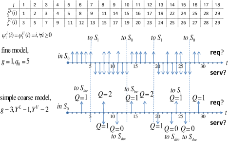
Figure 12: An illustrated flow of the example PMC

Result of the Analysis for the Example.

We show the experiments conducted on the previous example where the threshold $q_{0}$ is set to 5 (i.e. the PMC starts to run when the number of fine events in the buffer reaches 5). We first apply the translation from the M-TA to TA presented above to get the coarse and fine-grain model. Notice that, since the M-TA doesn’t exhibit all the cases of mode-changes, the translation can indeed be optimized manually (see [13]). In Figure 12, we take an example input stream and show its execution in the fine and coarse PMC models at granularity 3. It can be observed that the coarse PE always switches from $M_{0}$ to $M_{1}$ when it stays in $S_{inc}$ and switches from $M_{1}$ to $M_{0}$ when it stays in $S_{dec}$. This illustrates how the non-determinism is introduced in the coarse model.

output	analysis time at granularity $g$ [sec]
arrival	$g=1$	$g=2$			$g=3$			$g=4$
curves	$\mathcal{P}_{0}$	$\mathcal{P}_{C}$	$\mathcal{P}_{C}$-$\omega$	$\mathcal{P}_{C}$-opt	$\mathcal{P}_{C}$	$\mathcal{P}_{C}$-$\omega$	$\mathcal{P}_{C}$-opt	$\mathcal{P}_{C}$	$\mathcal{P}_{C}$-$\omega$	$\mathcal{P}_{C}$-opt
$\breve{\xi}^{L}_{g}(k)$	23674.4	56.1	62.9	223.6	7.90	12.9	189.7	0.76	1.21	28.6
$\breve{\xi^{\prime}}^{U}_{g}(k)$	411515.3	746.2	583.2	4217.7	68.6	120.9	1465.4	7.43	12.5	269.1
distance	/	4.17	2.46	0.63	5.50	2.88	0.63	9.08	5.08	1.25

Table 1: Time to compute fine and coarse output arrival curves ($\breve{\xi}^{L}_{g}$, $\breve{\xi^{\prime}}^{U}_{g}$), and the distance between coarse and fine curves, with $distance=\text{\it mean}(\text{\it mean}(\breve{\xi}^{L}(gk)-\breve{\xi}^{L}_{g}(k)),\text{\it mean}(\breve{\xi}^{U}_{g}(k)-\breve{\xi}^{U}(gk)))$ where mean is the average of all the elements for $1\leq k\leq\lfloor 24/g\rfloor$.

We now comment the results of coarse output arrival curves when running the analysis at multiple granularities $g=2,3,4$. First the input arrival curves $\hat{\xi}$ and service curves $\psi$ are sampled by taking the points of the curves having an abscissa multiple of $g$ (an illustration is given in appendix A.1). Then, using the UPPAAL CORA tool, we analyze the minimum cost to reach the Stop state of the observer model, which gives the lower output curve $\breve{\xi}^{L}_{g}(k)$ and use the variant of the observer shown in Figure 3(b) to compute $\breve{\alpha}^{U}$, which gives $\breve{\xi}^{U}_{g}$ after pseudo-inversion.

For granularity $g=4$, we compare the output curves ($\breve{\xi}^{L}_{4}$, $\breve{\xi}^{U}_{4}$) using the unoptimized PMC $\mathcal{P}_{C}$, ($\breve{\xi}^{L}_{4}$-$\omega$, $\breve{\xi}^{U}_{4}$-$\omega$) using the model with $\omega$, $\mathcal{P}_{C}$-$\omega$ and ($\breve{\xi}^{L}_{4}$-opt, $\breve{\xi}^{U}_{4}$-opt) using the optimized PMC $\mathcal{P}_{c}$-opt, as shown in Appendix A.2. It can be observed that $\mathcal{P}_{C}$-$\omega$ helps to obtain tighter coarse output curves than $\mathcal{P}_{C}$, which are further improved by $\mathcal{P}_{C}$-opt.

When analyzing the coarse output curves at each granularity, $g=2,3,4$, obtained from the optimized coarse PMC $\mathcal{P}_{C}$-opt, ($\breve{\xi}^{L}_{g}$, $\breve{\xi}^{U}_{g}$), it can be observed that $\breve{\xi}^{L}_{g}(k)$ provides a lower bound on $\breve{\xi}^{L}(gk)$ and $\breve{\xi}^{U}_{g}(k)$ provides an upper bound on $\breve{\xi}^{U}(gk)$; where ($\breve{\xi}^{L}$, $\breve{\xi}^{U}$) is the fine output curves computed from the fine PMC $\mathcal{P}_{0}$ (see Appendix A.2).

Table 1 summarizes the analysis at multiple granularities by showing the total time to compute the fine and coarse output curves ($\breve{\xi}^{L}_{g}(k)$, $\breve{\xi}^{U}_{g}(k)$) for $g=1,2,3,4$ and $k\leq\lfloor 24/g\rfloor$. It also shows the $distance$ measured between coarse and fine curves. As expected, the three models $\mathcal{P}_{C}$, $\mathcal{P}_{C}$-$\omega$ and $\mathcal{P}_{C}$-opt allow a trade-off between performance and accuracy, $\mathcal{P}_{C}$ being the fastest and less precise, and $\mathcal{P}_{C}$-opt the slowest and most precise. The granularity $g$ allows another trade-off: the coarsest models are the least precise ones and the fastest to analyze.

Finally, we experiment that applying the causality closure [3], (quadratic algorithm), to the resulting curves give information that neither of the analysis would have given alone. For example, running the analysis with $q_{0}=21$ at granularities $g=9$ and $g=10$, we get $\breve{\xi}^{U}_{10}(2)=111$ and $\breve{\xi}^{U}_{9}(2)=108$, which trivially implies $\breve{\xi}^{U}(10)\leq 108$. Combining the curves and using the information provided by $\breve{\xi^{\prime}}^{L}$, we get the value $\breve{\xi}^{U}(10)=102$. The complete curve is in appendix A.3.

7 Conclusion

In this paper, we have proposed a novel framework of granularity-based interfacing between RTC and TA performance models, which complements the existing work and reduces the complexity of analyzing a state-based component modeled by TA. We have illustrated the approach with an example which shows how the model of a component is abstracted to work with an event stream at coarse granularity. We did experiments that show how the abstraction is validated: they confirm that the precision of the results depends on a tradeoff with the analysis time. Indeed, the timing results show that the time to analyze the coarse models reduces at least $99\%$ of that for the fine models. Furthermore, using the results from multiple runs of analysis at different granularities, we also demonstrate how to obtain bounds on the arrival patterns of the fine output stream with a reasonable loss of precision.

In future works, We aim at further characterizing the class of M-TA: from a theoretical point of view, we may compare it to some existing class, such as event count automata [9]; and from a practical point of view, we will go on checking if the expressivity of M-TA is enough to model more complex power-managed components. We also plan to adapt the granularity changes to other state-based models, namely the ones in [2]. On the other hand, a more challenging perspective would be to work on new state-based abstraction techniques for analyzing the time and energy consumption of a component.

Appendix A Arrival and Service Curves

A.1 Input Curves

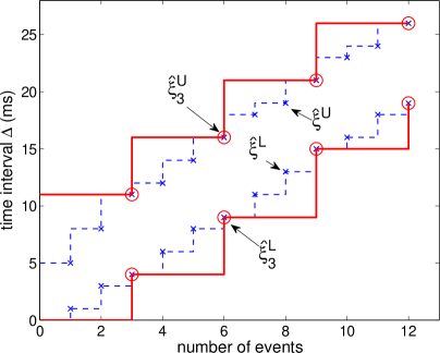
Figure 13: Example of fine and coarse input arrival curves $\hat{\xi}^{L/U}$ and $\hat{\xi}^{L/U}_{3}$

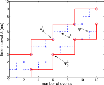
Figure 14: Example of fine and coarse service curves $\psi^{L/U}$ and $\psi^{L/U}_{3}$

A.2 Output Curves

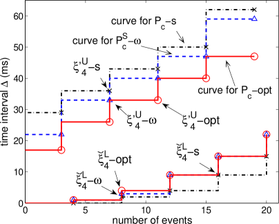
Figure 15: Comparison of output arrival curves at $g=4$ using simple coarse PMC $\mathcal{P}_{c}$, coarse PMC with $\omega$ $\mathcal{P}_{c}$-$\omega$ and optimized PMC $\mathcal{P}_{c}$-opt

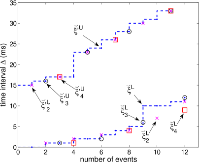
Figure 16: Comparison between fine and coarse output arrival curves computed from fine and optimized coarse PMC models respectively

A.3 Combined Output Curves

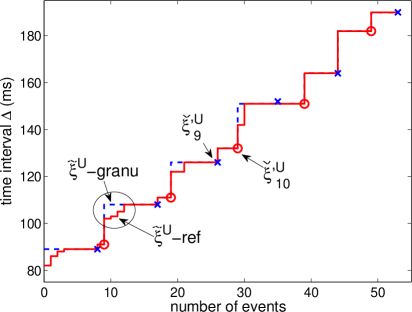
Figure 17: Computed fine upper output arrival curves $\tilde{\xi}^{U}$-granu (with simple scheme) and $\tilde{\xi}^{U}$-ref (with mathematical refinement algorithm)

References

- [1]
- [2] Karine Altisen & Matthieu Moy (2009): Connecting Real-Time Calculus to the Synchronous Programming Language Lustre. Technical Report TR-2009-14, Verimag.
- [3] Karine Altisen & Matthieu Moy (2010): Arrival Curves for Real-Time Calculus: the Causality Problem and its Solutions. In: TACAS.
- [4] R. Alur & D. L. Dill (1994): A theory of timed automata. Theoretical Computer Science 126, pp. 183–235.
- [5] G. Behrmann, K.G. Larsen & J.I. Rasmussen (2005): Optimal scheduling using priced timed automata. ACM SIGMETRICS Performance Evaluation Review 32(4), pp. 34–40.
- [6] Alessandro Bogliolo, Luca Benini, Emanuele Lattanzi & Giovanni De Micheli (2004): Specification and Analysis of Power-Managed Systems. Proceedings of the IEEE 92(8), pp. 1308–1346.
- [7] CATS tool. www.timestool.com/cats/.
- [8] S. Chakraborty, S. Künzli & L. Thiele (2003): A General Framework for Analysing System Properties in Platform-Based Embedded System Designs. In: DATE.
- [9] Samarjit Chakraborty, Thi Xuan Linh Phan & P.S. Thiagarajan (2005): Event Count Automata: A State-based Model for Stream Processing Systems. In: RTSS.
- [10] R. Henia, A. Hamann, M. Jersak, R. Racu, K. Richter & R. Ernst (2005): System level performance analysis - the SymTA/S approach. IEE Proc. Computers and Digital Techniques 152(2), pp. 148–166.
- [11] Simon Künzli, Arne Hamann, Rolf Ernst & Lothar Thiele (2007): Combined Approach to System Level Performance Analysis of Embedded Systems. In: CODES/ISSS.
- [12] Kai Lampka, Simon Perathoner & Lothar Thiele (2009): Analytic Real-Time Analysis and Timed Automata: A Hybrid Method for Analyzing Embedded Real-Time Systems. In: EMSOFT. AC.
- [13] Yanhong Liu, Karine Altisen & Matthieu Moy (2009): Granularity-based Interfacing between RTC and Timed Automata Performance Models. Technical Report TR-2009-10, Verimag.
- [14] Matthieu Moy & Karine Altisen (2009): Arrival Curves for Real-Time Calculus: the Causality Problem and its Solutions. Technical Report TR-2009-15, Verimag.
- [15] Simon Perathoner, Ernesto Wandeler & Lothar Thiele etc. (2007): Influence of Different System Abstractions on the Performance Analysis of Distributed Real-Time Systems. In: EMSOFT.
- [16] Linh T.X. Phan, S. Chakraborty & P. S. Thiagarajan (2008): A Multi-mode Real-Time Calculus. In: RTSS.
- [17] Linh T.X. Phan, Samarjit Chakraborty, P S Thiagarajan & Lothar Thiele (2007): Composing Functional and State-based Performance Models for Analyzing Heterogeneous Real-Time Systems. In: RTSS.
- [18] Simon Schliecker, Steffen Stein & Rolf Ernst (2007): Performance analysis of complex systems by integration of dataflow graphs and compositional performance analysis. In: DATE.
- [19] Lothar Thiele, Samarjit Chakraborty & Martin Naedele (2000): Real-time Calculus for Scheduling Hard Real-Time Systems. In: Int. Symp. on Circuits and Systems ISCAS, 4. pp. 101–104.