Spitzer spectroscopy of mass loss and dust production by evolved stars in globular clusters
Abstract
We have observed a sample of 35 long-period variables and four Cepheid variables in the vicinity of 23 Galactic globular clusters using the Infrared Spectrograph on the Spitzer Space Telescope. The long-period variables in the sample cover a range of metallicities from near solar to about 1/40th solar. The dust mass-loss rate from the stars increases with pulsation period and bolometric luminosity. Higher mass-loss rates are associated with greater contributions from silicate grains. The dust mass-loss rate also depends on metallicity. The dependence is most clear when segregating the sample by dust composition, less clear when segregating by bolometric magnitude, and absent when segregating by period. The spectra are rich in solid-state and molecular features. Emission from alumina dust is apparent across the range of metallicities. Spectra with a 13-m dust emission feature, as well as an associated feature at 20 m, also appear at most metallicities. Molecular features in the spectra include H2O bands at 6.4–6.8 m, seen in both emission and absorption, SO2 absorption at 7.3–7.5 m, and narrow emission bands from CO2 from 13.5 to 16.8 m. The star Lyngå 7 V1 has an infrared spectrum revealing it to be a carbon star, adding to the small number of carbon stars associated with Galactic globular clusters.
Subject headings:
globular clusters: general — stars: AGB and post-AGB — infrared: stars — circumstellar matter1. Introduction
Stars ascending the asymptotic giant branch (AGB) burn hydrogen and helium in shells around an inert C-O core (e.g., Iben & Renzini, 1983). The fusion of helium to carbon proceeds by the triple- sequence (Salpeter, 1952) in thermal pulses which lead to the dredge-up of freshly produced carbon to the surface of the star. If the envelope of the star is not too massive and the dredge-ups are sufficiently strong, then enough carbon reaches the surface to drive the photospheric C/O ratio over unity. Generally, the formation of CO molecules will exhaust whichever of the carbon or oxygen is less abundant, leading to a chemical dichotomy. Carbon stars produce carbon-rich dust, and oxygen-rich stars produce oxygen-rich dust. Stars in the range from 2–5 M⊙ become carbon stars, although both the lower and upper mass limits decrease in more metal-poor environments (e.g. Karakas & Lattanzio, 2007).
Several surveys with the Infrared Spectrograph (IRS; Houck et al., 2004) on the Spitzer Space Telescope (Werner et al., 2004) have probed how the production of dust by evolved stars depends on metallicity by observing AGB stars and supergiants in the Magallanic Clouds and other nearby Local Group galaxies. Carbon stars dominate these samples. The rate at which they produce dust does not vary significantly with metallicity (Groenewegen et al., 2007; Sloan et al., 2008, and references therein). It would appear that they produce and dredge up all of the carbon they need to form dust, regardless of their initial abundances (Sloan et al., 2009).
The published Local Group samples contain fewer oxygen-rich evolved stars, making any conclusions about this population more tentative. Sloan et al. (2008) compared oxygen-rich sources in the Galaxy, Large Magellanic Cloud (LMC), and Small Magellanic Cloud (SMC), and they found that as the metallicity of the sample decreased, the fraction of stars with a dust excess decreased. Infrared photometric surveys of several dwarf irregular galaxies in the Local Group also show a trend of less dust at lower metallicities (Boyer et al., 2009a).
The spectroscopic evidence for a dependency of dust production on metallicity is not strong. Stars in the Magellanic Clouds can pulsate with periods of 700 days or longer, and these longer-period variables are usually embedded in significant amounts of dust, with no apparent dependence on metallicity. Additional oxygen-rich sources from the SMC further blur the trends noticed before (Sloan et al., 2010). One major problem with these samples is that oxygen-rich evolved stars can come from three distinct populations. The red supergiants and intermediate-mass AGB stars (or super-AGB stars) are too massive to become carbon stars, while the low-mass AGB stars have too little mass. This mixing of populations confuses the observed samples of oxygen-rich evolved stars in the Galaxy, the Magellanic Clouds, and more distant irregulars in the Local Group.
Globular clusters provide another means of investigating dependencies of dust production on metallicity. Like the Magellanic Clouds, most globular clusters have known metallicities, and they are at known distances, allowing us to directly determine their luminosities. Unlike the Magellanic Clouds, globular clusters have old populations of stars, with few significantly younger than 10 billion years. This limits the sample to masses of 1M⊙ or less, below the lower mass limit for carbon stars.
Lebzelter et al. (2006) identified and observed 11 long-period variables (LPVs) in the globular cluster 47 Tuc with the IRS on Spitzer. Their data were consistent with a shift from relatively dust-free AGB stars to more deeply embedded sources with higher mass-loss rates at a luminosity of 2000 L☉. But with a sample of only one globular cluster, they were unable to address the important question of how the dust properties depend on metallicity.
We have used the IRS on Spitzer to observe a sample of 39 variable stars in 23 globular clusters spanning a range of metallicity from nearly solar to only a few percent of solar. This paper presents an overview of the program. § 2 describes the sample of clusters and individual stars and the observations, including near-infrared photometric monitoring prior to the Spitzer observations, the IRS spectroscopy, and nearly simultaneous near-infrared photometry. § 3 assesses the membership of our targets within the clusters, while § 4 describes the analysis and the results. § 5 treats some unusual objects individually, and § 6 examines the larger picture of evolution on the AGB.
2. Observations
| Globular | Alternative | Distance | |||||
|---|---|---|---|---|---|---|---|
| Cluster | Name | [Fe/H] | Ref. aaReferences: (1) Harris (2003); (2) Carretta & Gratton (1997); (3) Ferraro et al. (1999); (4) Recio-Blanco et al. (2005); (5) Carretta et al. (2009); (6) Dotter et al. (2010); (7) Carretta et al. (2000); (8) Gratton et al. (1997); (9) Morgan & Dickerson (2000) ; (10) McNamara (2000); (11) Thompson et al. (2001); (12) Kaluzny et al. (2002); (13) Caputo et al. (2002); (14) Del Principe et al. (2006); (15) Catelan (2006); (16) van de Ven et al. (2006); (17) Salaris & Weiss (1998); (18) Sarajedini (2004); (19) Carretta et al. (2007); (20) Dalessandro et al. (2008); (21) Matsunaga (2007b); (22) See § 2.1; (23) Barbuy et al. (1998a); (24) Ortolani et al. (1998); (25) Lee & Carney (2002); (26) Origlia & Rich (2004); (27) Valenti et al. (2007); (28) This work (§ 3.1); (29) Valenti et al. (2004); (30) Heitsch & Richtler (1999); (31) Matsunaga et al. (2009); (32) Barbuy et al. (1998b); (33) Valenti et al. (2005); (34) Ivanov et al. (2000); (35) Kaisler et al. (1997). | E(BV) | Ref. aaReferences: (1) Harris (2003); (2) Carretta & Gratton (1997); (3) Ferraro et al. (1999); (4) Recio-Blanco et al. (2005); (5) Carretta et al. (2009); (6) Dotter et al. (2010); (7) Carretta et al. (2000); (8) Gratton et al. (1997); (9) Morgan & Dickerson (2000) ; (10) McNamara (2000); (11) Thompson et al. (2001); (12) Kaluzny et al. (2002); (13) Caputo et al. (2002); (14) Del Principe et al. (2006); (15) Catelan (2006); (16) van de Ven et al. (2006); (17) Salaris & Weiss (1998); (18) Sarajedini (2004); (19) Carretta et al. (2007); (20) Dalessandro et al. (2008); (21) Matsunaga (2007b); (22) See § 2.1; (23) Barbuy et al. (1998a); (24) Ortolani et al. (1998); (25) Lee & Carney (2002); (26) Origlia & Rich (2004); (27) Valenti et al. (2007); (28) This work (§ 3.1); (29) Valenti et al. (2004); (30) Heitsch & Richtler (1999); (31) Matsunaga et al. (2009); (32) Barbuy et al. (1998b); (33) Valenti et al. (2005); (34) Ivanov et al. (2000); (35) Kaisler et al. (1997). | Modulus | Ref. aaReferences: (1) Harris (2003); (2) Carretta & Gratton (1997); (3) Ferraro et al. (1999); (4) Recio-Blanco et al. (2005); (5) Carretta et al. (2009); (6) Dotter et al. (2010); (7) Carretta et al. (2000); (8) Gratton et al. (1997); (9) Morgan & Dickerson (2000) ; (10) McNamara (2000); (11) Thompson et al. (2001); (12) Kaluzny et al. (2002); (13) Caputo et al. (2002); (14) Del Principe et al. (2006); (15) Catelan (2006); (16) van de Ven et al. (2006); (17) Salaris & Weiss (1998); (18) Sarajedini (2004); (19) Carretta et al. (2007); (20) Dalessandro et al. (2008); (21) Matsunaga (2007b); (22) See § 2.1; (23) Barbuy et al. (1998a); (24) Ortolani et al. (1998); (25) Lee & Carney (2002); (26) Origlia & Rich (2004); (27) Valenti et al. (2007); (28) This work (§ 3.1); (29) Valenti et al. (2004); (30) Heitsch & Richtler (1999); (31) Matsunaga et al. (2009); (32) Barbuy et al. (1998b); (33) Valenti et al. (2005); (34) Ivanov et al. (2000); (35) Kaisler et al. (1997). |
| NGC 362 | 1.20 | 1,2,3,4,5,6 | 0.04 0.02 | 1,3,4,7 | 14.83 0.15 | 1,3,4,6,7,8 | |
| NGC 5139 | Cen | 1.63 | 1,5 | 0.12 0.01bbUncertainty assumed. | 1 | 13.70 0.17 | 1,9,10,11,12,13,14,15,16 |
| NGC 5904 | M 5 | 1.20 | 2,3,4,5,6 | 0.03 0.01 | 1,3,4,7,17 | 14.46 0.10 | 1,3,4,6,7,8,17 |
| NGC 5927 | 0.35 | 1,3,4,5,6 | 0.46 0.05bbUncertainty assumed. | 1,3 | 14.45 0.07 | 1,3,4,6 | |
| Lyngå 7 | 0.66 | 1,6,18 | 0.73 0.12 | 1,18 | 14.31 0.10 | 1,18 | |
| NGC 6171 | M 107 | 0.98 | 1,3,4,5,6 | 0.38 0.08 | 1,3,4,17 | 13.89 0.18 | 1,3,4,17 |
| NGC 6254 | M 10 | 1.51 | 1,3,5,6 | 0.28 0.03bbUncertainty assumed. | 1,3 | 13.30 0.12 | 1,3 |
| NGC 6352 | 0.69 | 1,3,5,6 | 0.21 0.02bbUncertainty assumed. | 1,3 | 13.85 0.06 | 1,3,17 | |
| NGC 6356 | 0.50 | 1,4,5 | 0.28 0.03bbUncertainty assumed. | 1 | 15.93 0.09 | 1,4 | |
| NGC 6388 | 0.57 | 1,4,5,19 | 0.35 0.04 | 1,20 | 15.47 0.12 | 4,20,21 | |
| Palomar 6 | 22 | 1.36 0.14bbUncertainty assumed. | 1,23,24,25 | 14.23 0.40 | 1,23,24,25 | ||
| Terzan 5 | 0.08 | 1,5,23,26,27 | 2.31 0.23bbUncertainty assumed. | 1,23,27 | 14.11 0.13 | 28 | |
| NGC 6441 | 0.56 | 1,4,5,29 | 0.50 0.05bbUncertainty assumed. | 1,29 | 15.57 0.16 | 1,4,29,30,31 | |
| NGC 6553 | 0.28 | 1,3,5 | 0.72 0.11 | 1,3,23 | 13.63 0.22 | 1,3,23,30 | |
| IC 1276 | Palomar 7 | 0.69 | 1,5 | 1.12 0.11bbUncertainty assumed. | 1,32 | 13.66 0.15bbUncertainty assumed. | 1 |
| Terzan 12 | 0.50 | 23 | 2.06 0.21bbUncertainty assumed. | 23 | 13.38 0.15bbUncertainty assumed. | 1 | |
| NGC 6626 | M 28 | 1.46 | 1,5 | 0.40 0.04bbUncertainty assumed. | 1 | 13.73 0.15bbUncertainty assumed. | 1 |
| NGC 6637 | M 69 | 0.66 | 1,3,4,5,6,33 | 0.16 0.02 | 1,3,33 | 14.76 0.09 | 1,3,4,21,33 |
| NGC 6712 | 0.97 | 1,3,5 | 0.43 0.04 | 1,3,4 | 14.24 0.09 | 1,3,4 | |
| NGC 6760 | 0.48 | 1,4,5 | 0.77 0.08bbUncertainty assumed. | 1 | 14.59 0.29 | 1,4 | |
| NGC 6779 | M 56 | 2.05 | 1,5,6 | 0.19 0.08 | 1,34 | 15.23 0.30 | 1,34 |
| Palomar 10 | 0.10 | 1 | 1.66 0.17bbUncertainty assumed. | 1,31 | 13.86 0.37 | 1,32 | |
| NGC 6838 | M 71 | 0.73 | 1,2,3,4,5,6 | 0.26 0.03bbUncertainty assumed. | 1,2,3 | 12.99 0.10 | 1,3,4,7 |
| RA | Dec. | IRS observations | Var. | Period | Mean magnitudes | Phase | |||||||
|---|---|---|---|---|---|---|---|---|---|---|---|---|---|
| Target | J2000 | AOR key | Date (JD) | ClassaaSR = semi-regular; CW = Cepheid of the W Vir type (i.e. Pop. II). | (days) | J | H | K | Ks | Zero (JD) | Obs.bbPhase during the IRS observation for P 50 days. | Notes | |
| NGC 362 V2 | 01 03 21.85 | 70 54 20.1 | 21740800 | 2454268 | SR | 89.0 | 9.74 | 9.11 | 8.93 | 0.18 | 2452445.7 | 0.48 | |
| NGC 362 V16 | 01 03 15.10 | 70 50 32.3 | 21740800 | 2454268 | Mira/SR | 138 | 9.09 | 8.41 | 8.18 | 0.52 | 2452495.5 | 0.81 | |
| NGC 5139 V42 | 13 26 46.36 | 47 29 30.4 | 21741056 | 2454310 | Mira | 149 | 8.25 | 7.52 | 7.14 | 0.52 | 2452525.7 | 0.97 | |
| NGC 5904 V84 | 15 18 36.15 | 02 04 16.3 | 21741312 | 2454316 | CW | 25.8 | 10.05 | 9.67 | 9.60 | 0.69 | 2452400.5 | ||
| NGC 5927 V1 | 15 28 15.17 | 50 38 09.3 | 21741568 | 2454348 | Mira/SR | 202 | 9.17 | 8.27 | 7.87 | 0.38 | 2452475.6 | 0.29 | |
| NGC 5927 V3 | 15 28 00.13 | 50 40 24.6 | 21741824 | 2454348 | Mira | 297 | 8.72 | 7.84 | 7.33 | 0.89 | 2452582.5 | 0.94 | |
| Lyngå 7 V1 | 16 11 02.05 | 55 19 13.5 | 21742080 | 2454350 | Mira | 551 | 11.35 | 9.08 | 7.25 | 1.22 | 2452856.2 | 0.71 | |
| NGC 6171 V1 | 16 32 24.61 | 13 12 01.3 | 21742336 | 2454345 | Mira | 332 | 6.02 | 5.16 | 4.54 | c | |||
| NGC 6254 V2 | 16 57 11.74 | 04 03 59.7 | 21742592 | 2454347 | CW | 19.7 | 10.12 | 9.59 | 9.44 | 0.71 | 2452394.4 | ||
| NGC 6352 V5 | 17 25 37.52 | 48 22 10.0 | 21742848 | 2454384 | Mira | 177 | 8.34 | 7.43 | 7.07 | 0.32 | 2452492.7 | 0.66 | |
| NGC 6356 V1 | 17 23 33.72 | 17 49 14.8 | 21743104 | 2454375 | Mira | 227 | 10.18 | 9.29 | 8.83 | 0.61 | 2452525.5 | 0.15 | |
| NGC 6356 V3 | 17 23 33.30 | 17 48 07.4 | 21743104 | 2454375 | Mira | 223 | 10.18 | 9.37 | 8.93 | 0.80 | 2452548.8 | 0.21 | |
| NGC 6356 V4 | 17 23 48.00 | 17 48 04.5 | 21743104 | 2454375 | Mira | 211 | 10.33 | 9.47 | 9.05 | 0.66 | 2452546.6 | 0.68 | |
| NGC 6356 V5 | 17 23 17.06 | 17 46 24.5 | 21743104 | 2454375 | Mira | 220 | 9.33 | 9.06 | 8.62 | c | |||
| NGC 6388 V3 | 17 36 15.04 | 44 43 32.5 | 21743360 | 2454377 | Mira | 156 | 10.29 | 9.25 | 8.97 | 0.28 | 2452345.7 | 0.99 | |
| NGC 6388 V4 | 17 35 58.94 | 44 43 39.8 | 21743360 | 2454377 | Mira | 253 | 9.64 | 8.89 | 8.47 | 0.80 | 2452437.7 | 0.66 | |
| Palomar 6 V1 | 17 43 49.48 | 26 15 27.9 | 21743616 | 2454374 | Mira | 566 | 11.65 | 8.82 | 1.53 | 2452653.9 | 0.04 | ||
| Terzan 5 V2 | 17 47 59.46 | 24 47 17.6 | 21743872 | 2454374 | Mira | 217 | 9.78 | 8.38 | 7.65 | 0.67 | 2452464.4 | 0.80 | |
| Terzan 5 V5 | 17 48 03.40 | 24 46 42.0 | 21744128 | 2454374 | Mira | 464 | 10.03 | 8.04 | 6.83 | 0.86 | 2452557.9 | 0.91 | |
| Terzan 5 V6 | 17 48 09.25 | 24 47 06.3 | 21744128 | 2454374 | Mira | 269 | 10.01 | 8.41 | 7.50 | 0.61 | 2452366.0 | 0.47 | |
| Terzan 5 V7 | 17 47 54.33 | 24 49 54.6 | 21744128 | 2454374 | Mira | 377 | 9.74 | 8.02 | 7.03 | 0.76 | 2452511.8 | 0.95 | |
| Terzan 5 V8 | 17 48 07.18 | 24 46 26.6 | 21744128 | 2454374 | Mira | 261 | 9.79 | 8.28 | 7.44 | 0.80 | 2452459.2 | 0.35 | |
| Terzan 5 V9 | 17 48 11.86 | 24 50 17.1 | 21743872 | 2454374 | Mira | 464 | 11.43 | 9.55 | 8.41 | 0.83 | 2452401.0 | 0.25 | |
| NGC 6441 V1 | 17 50 17.09 | 37 03 49.7 | 21744384 | 2454577 | Mira | 200 | 10.28 | 9.26 | 8.90 | 0.40 | 2452495.1 | 0.40 | |
| NGC 6441 V2 | 17 50 16.16 | 37 02 40.5 | 21744384 | 2454577 | Mira | 145 | 10.50 | 9.57 | 9.23 | 0.52 | 2452372.0 | 0.18 | |
| NGC 6553 V4 | 18 09 18.84 | 25 54 35.8 | 21744640 | 2454373 | Mira | 267 | 8.17 | 7.21 | 6.66 | 1.06 | 2452727.2 | 0.16 | |
| IC 1276 V1 | 18 10 51.55 | 07 10 54.5 | 21742080 | 2454376 | Mira | 222 | 8.43 | 7.31 | 6.77 | 0.29 | 2452511.4 | 0.41 | |
| IC 1276 V3 | 18 10 50.79 | 07 13 49.1 | 21742080 | 2454376 | Mira | 300 | 8.27 | 7.25 | 6.60 | 0.89 | 2452422.2 | 0.51 | |
| Terzan 12 V1 | 18 12 14.18 | 22 43 58.9 | 21745152 | 2454373 | Mira | 458 | 8.87 | 7.21 | 6.23 | 1.02 | 2452586.6 | 0.90 | |
| NGC 6626 V17 | 18 24 35.84 | 24 53 15.8 | 21745408 | 2454375 | CW | 48.6 | 9.38 | 8.76 | 8.61 | 0.51 | 2452405.2 | ||
| NGC 6637 V4 | 18 31 21.88 | 32 22 27.7 | 21745664 | 2454582 | Mira | 200 | 8.97 | 8.26 | 7.86 | 0.58 | 2452378.1 | 0.00 | |
| NGC 6637 V5 | 18 31 23.44 | 32 20 49.5 | 21745664 | 2454582 | Mira | 198 | 8.94 | 8.21 | 7.82 | 0.73 | 2452376.1 | 0.16 | |
| NGC 6712 V2 | 18 53 08.78 | 08 41 56.6 | 21745920 | 2454385 | SR | 109 | 9.11 | 8.45 | 8.16 | 0.54 | 2452446.2 | 0.86 | |
| NGC 6712 V7 | 18 52 55.38 | 08 42 32.5 | 21745920 | 2454385 | Mira | 193 | 8.69 | 7.95 | 7.55 | 0.55 | 2452525.4 | 0.64 | |
| NGC 6760 V3 | 19 11 14.31 | 01 01 46.6 | 21746176 | 2454381 | Mira | 251 | 9.12 | 8.24 | 7.69 | 0.72 | 2452417.7 | 0.82 | |
| NGC 6760 V4 | 19 11 15.03 | 01 02 36.8 | 21746432 | 2454381 | Mira | 226 | 9.39 | 8.55 | 7.96 | 0.94 | 2452486.6 | 0.40 | |
| NGC 6779 V6 | 19 16 35.78 | 30 11 38.8 | 21746688 | 2454269 | CW | 44.9 | 10.68 | 10.23 | 10.09 | 0.66 | 2453214.4 | ||
| Palomar 10 V2 | 19 17 51.48 | 18 34 12.7 | 21746944 | 2454269 | Mira | 393 | 6.79 | 5.58 | 4.87 | c | |||
| NGC 6838 V1 | 19 53 56.10 | 18 47 16.8 | 21746944 | 2454269 | Mira/SR | 179 | 7.59 | 6.85 | 6.57 | 0.32 | 2452421.6 | 0.34 | |
2.1. The Clusters
Table 1 presents the metallicity, reddening, and distance modulus to the clusters in our sample. The values for each are based on a review of the literature, starting with the catalog of Harris (2003), which was published in 1996 and updated on the web in 2003. Most of the estimates for metallicity and reddening are unchanged between the two editions for our target clusters, but most of the distances have changed, usually by small amounts. We have also included measurements of the metallicity and distance modulus published since 1996, taking care not to overweight references included in the 2003 updates to the bibliography of the catalog. We have averaged the measurements for metallicity, reddening, and distance modulus. For the latter two, we also quote the standard deviation as the uncertainty, which propagates through the quantities we derive. We take the minimum uncertainty for to be 10% of the mean. In some cases, we have quoted the uncertainties given by the referenced papers. Some data which vary substantially from the others have been excluded (and are not included in the references in Table 1).
For IC 1276 and Terzan 12, we excluded distance modulus measurements inconsistent with our estimates based on the period-K relation (§ 3.1). For Terzan 5, we report the distance modulus based on the analysis of the four relatively unreddened variables in our sample (§ 3.1).
The metallicity of Palomar 6 is problematic, with measurements in the refereed literature ranging from 1.08 (Lee & Carney, 2002) to +0.2 (Minniti, 1995). Intermediate measurements of 0.74 (Zinn, 1985) and 0.52 (Stephens & Frogel, 2004) have also been reported. Averaging these metallicities gives [Fe/H] = 0.540.54. With a standard deviation as large as the mean, we are unable to determine a metallicity for this cluster with any confidence.
The metallicity of the cluster is important, because we assign individual stars to bins based on their metallicity. Each bin will contain between five and eight targets, all with a similar metallicity. By comparing how the properties of the stars vary from one bin to the next, we can assess how the mass-loss and dust production depend on metallicity.
2.2. Photometric Monitoring and Sample Selection

We selected the variable stars in the sample based on JHK photometry from the South African Astronomical Observatory (SAAO). Observations were made using the SIRIUS near-infrared camera (Simultaneous-Color Infrared Imager for Unbiased Surveys; Nagayama et al., 2003) at the 1.4-m Infrared Survey Facility (IRSF) telescope over the period from 2002 to 2005. The IRSF/SIRIUS survey imaged fields in the vicinity of globular clusters at J, H, and Ks (central wavelengths of 1.25, 1.63, and 2.14 m) with a typical sampling interval of 40–60 days (Matsunaga, 2007a).
The field of view of the survey was 7.7 arcmin2, and most clusters were imaged out to the half-mass radius. Many new variables were discovered, including eight new long-period variables: Lyngå 7 V1, Palomar 6 V1, Terzan 5 V5–V9, and Terzan 12 V1. All eight of these stars are Miras, and their periods range from 260 to 570 days. The remaining 31 targets in our sample were previously known variables (Clement et al., 2001, and references therein).
We determined periods, mean magnitudes, amplitudes and phases for each variable by performing Fourier analysis and minimum- fits to the individual photometric observations in each SIRIUS filter for each target. The results appear in Table 2 and Figure 1. The quoted period and phase are the average from the three filters, except in cases where one filter disagreed substantially from the other two, or for Palomar 6 V1, which was too reddened for measurements at J. Generally, the uncertainty in the period was less than one day.111In three cases, Lyngå 7 V1, Terzan 5 V9, and NGC 6838 V1, it was larger, 5–6 days. We lack monitoring observations of NGC 6171 V1, NGC 6356 V5, and Palomar 10 V2. For these sources, Table 2 contains variability information from Clement et al. (2001) and photometry from 2MASS (Skrutskie et al., 2006).
The four “CW” variables are Pop. II Cepheids (of the W Vir type). They all have periods which are very short compared to the monitoring period, so any irregularities in the pulsations can accumulate to smear out the apparent periodicity in Figure 1. Furthermore, we are unable to reproduce the published periods for NGC 6626 V17 and NGC 6779 V6, which are 92.1 and 90 days, respectively (Clement et al., 2001). Instead, we find a period of 48.6 days for NGC 6626 V17 and 44.9 days for NGC 6779 V6. These appear to be overtones of the previously published periods, but we cannot say whether that is the result of an actual mode-shift in pulsation or sampling resolution of the older data.
2.3. IRS Spectroscopy


We observed the sample of variables in Table 2 with the IRS on Spitzer, using the Short-Low (SL) module on all targets and the Long-Low (LL) module on all but the three faintest. The data reduction began with the flatfielded images produced by the S18 version of the data pipeline from the Spitzer Science Center (SSC). To subtract the background from these images, we generally used images with the source in the other aperture in SL (aperture differences) and images with the source in the other nod position in the same aperture in LL (nod differences). In crowded fields, we occasionally had to resort to whichever background image resulted in the least confusion. We then corrected the bad pixels in the differenced images using the imclean IDL package222Available from the SSC as irsclean.. Bad pixels included those flagged in the bit-mask images accompanying the data images and those flagged as rogues in the campaign rogue masks provided by the SSC. We stacked the campaign rogue masks to produce super-rogue masks, considering a pixel to be bad if it had been identified as such in any two previous campaign rogue masks.
We used two methods to extract spectra from the corrected images. The older method uses the profile, ridge, and extract routines available in the SSC’s Spitzer IRS Custom Extractor (SPICE). This method produces the equivalent of a tapered-column extraction in SMART (Higdon et al., 2004)333SMART is the Spectroscopic Modeling, Analysis, and Reduction Tool., summing the flux within an aperture which increases in width proportionally with wavelength. It is the basis for the spectra in most of the IRS papers referenced in the introduction. This globular cluster data-set is one of the first to make use of the optimal extraction algorithm available in the new release of SMART (Lebouteiller et al., 2010). This algorithm fits a super-sampled point-spread function (PSF) to the data, improving the signal/noise (S/N) ratio of the data by a factor of 1.8, typically. Optimal extraction also allows the extraction of sources with overlapping PSFs, which is particularly useful in the crowded regions typical for globular clusters.
We used the optimal extraction for all of our data except for the LL portion of three targets: NGC 362 V16, Terzan 5 V5, and NGC 6441 V2. In these cases, the optimal algorithm was unable to separate our intended target from adjacent sources, and for these, we used the tapered-column extraction.
The calibration of SL spectra is based on observations of HR 6348 (K0 III). The calibration of LL used HR 6348 along with the late K giants HD 166780 and HD 173511. We extracted the spectra of these stars using the optimal and tapered-column algorithms to calibrate the two extraction methods independently.
The final step in the data reduction corrects for discontinuities between the orders and trims untrustworthy data from the ends of each order. The correction for discontinuities applies scalar multiplicative adjustments to each order, shifting them upwards to the presumably best-centered segment. The exception is the three targets blended with other sources in LL. For these, we normalized to SL1 to minimize the impact on our measured bolometric magnitudes of the contamination from the additional sources in LL.
Figures 2 through 8 present the resulting spectra for the targets in Table 2, organized by the metallicity of the clusters of which they are members (and ordered by the right ascension of the cluster). Figure 7 includes the four Cepheids, three of which were observed with SL only, and Figure 8 includes those sources which are not oxygen-rich (Lyngå 7 V1), are members of clusters with highly uncertain metallicities (Palomar 6 V1), or whose membership or evolutionary status is uncertain (§ 3.4).
2.4. Contemporaneous Photometry
| Target | J | H | K | L | JD |
|---|---|---|---|---|---|
| NGC 362 V16 | 9.384 0.011 | 8.671 0.007 | 8.469 0.006 | 8.046 0.036 | 2454376 |
| NGC 362 V2 | 9.781 0.011 | 9.017 0.007 | 8.829 0.005 | 8.571 0.056 | 2454376 |
| NGC 5139 V42 | 8.694 0.011 | 7.908 0.037 | 7.583 0.032 | 6.974 0.022 | 2454376 |
| NGC 5904 V84 | 9.931 0.008 | 9.587 0.009 | 9.525 0.008 | 9.308 0.115 | 2454376 |
| NGC 5927 V1 | 9.422 0.013 | 8.379 0.005 | 7.961 0.004 | 7.387 0.049 | 2454376 |
| NGC 5927 V3 | 8.309 0.011 | 7.289 0.006 | 6.869 0.006 | 6.238 0.018 | 2454376 |
| Lyngå 7 V1 | 11.653 0.021 | 9.308 0.019 | 7.317 0.009 | 4.896 0.017 | 2454376 |
| NGC 6171 V1 | 5.842 0.007 | 5.069 0.040 | 4.623 0.010 | 3.772 0.018 | 2454376 |
| NGC 6254 V2 | 9.749 0.018 | 9.322 0.017 | 9.231 0.017 | 9.004 0.099 | 2454376 |
| NGC 6356 V1 | 9.986 0.015 | 9.136 0.010 | 8.674 0.006 | 8.063 0.038 | 2454375 |
| NGC 6356 V3 | 10.490 0.029 | 9.619 0.015 | 9.151 0.008 | 8.649 0.067 | 2454375 |
| NGC 6356 V4 | 10.352 0.022 | 9.458 0.014 | 9.118 0.007 | 8.683 0.079 | 2454375 |
| NGC 6356 V5 | 10.030 0.019 | 9.113 0.016 | 8.777 0.005 | 8.231 0.048 | 2454375 |
| NGC 6388 V3 | 10.303 0.025 | 9.203 0.026 | 8.957 0.013 | 8.602 0.064 | 2454376 |
| NGC 6388 V4 | 9.781 0.007 | 8.926 0.005 | 8.563 0.017 | 7.925 0.039 | 2454376 |
| Palomar 6 V1 | 14.010 0.078 | 10.508 0.029 | 8.036 0.019 | 5.471 0.030 | 2454376 |
| Terzan 5 V2 | 9.980 0.013 | 8.515 0.008 | 7.802 0.006 | 6.947 0.021 | 2454376 |
| Terzan 5 V5 | 9.413 0.011 | 7.496 0.007 | 6.511 0.005 | 5.472 0.016 | 2454376 |
| Terzan 5 V6 | 10.323 0.028 | 8.609 0.013 | 7.724 0.017 | 6.712 0.021 | 2454376 |
| Terzan 5 V7 | 9.369 0.007 | 7.763 0.007 | 6.838 0.004 | 5.724 0.016 | 2454376 |
| Terzan 5 V8 | 9.764 0.032 | 8.257 0.029 | 7.467 0.008 | 6.589 0.018 | 2454376 |
| Terzan 5 V9 | 11.307 0.013 | 9.301 0.009 | 8.173 0.007 | 7.006 0.029 | 2454376 |
| NGC 6553 V4 | 7.905 0.020 | 6.735 0.014 | 6.298 0.015 | 5.787 0.038 | 2454375 |
| IC 1276 V1 | 8.604 0.013 | 7.417 0.008 | 6.882 0.005 | 6.283 0.017 | 2454375 |
| IC 1276 V3 | 8.926 0.013 | 7.786 0.009 | 7.015 0.010 | 6.083 0.048 | 2454375 |
| Terzan 12 V1 | 8.677 0.021 | 7.096 0.024 | 6.207 0.015 | 5.164 0.017 | 2454375 |
| NGC 6626 V17 | 9.133 0.024 | 8.585 0.018 | 8.394 0.033 | 8.271 0.044 | 2454375 |
| NGC 6760 V3 | 8.918 0.006 | 7.898 0.009 | 7.457 0.004 | 6.869 0.039 | 2454376 |
| NGC 6760 V4 | 9.779 0.008 | 8.739 0.006 | 8.142 0.004 | 7.356 0.023 | 2454376 |
| Palomar 10 V2 | 7.227 0.006 | 5.984 0.008 | 5.292 0.005 | 4.439 0.021 | 2454376 |
| NGC 6838 V1 | 7.449 0.006 | 6.597 0.005 | 6.283 0.004 | 5.830 0.016 | 2454376 |
Table 3 presents photometry of 31 of our 39 targets obtained from the 2.3-m telescope at Siding Spring Observatory (SSO) during the period when the Spitzer spectra were obtained. All observations were made using the Cryogenic Array Spectrometer/Imager (CASPIR; McGregor et al., 1994) with the following filters: J (effective wavelength 1.24 m), H (1.68 m), K (2.22 m), and narrow-band L (3.59 m). Calibrations were based on observations of standard stars from the lists of McGregor (1994), and the data were processed using standard tools available with IRAF (the Image Reduction and Analysis Facility).
3. Membership
The principal objective of this study is to investigate how the quantity and composition of the dust produced by AGB stars depend on its initial metallicity. We assume that the metallicity of a star is simply the metallicity of its cluster, making it important to identify non-members which are in the foreground or the background of a cluster. Our primary tools for testing membership are whether the relation between period and absolute K magnitude and the bolometric magnitude of the stars produces a distance consistent with membership, and if that distance results in a bolometric magnitude consistent with the masses of stars as old as those in our sample.
3.1. The Period-K Relation
We estimated the distance to each variable by applying the period-K magnitude relation of Whitelock et al. (2008). In general, = (log 2.38) + . Whitelock et al. (2008) found that = 3.51 in Mira variables in the LMC and the Galaxy, but varied from 7.15 in the LMC to 7.25 in the Galaxy. Whitelock et al. (2008) assumed that the distance modulus to the LMC was 18.39. The value for would be 7.25 for both the Galactic and LMC samples if the distance modulus to the LMC were 18.49, which compares favorably to recent measurements. Alves (2004) estimated the distance modulus to the LMC to be 18.500.02, based on a review of 14 recent determinations, and Keller & Wood (2006) found a value of 18.540.02, based on an analysis of bump Cepheids. Thus, we assume that =7.25 for all sources in the following analysis.
We dereddened the K magnitude using the estimates for given in Table 1 and the interstellar extinction measurements by Rieke & Lebofsky (1985), who find that and 444We will also use the ratios , , and elsewhere in this paper. We excluded the four Cepheid variables in our sample from this analysis, which accounts for all of the periods less than 50 days.
The period-K relation produces distance moduli for IC 1276 V1 and V3 of 13.51 and 13.81, respectively, while Harris (2003) reports 13.66 and Barbuy et al. (1998b) report 13.01. The latter is inconsistent with our estimates, and we adopt the former. Similarly, the period-K relation gives a distance modulus for Terzan 12 V1 of 13.75, compared to 13.38 (Harris, 2003) and 12.66 (Ortolani et al., 1998). This source has a period of 458 days, and we might expect circumstellar extinction at K of a few tenths of a magnitude. Thus we drop 12.66 as inconsistent with the period of the star and adopt 13.38 as the distance modulus.
Five of the six variables in Terzan 5 have an average distance modulus of 14.11 (0.13), compared to values of 15.05 (Harris, 2003), 13.87 (Valenti et al., 2007), and 13.70 (Ortolani et al., 2007). Terzan 5 V9 is heavily reddened at K, giving an apparent distance modulus of 15.86, widely at variance with the others. Differential reddening in front of Terzan 5 would have to produce 15.6 additional magnitudes of visual extinction and is an unlikely explanation. Ferraro et al. (2009) have identified a younger and more metal-rich population in Terzan 5 (age 6 Gyr and [Fe/H]+0.3). They present isochrones showing that the younger population should have roughly one extra magnitude of reddening in VK, but their isochrones are based on models which do not extend to the tip of the AGB. We cannot rule out the possibility that Terzan 5 V9 is a member of this younger population, but it clearly differs from the remaining sources in the cluster and to be cautious, we will treat it as a non-member. The distance moduli of the remaining five variables are mutually consistent with each other and nearly two standard deviations from the closest published estimate, 13.87. For the remainder of this paper, we will adopt our own mean distance modulus for Terzan 5: 14.11.
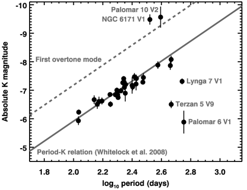
Figure 9 presents the period-K relation for our sample of globular cluster variables (excluding the Cepheids). The absolute K magnitudes are based on the distance moduli presented in Table 1. The labelled sources in the figure require special consideration, which in some cases has led to their exclusion as members. In Figure 9, though, their absolute magnitude is determined as though they were members. The figure also shows the period-K relation for fundamental-mode pulsators and for overtone pulsators, assuming that their periods are 2.3 times smaller.
Two sources appear to be too bright for the period-K relation: NGC 6171 V1 and Palomar 10 V2. While it is possible that they are overtone pulsators, their bolometric magnitudes are inconsistent with membership, as explained in the next section. Assuming that both are fundamental-mode pulsators, NGC 6171 V1 has a distance modulus of 12.15, compared to 13.89 for the cluster, putting it 3.3 kpc in front of the cluster and 1.1 kpc above the Galactic plane. Similarly, Palomar 10 V2 has a distance modulus of 12.30 vs. 13.86 for the cluster, which means it is 3.0 kpc closer and about 0.14 kpc above the Galactic plane.
The three sources below the period-K relation present more complex cases. We will examine them after determining bolometric magnitudes (next section).
3.2. Bolometric Magnitudes
| log | Corrected | IR Spec. | |||||
|---|---|---|---|---|---|---|---|
| Target | [7][15] | DECaaDust emission contrast; see §4.1 for an explanation and a discussion of systematic errors. | (M☉ /yr)bbSubtract 2.30 to convert to log10 of the dust-production rate (see §4.2). | ClassccPhotometry from 2MASS, variability class and period from Clement et al. (2001). | Notes | ||
| NGC 362 V2 | 3.50 | 0.46 0.02 | 0.09 0.01 | 7.90 0.06 | 1.N | ||
| NGC 362 V16 | 4.10 | 0.25 0.02 | 0.02 0.00 | 8.54 0.44 | 1.N | ||
| NGC 5139 V42 | 3.88 | 0.41 0.01 | 0.07 0.00 | 8.02 0.11 | 1.N | ||
| NGC 5904 V84 | 3.05 | 0.06 0.03 | 1.N | d, e | |||
| NGC 5927 V1 | 4.13 | 1.19 0.02 | 0.67 0.01 | 6.65 0.11 | 1.22 0.01 | 2.SX4t | |
| NGC 5927 V3 | 4.64 | 1.35 0.00 | 1.48 0.00 | 6.27 0.03 | 1.57 0.05 | 2.SE8t | |
| Lyngå 7 V1 | 4.99 | 0.58 0.01 | 6.61 0.01 | 2.CE | |||
| NGC 6171 V1 | 5.11 | 1.53 0.01 | 1.99 0.01 | 6.02 0.07 | 1.68 0.06 | 2.SE8 | f |
| NGC 6254 V2 | 1.99 | 0.02 0.01 | 1.N | d, e | |||
| NGC 6352 V5 | 4.27 | 1.05 0.02 | 0.59 0.01 | 6.81 0.01 | 1.16 0.03 | 2.SX4t | |
| NGC 6356 V1 | 4.54 | 1.47 0.01 | 2.08 0.01 | 6.06 0.03 | 1.62 0.06 | 2.SE8f | |
| NGC 6356 V3 | 4.06 | 0.58 0.02 | 0.17 0.01 | 7.66 0.02 | 0.83 0.04 | 2.SE1 | |
| NGC 6356 V4 | 4.42 | 0.61 0.02 | 0.14 0.01 | 7.57 0.03 | 1.03 0.05 | 2.SE2 t: | |
| NGC 6356 V5 | 4.61 | 0.67 0.02 | 0.25 0.00 | 7.40 0.12 | 1.37 0.04 | 2.SE6 t: | |
| NGC 6388 V3 | 3.83 | 0.13 0.02 | 0.04 0.01 | 8.72 0.40 | 1.N | ||
| NGC 6388 V4 | 4.68 | 0.91 0.01 | 0.68 0.04 | 6.89 0.25 | 1.73 0.07 | 2.SE8 | |
| Palomar 6 V1 | 3.96 | 2.02 0.01 | 1.27 0.01 | 5.11 0.43 | 3.SBxf | g | |
| Terzan 5 V2 | 4.41 | 0.62 0.01 | 0.11 0.01 | 7.70 0.17 | 0.79 0.07 | 2.SE1 t: | |
| Terzan 5 V5 | 5.09 | 1.38 0.02 | 0.91 0.02 | 6.39 0.22 | 1.23 0.02 | 2.SE4 | |
| Terzan 5 V6 | 4.72 | 1.60 0.01 | 1.41 0.01 | 6.06 0.30 | 1.17 0.01 | 2.SX4t | |
| Terzan 5 V7 | 4.98 | 1.61 0.01 | 1.71 0.00 | 6.00 0.23 | 1.32 0.03 | 2.SE5 | |
| Terzan 5 V8 | 5.04 | 0.78 0.01 | 0.15 0.01 | 7.46 0.24 | 0.21 0.11 | 2.SE1 t: | |
| Terzan 5 V9 | 3.72 | 1.46 0.03 | 0.88 0.01 | 6.33 0.33 | 0.95 0.03 | 2.SY2t | g |
| NGC 6441 V1 | 4.26 | 0.71 0.01 | 0.20 0.01 | 7.44 0.03 | 0.84 0.04 | 2.SE1t | |
| NGC 6441 V2 | 3.98 | 0.52 0.03 | 0.12 0.02 | 7.76 0.01 | 0.99 0.14 | 2.SE2 | |
| NGC 6553 V4 | 4.60 | 0.90 0.01 | 0.32 0.01 | 8.60 0.57 | 0.94 0.02 | 2.SY1t | |
| IC 1276 V1 | 4.60 | 0.71 0.01 | 0.13 0.01 | 7.57 0.21 | 0.68 0.08 | 2.SE1 t: | |
| IC 1276 V3 | 4.72 | 1.02 0.02 | 0.52 0.01 | 6.88 0.01 | 1.22 0.01 | 2.SE4 | |
| Terzan 12 V1 | 4.72 | 1.48 0.02 | 1.06 0.01 | 6.26 0.27 | 1.13 0.02 | 2.SY3 | |
| NGC 6626 V17 | 3.42 | 0.27 0.02 | 0.08 0.01 | 8.60 0.57 | 1.N | d | |
| NGC 6637 V4 | 4.44 | 1.06 0.01 | 1.12 0.02 | 6.61 0.27 | 1.70 0.08 | 2.SE8 | |
| NGC 6637 V5 | 4.44 | 0.56 0.01 | 0.15 0.01 | 7.66 0.03 | 1.17 0.04 | 2.SE4 | |
| NGC 6712 V2 | 3.91 | 0.56 0.02 | 0.27 0.01 | 7.48 0.29 | 1.62 0.08 | 2.SE8 | |
| NGC 6712 V7 | 4.34 | 0.52 0.01 | 0.21 0.01 | 7.59 0.23 | 1.51 0.05 | 2.SE7 | |
| NGC 6760 V3 | 4.71 | 0.78 0.01 | 0.51 0.02 | 7.09 0.28 | 1.72 0.07 | 2.SE8 | |
| NGC 6760 V4 | 4.34 | 0.96 0.01 | 0.60 0.01 | 6.88 0.13 | 1.33 0.02 | 2.SE5 | |
| NGC 6779 V6 | 2.96 | 0.06 0.01 | 1.N | d, e | |||
| Palomar 10 V2 | 4.96 | 1.21 0.02 | 0.68 0.00 | 6.63 0.13 | 1.14 0.02 | 2.SE3t | h |
| NGC 6838 V1 | 4.00 | 0.77 0.01 | 0.36 0.01 | 7.21 0.15 | 1.42 0.04 | 2.SE6 t: |
Table 4 includes bolometric magnitudes for each star in our sample. Basically, we integrated the photometry from SSO and the spectroscopic data from Spitzer and corrected for the distances in Table 1 (except for the two most likely non-members, NGC 6171 V1 and Palomar 10 V2, where we used the distance moduli determined in the preceding section). For the eight stars not observed from SSO, we substituted the mean magnitudes in Table 2. Most of the SSO photometry was taken within one or two days of the Spitzer observations, but when this was not the case (and for the non-SSO photometry), we phase-corrected the data to match the Spitzer epoch, using the amplitudes from our analysis of the IRSF/SIRIUS monitoring data. The monitoring data did not include observations at L, and we assumed that LK, as confirmed by the mean amplitudes for oxygen-rich LPVs published by Smith (2003). We also corrected the photometry for interstellar extinction, using the E(BV) excesses in Table 1 and the insterstellar reddening of Rieke & Lebofsky (1985). To integrate the flux outside of the observed wavelengths, we extended a 3600 K blackbody to the blue and a Rayleigh-Jeans tail to the red. Finally, to correct the bolometric magnitudes for pulsation, we assumed that the K-band amplitude approximated the bolometric amplitude and used the phase to correct to the mean.
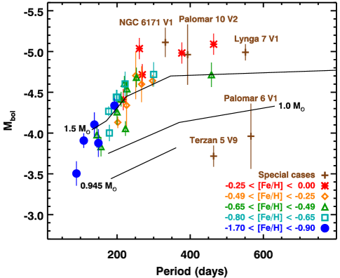
Figure 10 plots the bolometric magnitudes of our sample against their pulsation periods, and it includes (simplified) evolutionary tracks taken from Vassiliadis & Wood (1993, Fig. 20). We will return to this diagram in § 6. Here, the diagram can help us assess cluster membership. Except for two sources in the lower right (Terzan 5 V9 and Palomar 6 V1), the entire sample appears to follow a single sequence from the lower left to the upper right. Terzan 12 V1 is the orange diamond at the lower edge of the sequence with a period of 458 days. It is close enough to the sequence defined by the remaining sources that it validates our choice of distance modulus. The next section examines the three sources that appear below the period-K relation (Figure 9) in turn.
3.3. Special Cases
The bolometric magnitudes of NGC 6171 V1 and Palomar 10 V2 in Table 4 are based on the presumption that they are foreground objects (§ 3.1). If they were actually overtone pulsators and cluster members, their bolometric magnitudes would be 6.85 and 6.52, respectively. According to the evolutionary models of Vassiliadis & Wood (1993), these magnitudes would correspond to initial masses of 5 M☉, much too massive for the age of either cluster.
Terzan 5 V9 is about 1.7 magnitudes too faint at K if it were at the distance of the cluster. Its JK and HK colors, corrected for interstellar extinction, are consistent with 1.2–1.3 magnitudes of circumstellar extinction at K, and its KL color suggests AK1.6. These color-based estimates assume that the circumstellar dust extinction follows the interstellar relationships of Rieke & Lebofsky (1985), and they are roughly consistent with the observed extinction. However, this source sits in the lower right in Figure 10 with P=464 days. If it really is a member of Terzan 5, its bolometric magnitude is inconsistent with its pulsation period. Perhaps it is a background object, or perhaps it is a binary or interacting system. Whatever it is, it is not a normal AGB star, and we consequently do not include it when analyzing the other AGB stars in Terzan 5.
Palomar 6 V1 is too faint by 2.6 magnitudes at K, but its JK, HK, and KL colors correspond to circumstellar extinction at K of 3.5–4.9 magnitudes. These estimates would put the source 1–2 magnitudes of distance modulus in front of Palomar 6. In Figure 10, Palomar 6 V1 is the source below the others in the lower right with P=566 days. If it were in the foreground of Palomar 6, correcting for its distance would push it even further down in Figure 10. Here again, the star cannot be a normal AGB star and a cluster member. As already noted (§2.1), even if it were, the uncertain metallicity of the cluster prevents us from assigning it to one of our metallicity bins.
The spectrum of Lyngå 7 V1 (Figure 8) is unambiguously that of a carbon star, with strong dust emission from SiC at 11.5 m and MgS dust at 26 m, as well as absorption from acetylene gas at 7.5 and 13.7 m. Its carbon-rich status may be consistent with the circumstellar extinction at K apparent in Figure 9, but it would be helpful to independently verify its distance.
We have two means of doing so. Sloan et al. (2008) calibrated a relationship of MK vs. JK color for carbon stars in the SMC, using 2MASS photometry. Correcting the mean magnitudes in Table 2 for interstellar extinction gives JK = 3.71, which leads to a distance modulus of 14.71. Sloan et al. (2008) also found and calibrated a color-magnitude relation for the narrow 6.4- and 9.3-m filters defined to analyze earlier samples of Magellanic carbon stars. Lyngå 7 V1 has a [6.4][9.3] color of 0.55, which implies M9.3=11.59. Since [9.3]=2.67, the distance modulus is 14.26. The average from these two methods is 14.20 0.08, which compares favorably to the nominal distance modulus of Lyngå 7, 14.31555Using an updated calibration of MK vs. JK for the more metal-rich LMC (Lagadec et al., 2010) gives = 14.71 and a mean = 14.49 0.32, which is still close to the nominal distance..
In Figure 10, Lyngå 7 V1 is the upper right datum. Its position is consistent with the evolutionary sequence defined by the larger sample, adding some confidence that it is a cluster member. Nonetheless, its carbon-rich nature prevents any comparison with the oxygen-rich sample, and it remains excluded from most of the analysis in this paper.
3.4. Membership Summary

To summarize, we exclude NGC 6171 V1 and Palomar 10 V2 from the sample because if they were cluster members, they would be too bright for old AGB stars. We exclude Terzan 5 V9 and Palomar 6 V1 from further consideration because if they are cluster members, they are too faint for their pulsation periods compared to the rest of the sample. Finally, while Lyngå 7 V1 is a cluster member, it is a carbon star and must be treated separately from the rest of the sample.
Figure 11 compares the bolometric magnitudes of the 31 LPVs in our sample which are confirmed as members of globular clusters and normal AGB stars to the oxygen-rich Magellanic sample considered by Sloan et al. (2008). The Magellanic sample spans a narrower range of metallicity (0.6 [Fe/H] 0.3). It is readily apparent that the samples represent very different sources. The Magellanic sample consists primarily of supergiants and brighter AGB stars, while the globular sample contains only of fainter and lower-mass AGB stars. This difference arises primarily from the greater distance to the Magellanic Clouds and the resulting bias toward more luminous sources.
4. Spectral Analysis
4.1. Infrared Spectral Classification
The classification of the spectra follows the Hanscom system, defined by Kraemer et al. (2002) for spectra from the Short-Wavelength Spectrometer (SWS) aboard the Infrared Space Observatory (ISO), which is based partially on the classification of spectra of oxygen-rich AGB variables developed by Sloan & Price (1995) for data from the Low-Resolution Spectrograph on the Infrared Astronomical Satellite. Sloan et al. (2008) explained how the method was modified for IRS data from Spitzer. In the Hanscom system, spectra are divided into groups, based on their overall color, and one- or two-letter designations are added to describe the dominant spectral features. All of our spectra fall into Group 1 (for blue spectra dominated by stellar continua and showing no obvious dust), Group 2 (for stars with dust), and Group 3 (for spectra dominated by warm dust emission). Most of our spectra can be classified as either naked stars (“1.N”) or stars showing silicate emission (“2.SE.”).
The classification depends primarily on two quantities. The first quantity is Dust Emission Contrast (DEC), defined as the ratio of the dust excess to the stellar continuum, integrated from 7.67 to 14.03 m. For the stellar continuum, we assume a 3600 K Planck function, fit to the spectrum at 6.8–7.4 m. Sloan & Price (1995, 1998) assumed an Engelke function with 15% SiO absorption at 8 m. Switching to this continuum would systematically shift our DEC measurements upward by 0.04. Table 4 does not include this systematic error in the uncertainties, although it should be kept in mind that the actual stellar continuum could vary from one source to the next. In this sample and with these assumptions, a DEC of 0.10 separates those stars which we visually identify as naked from those with apparent dust excesses.
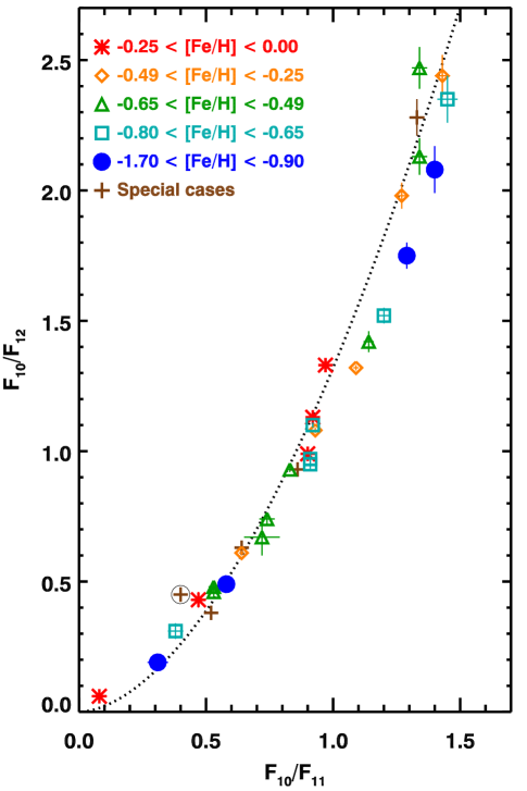
The second quantity, determined for the spectra with an oxygen-rich dust excess, is the ratio of the excess emission at 11 and 12 m (). To measure this flux ratio, we follow the method of Sloan & Price (1995), measuring the excess at 10, 11, and 12 m and plotting the flux ratio as a function of . Figure 12 shows that all oxygen-rich sources fall on or close to the silicate dust sequence, which was defined as a power law: = 1.32 . In the bottom left, the point furthest from the power law is the carbon star Lyngå 7 V1. For the remaining sources, the flux ratio is determined by finding the point on the silicate dust sequence closest to the point defined by the measured ratios and . The corrected ratio defines the silicate emission (SE) index, which runs from 1 for to 8 for . Four sources have positions shifted to the right of the silicate dust sequence in the region where 1.3 1.8; from top to bottom, they are NGC 6712 V7, NGC 6838 V1, NGC 6356 V5, and NGC 6760 V4. Their spectra have typical silicate emission features, and we suspect that the shift arises from a dust component in addition to the usual mixture of amorphous alumina and amorphous silicates.
The corrected flux ratio quantifies the dust composition (Egan & Sloan, 2001). Amorphous alumina dominates the spectra with low flux ratios (or SE indices 1–3), while amorphous silicates dominate the highest flux ratios (SE6–8). For the remainder of the paper, we will use the quanitity to distinguish the spectra by the composition of their dust.
Lyngå 7 V1 is classified in the Hanscom system as “2.CE” (carbon-rich emission). Of the remainder, 10 are naked (“1.N”), and 28 have oxygen-rich dust. Most are classified in the sequence from to “2.SE1” to “2.SE8”, but seven spectra require special attention, as explained next.
Strong silicate self-absorption can push spectra down the silicate dust sequence, as has happened for Palomar 6 V1. This source mimics a 2.SE1 spectrum in Figure 12, but its spectrum (Figure 8) clearly shows self-absorption at 10 m. That, and the fact that the spectrum peaks past 15 m, result in a classification of “3.SB”.
Six of the spectra are distinctly different from the rest and are examined more closely in § 4.5 and 4.6 below. Three clearly show the presence of crystalline silicates in the 10-m feature; they are classified as “SX” instead of “SE”. Three others show an unusual spectral emission feature peaking between 11 and 12 m. To distinguish them from the remainder, we will give them the new (and possibly temporary) classification of “SY”. Both the SX and SY sources are indexed identically to the SE sources, although the interpretation of that index may differ.
The classifications in Table 4 include the suffixes ‘t’, ‘f’, and ‘x’, indicating the presence of a 13-m feature, a 14-m feature, and longer-wavelength features from crystalline silicates, respectively. These emission features and the criteria for their classification are treated in more detail below (§ 4.5 and 4.7).
4.2. Mass-loss Rates
The primary objective of this project is to quantify how the rate of dust production by evolved oxygen-rich stars depends on metallicity. The dust-production rate is identical to the dust mass-loss rate, which is the ratio of the overall mass-loss rate divided by the gas-to-dust ratio. We use two methods to quantify the amount of dust in the circumstellar shell: the DEC described above and the [7][15] color defined by Sloan et al. (2008) and described below. To relate these to the dust mass-loss rate, we use the set of radiative transfer models fitted to 86 evolved stars in the Magellanic Clouds by Groenewegen et al. (2009). Their models determine a dust mass from the opacity needed to fit the IRS spectroscopy and overall spectral energy distribution, assume a constant outflow velocity (10 km s-1) to determine the dust mass-loss rate, and assume a gas-to-dust ratio of 200 to determine the overall mass-loss rate.
The [7][15] color integrates the total flux density (from star and dust) in the wavelength intervals 6.8–7.4 and 14.4–15.0 m. Groenewegen et al. (2009) recently showed that the [7][15] color tracks the mass-loss rate:
| (1) |
They also found that the DEC correlates with mass-loss rate as well:
| (2) |
for mass-loss rates less than 10-5.5 M☉/yr. At higher rates, the shell becomes optically thick enough to drive the 10 m silicate emission feature into self-absorption, and as a result, the DEC breaks down as a useful measure of dust content.
For all sources except the carbon star Lyngå 7 V1 (§ 5.1) and three Cepheids not observed at 15 m, we estimated mass-loss rates using Equations (1) and (2). We began with [7][15] color. For those sources where [7][15] 1.80, indicating a mass-loss rate above 10-5.5 M☉/yr, we used only Equation (1). For those sources below this limit, we also estimated a mass-loss rate from the DEC and averaged the two. We assumed a minimum DEC of 0.0 for the purposes of estimating mass-loss rates.
Table 4 presents the results as overall mass-loss rates, in order to facilitate comparison to other published mass-loss rates. To convert overall mass-loss rate to dust-production rate, one needs to divide by the assumed gas-to-dust ratio of 200, or in log space, to subtract 2.30. For the remainder of the paper, we will focus on the dust-production rate, which avoids assuming a gas-to-dust ratio.
4.3. Dust Production Dependencies

Generally, the mass-loss rate and dust production rate will increase as a star evolves up the AGB, due to the reduced surface gravity and higher luminosity of the central star. This increase will dominate the subtler effect of metallicity. To examine the role of metallicity, one would ideally plot dust production vs. luminosity for samples of different metallicities and compare them. Past comparisons between evolved stars in the Galaxy and the Magellanic Clouds have been hampered by the poorly constrained distances to Galactic sources, and consequently, pulsation period has been used as a proxy for luminosity. Here, we can overcome this difficulty, since the distances to the globular clusters in our sample are known and we can determine bolometric magnitudes directly.
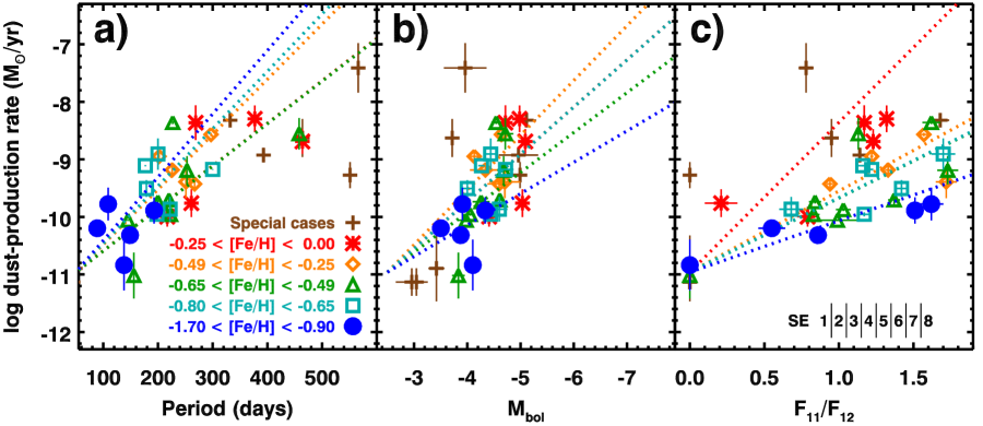
Figure 13 plots the derived mass-loss rates as a function of pulsation period (Panel a), bolometric magnitude (Panel b), and the corrected flux ratio , which quantitifies the dust composition (Panel c). In general, the rate of dust production clearly increases as the stars grow brighter, their pulsation periods increase, or the dust grows more silicate rich. Panel c is analogous to Figure 4 by Sloan & Price (1995), which showed that alumina-rich dust (SE1–3) is seen only in low-contrast shells, while silicate-dominated dust (SE6–8) can exhibit a wide range of dust emission contrasts. The globular sample follows the same trend.
To examine how the metallicity might influence the tendency of the dust production to increase with increasing period, luminosity, or silicate/alumina dust ratio, we have determined a mean slope for each metallicity-defined subsample, including all the spectra depicted in Figures 2 through 7, assuming that they have same y-intercept (which we arbitrarily defined). These slopes appear in Figure 13 as dotted lines. Figure 14 plots the slopes of these fitted lines as a function of metallicity, showing how the metallicity modifies the more obvious relations of dust production with period, luminosity, and dust content. The uncertainties in Figure 14 are the formal uncertainties in the mean (the standard deviation divided by the square root of the sample size; Bevington, 1969).
Panel a in Figures 13 and 14 shows the effect of metallicity when segregating the samples by period, or more to the point, the lack of an effect. While the data may appear to show a negative relation, a horizontal line in Panel a of Figure 14 can touch all of the error bars. This lack of a dependence on metallicity is a little suprising given that Sloan et al. (2008) found a metallicity dependence in dust production when segregating by period and comparing oxygen-rich evolved stars in the Galaxy and the Magellanic Clouds. However, the globular sample spans a wider range of metallicities, and the dependence of pulsation period on metallicity may be obscuring the dependence of dust production on metallicity. One can see in Figure 13 that no star in the most metal-poor bin has a period greater than 200 days, while no star in the most metal-rich bin has a period less than 200 days. The intermediate bins have intermediate periods. Wood (1990) noted that lowering the metallicity of an AGB star raises its effective temperature and thus reduces its radius, which also reduces its pulsation period.
Panel b in Figures 13 and 14 shows that segregating by bolometric magnitude reveals a slight dependence of dust production rates on metallicity, although it is blurred somewhat by scatter in the sample.
The impact of metallicity is clearest when segregating the samples by dust content as measured by (Panel c in the two figures). Whether the dust is alumina-rich or silicate-rich, the dust-production rate increases as the metallicity increases.
Combining the evidence from the three methods of segregating the globular sample, we conclude that metallicity is influencing the rate of dust production by AGB stars. The effect may be stronger than what we observe. Implicit in our calibration of dust-production rate from [7][15] and DEC is the assumption by Groenewegen et al. (2009) that the outflow velocity is 10 km s-1. Recent CO obervations of carbon stars in the Galactic Halo by Lagadec et al. (2010) reveal a possible dependence of the outflow velocity on metallicity. While this result requires confirmation, it is reasonable to consider the possibility that the outflow velocity increases with metallicity in our sample as well. In this case, we would have to revise our dust-production rates upward for the higher metallicities, and the trends in Fig. 13 and 14 would be more apparent.
On the other hand, if the gas-to-dust ratio increases at lower metallicity, this would decrease the dependency for overall mass-loss rate. The likelihood depends on how important the role of dust is in the mass-loss process from the AGB.
4.4. Amorphous alumina
Figure 12 and Figure 13 (Panel c) show that all of the metallicity bins contain spectra classified as SE1–3, which arise from shells dominated by amorphous alumina (Egan & Sloan, 2001). We conclude that AGB stars can produce alumina-rich dust, regardless of their initial metallicity.
Sloan et al. (2008) found little incidence of alumina-rich dust in their Magellanic samples, which they attributed to a possible underabundance of aluminum in more primitive stars, but our detection of alumina-rich dust shells at even lower metallicities repudiates that argument. Sloan & Price (1998) found that Galactic supergiants rarely produced alumina-rich dust shells. Figure 11 shows that the Magellanic sample studied by Sloan et al. (2008) is more luminous, and it follows that it generally contains more massive stars. The lack of low-mass stars in the Magellanic samples may explain the missing alumina-rich dust.
4.5. Warm crystalline dust

| Feature strength/dust strength (%)aaRatio of feature strength to total dust emission from 5 to 35 m; see §4.4. | ||
|---|---|---|
| Target | 13 m | 20 m |
| NGC 362 V2 | 0.70 0.93 | |
| NGC 362 V16 | 0.60 0.21 | |
| NGC 5139 V42 | 0.21 0.08 | |
| NGC 5927 V1 | 1.19 0.09 | 0.70 0.05 |
| NGC 5927 V3 | 0.11 0.01 | 0.07 0.03 |
| NGC 6352 V5 | 0.46 0.10 | 0.60 0.04 |
| NGC 6356 V1 | 0.01 0.01 | |
| NGC 6356 V3 | 0.09 0.24 | |
| NGC 6356 V4 | 0.61 0.31 | 0.23 0.27 |
| NGC 6356 V5 | 0.28 0.12 | |
| Palomar 6 V1 | 0.09 0.03 | |
| Terzan 5 V2 | 0.24 0.13 | |
| Terzan 5 V5 | 0.06 0.07 | 0.13 0.03 |
| Terzan 5 V6 | 0.28 0.02 | 0.49 0.03 |
| Terzan 5 V7 | 0.03 0.01 | 0.16 0.02 |
| Terzan 5 V8 | 0.21 0.11 | 0.80 0.16 |
| Terzan 5 V9 | 0.27 0.03 | 0.35 0.03 |
| NGC 6441 V1 | 1.12 0.20 | 0.93 0.21 |
| NGC 6553 V4 | 0.37 0.06 | 0.24 0.05 |
| IC 1276 V1 | 0.45 0.18 | 0.17 0.06 |
| IC 1276 V3 | 0.23 0.05 | |
| Terzan 12 V1 | 0.08 0.02 | |
| NGC 6637 V4 | 0.07 0.02 | |
| NGC 6712 V2 | 0.04 0.07 | |
| NGC 6760 V3 | 0.32 0.08 | |
| NGC 6760 V4 | 0.10 0.06 | |
| Palomar 10 V2 | 0.22 0.01 | 0.05 0.03 |
| NGC 6838 V1 | 0.32 0.15 | 0.32 0.04 |
| Feature (m) | Continuum intervals (m) | |
|---|---|---|
| 13 | 12.20–12.35 | 13.50–13.65 |
| 20 | 18.40–18.80 | 21.10–21.60 |
Figure 15 shows the three spectra classified as “SX”, based on the splitting of the 10 m-emission feature from amorphous silicate grains into two components at 9.7 and 11.3 m. Sloan et al. (2006) found one source in the LMC which showed similar structure at 10 m, HV 2310, and they showed that an increased fraction of crystalline silicate grains could explain the spectrum. They suggested that grains might form with more crystalline structure in low-density dust-formation zones, as described below. Sloan et al. (2008) added a second source in the LMC: HV 12667.
All three globular SX spectra also show a strong 13-m feature, as well as an additional component at 20 m. These features do not appear in the spectra of HV 2310 or HV 12667 in the LMC. However, at least 24 other spectra in the globular sample show at least one of these features. Table 5 presents the strengths of the features in the spectra where at least one was detected, expressed as a percentage of the total dust emission from 5 to 35 m. We measured these strengths by fitting a line segment over the wavelength ranges given in Table 6 and integrating in between. We repeated the process using a spline to estimate the (dust) continuum, integrating over the same wavelength range. Where both methods produced a continuum that followed the actual data to either side of the feature, we averaged the result. The uncertainties in Table 5 are the larger of the propagated error in the two extractions or the standard deviation between them.
Sloan et al. (2003) found a correlation between the strength of the 13- and 20-m features, quoting a Pearson correlation coefficient of 0.82. We have calculated the same coefficient for all of the sources in the present sample to be 0.62, notably but understandably less given the lower S/N and spectral resolution of the current set of spectra.
Following Sloan et al. (2003), we assign a suffix of “t” to the classification of all sources with a 13 m feature stronger than 0.1% of the total dust emission, provided that the S/N of the detection is 3.0 or more. Where the feature exceeds 0.1% of the total dust, but the S/N is 1.0–3.0, we classify the spectrum as “t:”. Eight spectra have clear 13-m features, and six more have probable 13-m features, which accounts for 14 out of 30 spectra showing oxygen-rich dust emission, or 47%. Nearly all of the variables in the sample are classified as Miras, and Figure 9 reinforces this point. Sloan et al. (1996) estimated that only 20% of Galactic Miras with oxygen-rich dust showed 13-m features; the percentage here is more than twice as high. This difference might be due to the lower masses in the globular sample.
The specific grain which produces the 13-m feature remains an unsettled issue. Whether it is crystalline alumina (corundum; Al2O3), as first proposed by Glaccum (1994), or spinel (MgAl2O4; Posch et al., 1999; Fabian et al., 2001), the groups favoring both candidates agree that an Al–O stretching mode produces the feature (e.g., Lebzelter et al., 2006).
Concentrating on this fact, we can infer that the presence of the 13-m feature indicates the presence of elemental aluminum. The 14 spectra with probable 13-m features are distributed evenly over all metallicities down to [Fe/H]=0.71. Below this metallicity, all but two of the stars are naked, limiting any possible conclusions for that portion of the sample. The presence of aluminum at all metallicities where it can be detected suports the conclusion in § 4.4: The absence of alumina in the Magellanic samples was not a result of different abundances. We see alumina-based dust species in the globular sample at any metallicity where we see oxygen-rich dust.
The difference between corundum vs. spinel as the carrier of the 13-m features boils down to whether or not simple oxide grains like MgO (or perhaps FeO) are actively bonding with the alumina. This difference is important in explaining the 20-m features, since Sloan et al. (2003), who favored corundum, suspected that the latter feature arises from crystalline silicates, while Posch et al. (2002) have proposed an origin in simple oxides ([Mg,Fe]O). In the former case, the presence of the 13- and 20-m features may point to the presence of crystalline analogues to the amorphous alumina and silicates known to form in these dust shells, while in the latter, the two features may indicate a modified chemistry with enhanced oxides. Thus, a resolution of the question would help us understand the pathways followed by the grain chemistry in these dust shells.
The presence of three spectra classified as “SXt” bolsters the case for crystallinity as the origin of the 13- and 20-m features, since we can now see an accompanying enhancement in crystalline olivine at 10 m. These spectra are particularly intriguing, because they help to clarify the origin of the “three-component spectra”, where narrow features at 11 and 13 m are superimposed on the broader 10 m silicate emission feature (Little-Marenin & Little, 1988). Here, we can see the three components more clearly than before.
Sloan et al. (2006), following theoretical arguments by Gail & Sedlmayr (1998), suggested that dust forming at lower densities may have a higher degree of crystallinity. Each photon absorbed by a dust grain will nudge recently accumulated atoms across the surface. If these atoms can be nudged enough times before the accumulation of an overlaying layer locks them into position, then they might fall into lowest energy levels represented by the lattice structure.
A separate mechanism produces crystalline grains at higher mass-loss rates. The higher densities in the dust-formation zone push the condensation temperature higher, and the grains can anneal into a crystalline structure before they cool (see Fabian et al., 2000, and references therein). Thus, crystalline grains could form in cases of either particularly high or particularly low mass-loss rates.
If indeed the appearance of features at 11, 13, 20, and 28 m is due to enhanced crystallinity, one could argue that this is evidence for a disk, which would retain the grains close to the star long enough for them to be radiatively annealed. We believe this is unlikely for most of the sources in our sample because disks would have higher optical depths and more cool dust than observed in these spectra. Generally, self-annealing during formation at low densities is a better explanation than disks.
Palomar 6 V1 may be a different matter. If it is a cluster member, its bolometric magnitude and period are inconsistent with the evolutionary track defined by the AGB stars in this sample (Figure 10 and § 3.3). Its spectrum is probably not produced by outflows from a normal AGB star. The presence of silicate absorption requires high optical depth, which could indicate the presence of an optically thick disk. Grains in such a disk would remain in the star’s vicinity longer than in an outflow, giving them time to be annealed, which could explain the presence of emission features from crystalline silicates at 23, 28, and 33 m.
4.6. Unusual 11–12-m Emission Features

Figure 16 plots the three spectra classified as “SY”, due to a previously unrecognized dust emission feature peaking in the vicinity of 11–12 m. Two of the three sources, NGC 6553 V4 and Terzan 5 V9, also show 13-m features along with a feature at 20 m. Both spectra also show peaks in the emission at 11.5 and 12.2 m. Terzan 12 V1, while having general similarities to the other two spectra, differs in detail, with a single peak in the dust emission at 11.1 m and a relatively normal accompanying 18 m feature.
While the shape of the 11–12-m emission feature is unusual, the flux ratios at 10, 11, and 12 m place the three sources close to the silicate dust sequence in Figure 12 (in the SE1–2 range, with ). Normally, one would expect amorphous alumina to produce spectra with these flux ratios, but we have been unable to duplicate these spectra with optically thin dust shells consisting of only amorphous alumina, or even combinations of amorphous alumina and amorphous silicates. Optically thick models remain untested. It may be worth recalling that one of the three sources, Terzan 5 V9, is something of an enigma (Figure 10), which could possibly be explained by the presence of a disk.
4.7. Narrow Emission Features

Many of the spectra show emission features at 14 m, but the majority of these features are narrower than the 14-m features reported by Sloan et al. (2006, 2008). Only two sources show 14-m features with similar positions and widths to those in these previous papers: NGC 6356 V1 and Palomar 6 V1. They are classified as 2.SE8f and 3.SBfx, respectively. The “x” for Palomar 6 V1 indicates the presence of emission from crystalline silicates at 23, 28, and 33 m. The 14-m dust emission feature tends to be associated with strong amorphous silicate emission, as with NGC 6356 V1, or with crystalline features, as with Palomar 6 V1.
The narrow 14-m features seen in some spectra prevent a thorough search for the slightly broader 14-m feature detected in NGC 6356 V1 and Palomar 6 V1. The narrow 14-m features are centered close to 13.9 m, and some of the most pronounced examples are accompanied by a second emission feature at 16.2 m as well as absorption or emission at 15.0 m. Figure 17 plots some examples.
This combination of spectral features allows us to positively identify the bands as emission from CO2. Justtanont et al. (1998) first identified these bands in spectra from AGB stars obtained with the SWS. The detection of the same bands with the low-resolution modules of the IRS is a bit of a surprise, because its spectral resolution is almost an order of magnitude lower than the SWS. 12CO2 produces narrow emission bands at 13.87, 14.98, and 16.18 m, with the 14.98 m band shifting into absorption in some cases (see Cami et al., 2000). Some spectra also show the emission band seen in SWS data at 13.48 m, as well as an additional band at 16.8 m, which Sloan et al. (2003) argued was also from CO2.
The repeated appearance of features at the right wavelengths in our sample is convincing, even if many of the individual features in individual spectra remain in doubt. Given the noisy nature of the features, we have not attempted a quantitative analysis, though it is worth noting, that most of the sources included in Figure 17 are not 13-m sources. If this result held up with better spectra of globular cluster variables in the future, it would contradict the correlation found by Sloan et al. (2003) for oxygen-rich AGB variables in the Galaxy, where CO2 emission appeared in spectra also showing 13-m features.
4.8. Molecular absorption features


Many of the spectra in the globular sample show clear bands from molecular gas shortward of 10 m. The molecules include SO2 and H2O.
Figure 18 presents six IRS spectra showing absorption from SO2 at 7.3–7.5 m, along with an SWS spectrum of UX Cyg, a Galactic AGB star and one of the first sources in which SO2 was detected (Yamamura et al., 2006). SO2 is the only sulphur-bearing molecule that has been detected in oxygen-rich AGB stars. One would not expect sulpher to be produced in low-mass AGB stars, and it would follow that the strength of the SO2 band should depend on the initial metallicity of the star. Thus, the presence of this band in metal-poor clusters like IC 1276 and NGC 6441, with [Fe/H] = 0.6 or less, is unexpected.
The seven IRS and SWS spectra in Figure 18 also show water vapor absorption at 6.4–6.8 m. Figure 19 presents four more globular spectra with water bands, but no SO2, along with HD 32832, a Galactic M giant also observed with the IRS. This comparison spectrum also shows strong SiO absorption, which is generally absent or weak in the globular sample.
Figures 18 and 19 both contain synthetic absorption spectra based on plane-parallel radiative transfer models (Matsuura et al., 2002a) and line lists from HITRAN (Rothman et al., 2009). These models include only the main isotopes, and the updated line lists provide improved fits to the H2O structure at 6.3 m (Barber et al., 2006). The excitation temperature of the molecules is 1800 K. The absorption in the model in Figure 18 is due entirely to water vapor and SO2. In Figure 19, it is from water vapor and SiO.
Figure 20 presents five more IRS spectra showing an apparent absorption band with a peak opacity 6.35 m. The figure also includes a model showing water vapor in emission, which duplicates reasonably well the structure in the observed spectra. Thus, the “absorption” is actually continuum between emission bands from H2O to either side.
Matsuura et al. (2002a) found that LPVs tend to show water vapor in emission near the maximum of their pulsation cycle, due to detached layers of water vapor in the extended atmosphere. Our five emission sources all have short periods, limiting our certainty of the phase during the IRS observations. The distinguishing characteristic of the emission sources is their periods. All five sources in our sample with periods between 40 and 140 days show water-vapor emission. The variables with longer periods do not.
Tsuji (2001) detected water vapor in K giants, which are warmer than one would expect if the water vapor were in hydrostatic equilibrium. Two of the emission sources in our sample are Cepheids, which are even warmer, and we can conclude that the water vapor around them is probably not in equilibrium.
There has been some unpublished speculation about a possible dust emission feature at 6 m and a possible correlation with other features, such as the 14-m dust emission feature. This “6-m emission feature” extends from 6.0 to 6.5 m with a peak 6.2–6.3 m. It is particularly noticeable in the spectra of NGC 6441 V2 and Terzan 5 V9 in Figure 18. However, the complex spectral structure in the 6-m region created by molecular absorption makes it more likely that this “feature” is really just the continuum between molecular absorption bands.
5. Objects of note
5.1. Lyngå 7 V1
The spectrum of Lyngå 7 V1 clearly identifies it as a carbon star, and our analysis strongly supports its membership in the cluster (3.4). While carbon stars in Galactic globular clusters are rare, they are not unheard of. Wallerstein & Knapp (1998) listed three examples in NGC 5139 ( Cen) and noted that all three were CH stars, which have probably become carbon-rich through mass transfer in a binary system. Côte et al. (1997) discovered a candidate in the cluster M14; it too is a CH star. Lyngå 7 V1 may well be a similar object, which would explain how it could be a member of an old globular cluster and still be a carbon star.
For the sake of completeness, Table 4 includes a mass-loss rate for Lyngå 7 V1 based on its [6.4][9.3] color, the relation of color to dust mass-loss rate defined by Sloan et al. (2008), and an assumed gas-to-dust ratio of 200. Because of its potentially unusual evolutionary path, this mass-loss rate might not be useful for intercomparisons among samples with different metallicities.
5.2. NGC 5139 V42
McDonald et al. (2009) obtained an N-band spectrum of NGC 5139 V42 about four weeks before our IRS observation. Like us, they observed little dust in the spectrum, while earlier mid-infrared photometry (referenced by McDonald et al., 2009) showed a clear excess at 10 m. They concluded that this change in the measurements is likely real. This spectral variation emphasizes the temporal nature of these objects and the importance of obtaining statistically significant samples to average the variations out.
5.3. NGC 362 V2 and V16
Our classification of a star as “naked” means that it does not show an identifiable excess in the 8–14 m region, based on its continuum level in the 5–8 m region. Boyer et al. (2009b) recently detected a photometric excess in two of our “naked” sources, NGC 362 V2 and V16, based on photometry of the continuum at shorter wavelengths. This excess is featureless (at the resolution of the photometry), leading them to identify amorphous carbon as a likely suspect. Because the formation of CO would have left only oxygen to condense into dust in this oxygen-rich environment, the presence of carbon-rich dust would be most unexpected. McDonald et al. (2010), using the spectra presented here, show that iron grains provide the best explanation for the featureless excesses observed in these and other spectra.
5.4. Cepheid variables
Our globular sample includes four Cepheids. All four are type II Cepheids, with periods between 20 and 50 days, taken from the sample by Matsunaga et al. (2006). They could be classified as W Virginis or RV Tauri stars, but the separation between these two groups is ambiguous especially among the globular cluster objects (See Matsunaga et al., 2009).
RV Tau stars are often embedded within circumstellar dust shells (Jura, 1986). Nook & Cardelli (1989) previously reported an infrared excess from one source in our sample, NGC 6626 V17. However, the current IRS spectrum does not show a dust excess around this star, or the other three Cepheids. The difference may arise from temporal variations.
It is interesting that the two Cepheids with longer periods, NGC 6626 V17 and NGC 6779 V6, both show water-vapor emission in their spectra. The Galactic RV Tauri star R Scuti (period 147 days) also shows water-vapor emission (Matsuura et al., 2002b).
6. Evolution on the AGB
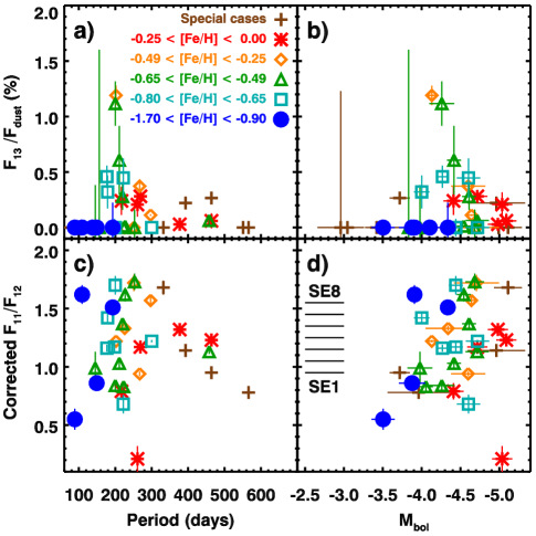
Figure 10 compares the bolometric magnitudes and pulsation periods of the long-period variables in our globular cluster sample to theoretical evolutionary tracks for low-mass AGB stars by Vassiliadis & Wood (1993). The tracks start at the theoretical beginning of the thermally pulsing AGB, and they are roughly consistent with the data from our sample. All of the data appear to follow a mutually consistent evolutionary track, although that track does not follow the theoretical track for either 1.0-M☉ or 1.5-M☉ stars. The two sources which fall to the right of and below the track are Terzan 5 V9 and Palomar 6 V1, and their location away from the rest of the data has already led us to conclude that either they are not actually cluster members, or they are not normal mass-losing AGB stars.
In their study of 47 Tuc, Lebzelter et al. (2006) found that their IRS spectra were consistent with the onset of dust formation at a luminosity of 2000 L☉, which corresponds to , followed by a switch in pulsation mode from an overtone to the fundamental. The dust spectra in their sample showed strong 13-m features at this stage, which then grew comparatively weaker as amorphous silicates begin to dominate. They emphasized the association of a stronger 13-m feature with the fainter and less evolved stars in their sample. Our study cannot address the question of a switch in pulsation mode because all of our long-period variables appear to be pulsating in the fundamental mode, which is consistent with all of our data being brighter than .
Figure 21 tracks the dust properties in our sample with pulsation period and bolometric magnitude. The top panels show that the 13-m feature is most pronounced for pulsators with periods around 200 days and bolometric magnitudes from 3.5 to 4.0. Thus, our globular sample generally conforms to the scenario described by Lebzelter et al. (2006), with the 13-m feature growing weaker and the contribution from amorphous silicates increasing as the star evolves along the AGB. We do not see any evidence for sudden shifts in spectral properties, but then our sample shows no shift from overtone to fundamental mode, as seen in 47 Tuc.
The bottom panels of Figure 21 show little dependence of the corrected flux ratio with either period or bolometric luminosity. We have noted previously that Galactic supergiants and the luminous AGB stars and supergiants observed in the Magellanic Clouds show little sign of amorphous alumina in their spectra. The globular sample, though, is restricted to lower luminosities, and within that range, amorphous alumina and amorphous silicates can dominate the shells with little apparent dependence on either period or luminosity.
7. Summary
We have presented the infrared spectra of a sample of 39 variable stars in 23 globular clusters. The sample includes four Cepheid variables, none of which show dust in their spectra, and 35 long-period variables, of which we can confirm 31 as members of their clusters. These stars are either naked, show emission from oxygen-rich dust, or in one case, show emission from carbon-rich dust. The variety of dust species is impressive, and we see amorphous silicates, amorphous alumina, emission from crystalline grains at several wavelengths, and three spectra which we have not yet been able to characterize. The spectra are also rich in molecular features, including absorption from H2O and SO2, and emission from H2O and CO2.
The main objective of this paper is to probe how the quantity and composition of the dust depend on metallicity. Our sample shows dust emission over the range 0.97 [Fe/H] 0.08. Across this range, stars with lower metallicities generally have less dust in their circumstellar shells. This trend is most readily apparent when plotting (dust) mass-loss rate as a function of the dust composition (as quantified by the flux ratio ), but it is also noticeable when plotting mass-loss rate vs. bolometric magnitude. The lack of a metallicity trend vs. pulsation period may arise from dependencies of the period on metallicity.
We find contributions from alumina-rich dust at every metallicity at which we see silicates. This result indicates that the lack of alumina in the Magellanic samples published thus far is most likely a selection effect, since those samples do not include objects as intrinsically faint as those published here, and the brighter objects tend to show mostly silicates.
Three spectra have a 10 m-emission feature split into components at 9.7 and 11.3 m, along with a strong 13-m feature. The splitting at 10 m is reminicent of two spectra in the LMC which Sloan et al. (2008) fitted with crystalline analogues of the amorphous silicates which produce the broad 10-m feature. These spectra support the case that the 13-m feature arises from the crystalline analogue of the amorphous alumina seen in several other spectra.
This initial paper has only scratched the surface of a rich set of spectroscopic data. A careful mineralogical analysis of the dust features should help address some of the questions left unanswered here. In addition, the spectra are rich in molecular features, both in the 5–8-m region and in the 13.5–17 m region. Detailed modelling will give us insight about the behavior fo these molecules in metal-poor environments.
While Spitzer has exhausted its cryogens and the IRS no longer operates, there is still a strong need for further infrared spectra of evolved stars in globular clusters. The sample here is only large enough to point to trends of fundamental importance. The need for more data and larger samples is clear.
References
- Alves (2004) Alves, D. R. 2004, New Astr. Rev., 48, 659
- Barber et al. (2006) Barber, R. J., Tennyson, J., Harris, G. J., Tolchenov, R. N. 2006, MNRAS, 368, 1087
- Barbuy et al. (1998a) Barbuy, B., Bica, E., & Ortolani, S. 1998a, A&A, 333, 117
- Barbuy et al. (1998b) Barbuy, B., Ortolani, S., & Bica, E. 1998b, A&AS, 132, 333
- Bevington (1969) Bevington, P. R. 1969, Data Reduction and Error Analysis for the Physical Sciences (New York: McGraw-Hill)
- Boyer et al. (2009a) Boyer, M. L., Skillman, E. D., van Loon, J. Th., Gehrz, R.D., & Woodward, C. E. 2009a, ApJ, 697, 1993
- Boyer et al. (2009b) Boyer, M. L., et al. 2009b, ApJ, 705, 746
- Cami et al. (2000) Cami, J., Yamamura, I., de Jong, T., Tielens, A. G. G. M., Justtanont, K., & Waters, L. B. F. M. 2000, A&A, 360, 562
- Caputo et al. (2002) Caputo, F., Degl’Innocenti, S., & Marconi, M. 2002, in ASP Conf. Ser. 265, omega Centauri, A Unique Window into Astrophysics, ed. F. van Leeuwen, J. D. Hughes, & G. Piotto (San Francisco: ASP), 185
- Carretta et al. (2007) Carretta, E., Bragaglia, A., Gratton, R. G., Momany, Y., Recio-Blanco, A., Cassisi, S., François, P., James, G., Lucatello, S., & Moehler, S. 2007, A&A, 464, 967
- Carretta et al. (2009) Carretta, E., Bragaglia, A., Gratton, R., D’Orazi, V., & Lucatello, S. 2009, A&A, 508, 695
- Carretta & Gratton (1997) Carretta, E. & Gratton, R. G. 1997, A&AS, 121, 95
- Carretta et al. (2000) Carretta, E., Gratton, R. G., Clementini, G., & Fusi Pecci, F. 2000, ApJ, 533, 215
- Catelan (2006) Catelan, M. 2006, in ASP Conf. Ser., Resolved Stellar Populations, ed. D. Valls-Gabaud & M. Chavez (San Francisco: ASP), in press
- Clement et al. (2001) Clement, C., Muzzin, A., Dufton, Q., Ponnampalam, T., Wang, J., Burford, J., Richardson, A., Rosebery, T., Rowe, J., & Hogg, H. S. 2001, AJ, 122, 2587
- Côte et al. (1997) Côte, P., Hanes, D. A., McLaughlin, D. E., Bridges, T. J., Hesser, J. E., & Harris, G. L. H. 1997, ApJ, 476, L15
- Dalessandro et al. (2008) Dalessandro, E., Lanzoni, B., Ferraro, F. R., Rood, R. T., Milone, A., Piotto, G., & Valenti, E. 2008, ApJ, 677, 1069
- Del Principe et al. (2006) Del Principe, M., et al. 2006, ApJ, 652, 362
- Dotter et al. (2010) Dotter, A., Sarajedini, A., Anderson, J., Aparicio, A., Bedin, L. R., Chaboyer, B., Majewski, S., Mar n-Franch, A., Milone, A., Paust, N., Piotto, G., Reid, I. N., Rosenberg, A., & Siegel, M. 2010, ApJ, 708, 698
- Egan & Sloan (2001) Egan, M. P. & Sloan, G. C. 2001, ApJ, 558, 165
- Fabian et al. (2000) Fabian, D., Jäger, C., Henning, Th., Dorschner, J., Mutschke, H. 2000, A&A, 364, 282
- Fabian et al. (2001) Fabian, D., Posch, Th., Mutschke, H., Kerschbaum, F., & Dorschner, J. 2001, A&A, 373, 1125
- Ferraro et al. (1999) Ferraro, F. R., Messineo, M., Fusi Pecci, F., De Palo, M. A., Straniero, O., Chieffi, A., & Limongi, M. 1999, AJ, 118, 1738
- Ferraro et al. (2009) Ferror, F. R., Dalessandro, E., Mucciarelli, A., Beccari, G., Rich, R. M., Origlia, L., Lanzoni, B., Rood, R. T., Valenti, E., Bellazzini, M., Ransom, S. M., & Cocozza, G. 2009, Nature, 462, 483
- Gail & Sedlmayr (1998) Gail, H.-P., & Sedlmayr, E. 1998, in The Molecular Astrophysics of Stars and Galaxies, ed. T. W. Hartquist & D. A. Williams (Oxford: Clarendon Press), 285
- Glaccum (1994) Glaccum, W. 1994, in Proc. of the Airborne Astronomy Symp. on the Galactic Ecosystem: From Gas to Stars to Dust, ed. M. R. Haas, J. A. Davidson, & E. F. Erickson (San Francisco: ASP), 395
- Gratton et al. (1997) Gratton, R. G., Fusi Pecci, F., Carretta, E., Clementini, G., Corsi, C. E., & Lattanzi, M. 1997, ApJ, 491, 749
- Groenewegen et al. (2007) Groenewegen, M. A. T., et al. 2007, MNRAS, 376, 313
- Groenewegen et al. (2009) Groenewegen, M. A. T., Sloan, G. C., Soszyński, I., & Petersen, E. 2009, A&A, 506, 1277
- Harris (1996) Harris, W. E. 1996, AJ, 112, 1487
- Harris (2003) Harris, W. E. 2003, revision of Harris (1996) published online: http://www.physics.mcmaster.ca/Globular.html
- Heitsch & Richtler (1999) Heitsch, F. & Richtler, T. 1999, A&A, 347, 455
- Higdon et al. (2004) Higdon, S. J. U., Devost, D., Higdon, J. L., Brandl, B. R., Houck, J. R., Hall, P., Barry, D., Charmandaris, V., Smith, J. D. T., Sloan, G. C., & Green, J. 2004, PASP, 116, 975
- Houck et al. (2004) Houck, J. R., et al. 2004, ApJS, 154, 18
- Iben & Renzini (1983) Iben, I., Jr. & Renzini, A. 1983, ARA&A, 27, 271
- Ivanov et al. (2000) Ivanov, V. D., Borissova, J., Alonso-Herrero, A., & Russeva, T. 2000, AJ, 119, 2274
- Jura (1986) Jura, M. 1986, ApJ, 309, 732
- Justtanont et al. (1998) Justtanont, K., Feuchtgruber, H., de Jong, T., Cami, J., Waters, L. B. F. M., Yamamura, I., & Onaka, T. 1998, A&A, 330, L17
- Kaisler et al. (1997) Kaisler, D., Harris, W.E., & McLaughlin, D. E. 1997, PASP, 109, 920
- Kaluzny et al. (2002) Kaluzny, J., Thompson, I., Krzeminski, W., Olech, A., Pych, W., & Mochejska, B. 2002, in ASP Conf. Ser. 265, omega Centauri, A Unique Window into Astrophysics, ed. F. van Leeuwen, J. D. Hughes, & G. Piotto (San Francisco: ASP), 145
- Karakas & Lattanzio (2007) Karakas, A. & Lattanzio, J. C. 2007, Publ. Astron. Soc. Australia, 24, 103
- Keller & Wood (2006) Keller, S. C. & Wood, P. R. 2006, ApJ, 642, 834
- Kraemer et al. (2002) Kraemer, K. E., Sloan, G. C., Price, S. D., & Walker, H. J. 2002, ApJS, 140, 389
- Lagadec et al. (2010) Lagadec, E., Zijlstra, A. A., Mauron, N., Fuller, G., Josselin, E., Sloan, G. C., Riggs, A. J. E. 2010 MNRAS, 303, 1331
- Lebouteiller et al. (2010) Lebouteiller, V., Bernard-Salas, J., Sloan, G. C., & Barry, D. J. 2010, PASP, 122, 231
- Lebzelter et al. (2006) Lebzelter, Th., Posch, Th., Hinkle, K., Wood, P. R., & Bouwman, J. 2006, ApJ, 653, L145
- Lee & Carney (2002) Lee, J.-W. & Carney, B. W. 2002, AJ, 123, 3305
- Little-Marenin & Little (1988) Little-Marenin, I. R., & Little, S. J. 1988, ApJ, 303, 305
- Matsunaga (2007a) Matsunaga, N. 2007, Ph.D. Thesis, Univ. of Tokyo
- Matsunaga (2007b) Matsunaga, N. 2007b, in ASP Conf. Ser. 378, Why Galaxies Care about AGB Stars: Their Importance as Actors and Probes, ed. F. Kerschbaum, C. Charbonnel, & R. F. Wing. (San Francisco: ASP), 86
- Matsunaga et al. (2009) Matsunaga, N., Feast, M. W., & Menzies, J. W. 2009, MNRAS, 397, 933
- Matsunaga et al. (2006) Matsunaga, N., Fukushi, H., Nakada, Y., Tanabé, T., Feast, M. W., Menzies, J. W., Ita, Y., Nishiyama, S., Baba, D., Naoi, T., Nakaya, H., Kawadu, T., Ishihara, A., & Kato, D. 2006, MNRAS, 370, 1979
- Matsuura et al. (2002a) Matsuura, M., Yamamura, I., Cami, J., Onaka, T., & Murakami, H. 2002a, A&A, 383, 972
- Matsuura et al. (2002b) Matsuura, M., Yamamura, I., Zijlsta, A. A., & Bedding, T. R. 2002b, A&A, 387, 1022
- McDonald et al. (2010) McDonald, I., Sloan, G. C., Zijlstra, A. A., Matsunaga, N., Matsuura, M., Kraemer, K. E., Bernard-Salas, J., & Markwick, A. J. 2010, ApJLetters, in press
- McDonald et al. (2009) McDonald, I., van Loon, J. Th., Decin, L., Boyer, M. L., Dupree, A. K., Evans, A., Gehrz, R. D., & Woodward, C. E. 2009, MNRAS, 394, 831
- McGregor (1994) McGregor, P. J. 1994, PASP, 106, 508
- McGregor et al. (1994) McGregor, P. J., Hart, J., Hoadley, D., & Bloxham, G. 1994, in Infrared Astronomy with Arrays, ed. I. McLean (Dordrecht: Kluwer), 299
- McNamara (2000) McNamara, D. H. 2000, PASP, 112, 1096
- Minniti (1995) Minniti, D. 1995, A&A, 303, 468
- Morgan & Dickerson (2000) Morgan, S. M. & Dickerson, C. 2000, Acta Astron., 50, 249
- Nagayama et al. (2003) Nagayama, T., Nagashima, C., Nakajima, Y., Nagata, T., Sato, S., Nakaya, H., Yamamuro, T., Sugitani, K., & Tamura, M. 2003, Proc. SPIE, 4841, 459
- Nook & Cardelli (1989) Nook, M. A., & Cardelli, J. A. 1989, ApJ, 346, L29
- Origlia & Rich (2004) Origlia, L. & Rich, R. M. 2004, AJ, 127, 3422
- Ortolani et al. (2007) Ortolani S., Barbuy, B., Bica, E., Zoccali, M., & Renzini, A. 2007, A&A, 470, 1043
- Ortolani et al. (1998) Ortolani, S., Bica, E., & Barbuy, B. 1998, A&AS, 127, 471
- Posch et al. (2002) Posch, Th., Kerschbaum, F., Mutschke, H., Dorschner, J., & Jäger, C. 2002, A&A, 393, 7P
- Posch et al. (1999) Posch, T., Kerschbaum, F., Mutschke, H., Fabian, D., Dorschner, J., & Hron, J. 1999, A&A, 352, 609
- Recio-Blanco et al. (2005) Recio-Blanco, A., Piotto, G., de Angeli, F., Cassisi, S., Riello, M., Salaris, M., Pietriferni, A., Zoccali, M., & Aparicio, A. 2005, A&A, 432, 851
- Rieke & Lebofsky (1985) Rieke, G. H. & Lebofsky, M. J. 1985, ApJ, 288, 618
- Rothman et al. (2009) Rothman L. S., et al. 2009, Journal of Quantitative Spectroscopy & Radiative Transfer, 110, 533
- Salaris & Weiss (1998) Salaris, M. & Weiss, A. 1998, A&A, 335, 943
- Salpeter (1952) Salpeter, E. E. 1952, ApJ, 115, 326
- Sarajedini (2004) Sarajedini, A. 2004, AJ, 128, 1228
- Skrutskie et al. (2006) Skrutskie, M. F., et al. 2006, AJ, 131, 1163
- Sloan et al. (2006) Sloan, G. C., Devost, D., Bernard-Salas, J., Wood, P. R., & Houck, J. R. 2006, ApJ, 638, 472
- Sloan et al. (2003) Sloan, G. C., Kraemer, K. E., Price, S. D., & Shipman, R. F. 2003, ApJS, 147, 379
- Sloan et al. (2008) Sloan, G. C., Kraemer, K. E., Wood, P. R., Zijlstra, A. A., Bernard-Salas, J., Devost, D., Houck, J. R. 2008, ApJ, 686, 1056
- Sloan et al. (1996) Sloan, G. C., LeVan, P. D., & Little-Marenin, I. R. 1996, ApJ, 463, 310
- Sloan et al. (2009) Sloan, G. C., Matsuura, M., Zijlstra, A. A., Lagadec, E., Groenewegen, M. A. T., Wood, P. R., Szyszka, C., Bernard-Salas, J., & van Loon, J. Th. 2009, Science, 323, 353
- Sloan & Price (1995) Sloan, G. C. & Price, S.D. 1995, ApJ, 451, 758
- Sloan & Price (1998) Sloan, G. C. & Price, S.D. 1998, ApJS, 119, 141
- Sloan et al. (2010) Sloan, G. C., et al. 2010, in prep.
- Smith (2003) Smith, B. J. 2003, AJ, 126, 935
- Stephens & Frogel (2004) Stephens, A. W. & Frogel, J. A. 2004, AJ, 127, 925
- Thompson et al. (2001) Thompson, I. B., Kaluzny, J., Pych, W., Burley, G., Krzeminski, W., Paczyński, B., Persson, S. E., & Preston, G. W. 2001, AJ, 121, 3089
- Tsuji (2000) Tsuji, T. 2000, ApJ, 540, L99
- Tsuji (2001) Tsuji, T. 2001, A&A, 376, L1
- Valenti et al. (2004) Valenti, E., Ferraro, F. R., & Origlia, L. 2004, MNRAS, 351, 1204
- Valenti et al. (2007) Valenti, E., Ferraro, F. R., & Origlia, L. 2007, AJ, 133, 1278
- Valenti et al. (2005) Valenti, E., Origlia, L., & Ferraro, F. R. 2005, MNRAS, 361, 272
- van de Ven et al. (2006) van de Ven, G., van den Bosch, R. C. E., Verolme, E. K., & de Zeeuw, P. T. 2006, A&A, 445, 513
- Vassiliadis & Wood (1993) Vassiliadis, E. & Wood, P. R. 1993, ApJ, 413, 641
- Wallerstein & Knapp (1998) Wallerstein, G. & Knapp, G. R. 1998, ARA&A, 36, 369
- Werner et al. (2004) Werner, M. W., et al. 2004, ApJS, 154, 1
- Whitelock et al. (2008) Whitelock, P. A., Feast, M. W., & van Leeuwen, F. 2008, MNRAS, 386, 313
- Wood (1990) Wood, P. R. 1990, in From Miras to planetary nebulae: Which path for stellar evolution?, ed. M. O. Mennessier & A. Omont (Gif-sur-Yvette: Editions Frontieres), 67
- Yamamura et al. (2006) Yamamura, I., de Jong, T., Onaka, T., Cami, J., & Waters, L. B. F. M. 2006, A&A, 341, L9
- Zinn (1985) Zinn, R. 1985, ApJ, 293, 424