Parsec-scale Faraday Rotation Measures
from General Relativistic MHD Simulations of Active Galactic Nuclei Jets

Abstract

For the first time it has become possible to compare global 3D general relativistic magnetohydrodynamic (GRMHD) jet formation simulations directly to very-long baseline interferometric multi-frequency polarization observations of the ${\rm pc}$-scale structure of active galactic nucleus (AGN) jets. Unlike the jet emission, which requires post hoc modeling of the non-thermal electrons, the Faraday rotation measures (${\rm RM}$s) depend primarily upon simulated quantities and thus provide a robust way in which to confront simulations with observations. We compute ${\rm RM}$ distributions of 3D global GRMHD jet formation simulations, with which we explore the dependence upon model and observational parameters, emphasizing the signatures of structures generic to the theory of MHD jets. With typical parameters, we find that it is possible to reproduce the observed magnitudes and many of the structures found in AGN jet ${\rm RM}$s, including the presence of transverse ${\rm RM}$ gradients. In our simulations the ${\rm RM}$s are generated within a smooth extension of the jet itself, containing ordered toroidally dominated magnetic fields. This results in a particular bilateral morphology that is unlikely to arise due to Faraday rotation in distant foreground clouds. However, critical to efforts to probe the Faraday screen will be resolving the transverse jet structure. Therefore, the ${\rm RM}$s of radio cores may not be reliable indicators of the properties of the rotating medium. Finally, we are able to constrain the particle content of the jet, finding that at ${\rm pc}$-scales AGN jets are electromagnetically dominated, with roughly 2% of the comoving energy in nonthermal leptons and much less in baryons.

1 Introduction

Spatially resolved radio images of the polarized emission of active galactic nucleus (AGN) jets on ${\rm pc}$-scales, obtained via very-long baseline interferometry (VLBI), have provided a wealth of information regarding the large-scale structure of jet magnetic fields within the emission region. For many objects these observations suggest the presence of large-scale, radially-correlated, toroidally dominant magnetic fields within the emission region (Udomprasert et al., 1997; Lister et al., 1998; Gabuzda et al., 2000; Pushkarev et al., 2005; Jorstad et al., 2005), in broad qualitative agreement with simple analytical models of relativistic magnetized outflows (e.g., Laing & Bridle, 2002b, a; Lyutikov et al., 2005; Zakamska et al., 2008).

Performing these observations often requires removing the rotation of the polarization angle, $\Psi$, associated with Faraday rotation, a consequence of propagation through intervening, non-radiating plasma. If the entirety of the Faraday rotation occurs in the foreground, ignoring finite beam effects, the observed polarization angle at a wavelength, $\lambda$, is related to the intrinsic polarization angle via,

$$\Psi_{\rm obs}=\Psi_{\rm int}+{\rm RM}\lambda^{2}\,,$$ (1)

where the Faraday rotation measure, ${\rm RM}$, is independent of wavelength and has a value that depends upon the plasma parameters along a given line of sight. In practice, eliminating the Faraday rotation requires imaging the source at a number of wavelengths, accurately registering each image to an absolute reference frame, verifying at each independent position within the image that the polarization angles follow the expected $\lambda^{2}$ law and fitting to obtain a map of the ${\rm RM}$s across the image. Despite the difficulty in performing these measurements, ${\rm pc}$-scale ${\rm RM}$ maps for a number of blazars and BL Lac objects can now be found in the literature (Reynolds et al., 2001; Zhang & Nan, 2001; Zavala & Taylor, 2001; Asada et al., 2002; Zavala & Taylor, 2002, 2003; Gabuzda & Chernetskii, 2003; Cotton et al., 2003; Zavala & Taylor, 2004; Asada et al., 2004; Gabuzda et al., 2004; Zavala & Taylor, 2005; Asada et al., 2008a, b, c; Gómez et al., 2008; O’Sullivan & Gabuzda, 2009b; Kharb et al., 2009; Croke et al., 2010).

Typical values of the ${\rm RM}$s of AGN jets range from roughly $1\,{\rm rad}\,{\rm m}^{-2}$ to $10^{4}\,{\rm rad}\,{\rm m}^{-2}$, with extreme core ${\rm RM}$s of $10^{5}\,{\rm rad}\,{\rm m}^{-2}$ being observed in a handful of sources (though these are generally at the centers of cooling core clusters). While the measuring of ${\rm RM}$s allows the elimination of a foreground effect upon the structure of the polarization of AGN jets, it also presents an opportunity to study the intervening, non-radiating plasma. The source of the ${\rm RM}$s is not a priori clear, with potential contributions arising from propagation through the Galactic interstellar medium, intracluster medium, the galactic halo of the AGN, the AGN broad-line region and through the circum-jet environment. It is this last possibility, propagation through the plasma immediately surrounding the jet, that is the subject of this paper.

Free-free absorption from ${\rm pc}$-scale foreground clouds has been detected in a handful of sources, implying that foreground clouds exist and may be responsible for a significant fraction of the observed ${\rm RM}$s in some systems (e.g., Cen A and NGC, Jones et al., 1996; Walker et al., 2000), though there is no reason to expect these to result in ordered ${\rm RM}$ maps exhibiting gradients that are correlated with other aspects of the jet structure. In contrast, there are a number of reasons to think that the circum-jet environment is responsible for substantial fraction of the AGN jet ${\rm RM}$s. Firstly, there is considerable structure on the scale of the resolved jet, which is unlikely to arise from Galactic or intergalactic propagation. Second, in many sources there is a clear gradient in the ${\rm RM}$ values along the jet axis, steeply decreasing with increasing distance from the radio core. Finally, in a handful of objects (e.g., 3C 273, Zavala & Taylor, 2001; Asada et al., 2002; Gabuzda et al., 2004; Zavala & Taylor, 2005; Asada et al., 2008a, b) there is now strong evidence for transverse ${\rm RM}$ gradients, which have thus far been interpreted in the context of a circum-jet Faraday screen containing large-scale toroidal magnetic fields (Blandford, 1993; Gabuzda et al., 2000; Broderick & Loeb, 2009).

Magnetic tower models are often invoked to provide a reasonable basis for the presence of helical fields in relativistic jets. However, models identified as magnetic tower types in the literature are non-relativistic models (Koenigl & Choudhuri, 1985; Lynden-Bell, 1996; Nakamura et al., 2001; Lovelace et al., 2002) and thus are not directly applicable to astrophysical jets (Lyutikov et al., 2005). Nevertheless, non-relativistic simulations of magnetic tower models suggest that the ${\rm RM}$s are strongly influenced by the toroidal magnetic field, and correlated with the large-scale jet structure (Nakamura et al., 2001; Kigure et al., 2004; Uchida et al., 2004; Lapenta & Kronberg, 2005a; Nakamura et al., 2008). Comparisons between idealized, qualitative magnetohydrodynamic (MHD) models (Laing et al., 2006b, a) and observations of ${\rm k}{\rm pc}$-scale polarized emission from FRI jets suggest that in addition to an ordered toroidal magnetic field, at these distances such jets must also contain a smaller, though still significant, disordered poloidal field. However, at such large distances FRI jets are strongly affected by their interaction with the external medium, and thus these results may have little to do with the ${\rm pc}$-scale, intrinsic structure of AGN jets in general.

Self-consistent quantitative models of idealized relativistic MHD jets have been obtained more recently using a combination of analytical modelling (Vlahakis & Königl, 2004) and time-dependent simulations (Komissarov et al., 2007; Tchekhovskoy et al., 2009a, b). However, such idealized simulations cannot consider the self-consistent formation of the jet by the black hole interacting with an accretion disk or the effects of magnetic field geometry and turbulence within the disk. Idealized studies cannot, e.g., self-consistently determine the effects of black hole spin on the jet power for a given mass accretion rate. In contrast, modern general relativistic magnetohydrodynamical (GRMHD) simulations of accreting black holes allow a study of the self-consistent generation of relativistic jets from rotating, accreting black holes (McKinney, 2006; Hawley & Krolik, 2006; Beckwith et al., 2008; McKinney & Blandford, 2009). GRMHD simulations allow one to study the conditions under which relativistic jets are produced, including the role of the magnetic field geometry near the black hole and how MHD turbulence affects the formation of the jet from the black hole or the wind from the turbulent disk (McKinney & Gammie, 2004; Beckwith et al., 2008; McKinney & Blandford, 2009). Such simulations find that an ordered (but not necessarily large-scale) dipole-like magnetic field within the accretion disk leads to a quasi-steady relativistic outflow powered by the Blandford-Znajek mechanism (Blandford & Znajek, 1977; McKinney & Gammie, 2004). While such jets are dominated by a toroidal magnetic field, they remain stable against the disruptive helical kink (screw) mode due to relativistic rotation of magnetic field lines, sideways (lateral) expansion, finite mass-loading, and non-linear saturation (McKinney & Blandford, 2009).

Synchrotron emission maps have been produced for highly-idealized relativistic magnetized jet models (Lyutikov et al., 2005; Zakamska et al., 2008; Gracia et al., 2009), but they generally have major simplifying assumptions, such as perfect cylindrical geometry, self-similarity, only solving for the asymptotic structure (which is unconstrained relative to the self-consistent global solution that would include the region near the disk), treating the accretion disk as a boundary condition, or ignoring gravity altogether. As far as the authors are aware, none of the advanced, but still somewhat idealized, relativistic MHD jet simulations (Komissarov et al., 2007; Tchekhovskoy et al., 2009a, b) have been used to study the emission from AGN jets. Moreover, in light of the lack of an ab initio understanding of particle acceleration within AGN jets, all efforts to model the jet emission require ad hoc prescriptions for inserting the emitting particles.

Unlike emission maps, the ${\rm RM}$ maps depend only upon the velocity, magnetic field, thermal ion density and electron temperature. As a consequence MHD simulations are well-suited to computing ${\rm RM}$s without additional assumptions. Already, global axisymmetric MHD simulations have been used to constrain the mass accretion rate and magnetic field geometry of the supermassive black hole in the Galactic center (Sharma et al., 2007). Computing the ${\rm RM}$s of AGN jets requires the self-consistent simulating of both the emitting fast jet core and the surrounding Faraday screen. However, this is naturally accomplished by GRMHD simulations of jet formation, which generally produce a variety of outflow components, including an ultra-relativistic jet and a surrounding trans-relativistic wind (McKinney, 2006).

Here we present the first analyses of ${\rm pc}$-scale ${\rm RM}$s associated with self-consistent 3D GRMHD simulations of relativistic jets. For this purpose, we employ the fully 3D GRMHD simulation reported by McKinney & Blandford (2009), and perform polarized radiative transfer through the 3D volume, generating frequency-dependent polarized flux maps and ${\rm RM}$s. We investigate how these depend upon model, observational and physical parameters, paying specific attention to how Faraday rotation within the circum-jet plasma may be distinguished from that due to distant Faraday screens. Section 2 summarizes the computational modeling, including the GRMHD simulation, radiative transfer and beam convolution computations. Section 3 presents ${\rm RM}$ maps for a variety of model parameters and describes the implications for the location and structure of Faraday screen, as well as our theoretical understanding of jet formation. Finally, our conclusions are summarized in Section 4.

2 Computational Methods

A number of factors affect the computation of the ${\rm RM}$ maps of simulated jets. Foremost among these is the location, structure and dynamical state of the Faraday screen itself, which we will find to be naturally generated by the circum-jet material immediately surrounding the jet. However, in addition we must also carefully account for the relativistic motion within the Faraday screen, the suppression of Faraday rotation at high electron temperatures, finite radio-beam effects and even the location and mechanism responsible for producing the observed jet emission. In this section we describe how we do each.

2.1 GRMHD Simulations

To model the jet system, we use the fully 3D (no assumed symmetries) general relativistic (GRMHD) simulations reported in McKinney & Blandford (2009). We will only summarize the aspects that are relevant to our present application here. The simulations were generated using the conservative, shock-capturing GRMHD scheme HARM (Gammie et al., 2003) to simulate the evolution of an accretion flow around a rotating black hole, and the subsequent self-consistent generation of bipolar relativistic outflows. Given an initially dipole magnetic field, embedded within the accretion disk near the black hole with spin $a/M\approx 0.92$, they have found that generally a quasi-stable relativistic jet develops and propagates to large radii. While in general many different black hole spins could be considered, models with $a/M\gtrsim 0.4$ are qualitatively similar to those with $a/M\approx 0.92$ (McKinney, 2005). The simulations run for a duration of about $5\times 10^{3}GM/c^{3}$, by which the jet has passed beyond the simulation box, which has a radius of $10^{3}GM/c^{2}$. The baryon density at the base of the jet, very close to the rotating black hole, is determined by limiting the comoving electromagnetic energy density per rest-mass energy density to no larger than $100$, which strictly limits the Lorentz factor to less than order $100$. The accretion disk has a finite extent of about $r\sim 40M$, which limits the radial range (order $r\sim 100M$) over which the jet is collimated by the disk, corona, and disk-driven wind. This finite collimation extent leads to a saturation of the Lorentz factor at roughly 5–10. The effect of a more or less extended disk, and so larger or small terminal Lorentz factors, respectively, can be considered in future work. The jet near the black hole is perturbed by disk-driven turbulence that induces substructure dominated by the $|m|=1$ (where $m$ is the azimuthal quantum number) mode at any given radius, and there is also substantial power in other spherical harmonics. Varying amplitudes of these modes are advected with the jet velocity and become part of the jet substructure at large radii. A single snapshot at $t=2750GM/c^{3}$ was used from the simulation data, which is a time corresponding to after the jet has fully developed inside the computational box but the flow has not significantly reflected off the box.

The simulations are completely described by the gas rest-mass density, $\rho$, the gas internal energy, $u_{g}$ (gas pressure $p_{g}=\left(\Gamma_{g}-1\right)u_{g}$), the lab-frame velocities $\rm\beta$, the comoving magnetic fields, $\rm b$, and the spacetime geometry (defined by the metric components, $g_{\mu\nu}$). While these simulations assume an ideal gas equation of state, with a fixed adiabatic index of $\Gamma_{g}=4/3$, variations in the adiabatic index do not significantly change the dynamics of highly magnetized jets (McKinney & Gammie, 2004). From these quantities one can compute the baryon number density, $n\equiv\rho/m_{b}$ (where $m_{b}$ is the baryon mass) and the ideal gas temperature, $T=p_{g}/nk$ (where $k$ is Boltzmann’s constant). Since we are interested in rapidly accreting, and therefore well-coupled, systems, we assume that the electron and ion temperatures are the same. Finally, note that the lab-frame and comoving magnetic fields are related by

$$\mbox{\boldmath$\rm B$}=\Gamma\left(\mbox{\boldmath$\rm 1$}-\mbox{\boldmath$\rm\beta$}\mbox{\boldmath$\rm\beta$}\right)\cdot\mbox{\boldmath$\rm b$}\quad\Leftrightarrow\quad\mbox{\boldmath$\rm b$}=\frac{1}{\Gamma}\left(\mbox{\boldmath$\rm 1$}+\Gamma^{2}\mbox{\boldmath$\rm\beta$}\mbox{\boldmath$\rm\beta$}\right)\cdot\mbox{\boldmath$\rm B$}\,,$$ (2)

where $\Gamma\equiv\left(1-\beta^{2}\right)^{-1/2}$ is the bulk gas Lorentz factor. Thus, for large $\Gamma$, e.g., within the jet, $\rm B$ will generally appear toroidally dominated for comoving magnetic fields with even moderate pitch-angles.

While the black hole metric produces natural length ($GM/c^{2}$) and time ($GM/c^{3}$) scales, the GRMHD simulations have no natural scale for any density, such as the plasma density, gas pressure, and magnetic field strength. Thus we are free to renormalize the simulation data by choosing a single arbitrary number, which we take to be the black hole mass accretion rate, determined at the horizon by,

$$\dot{M}=\int_{r_{h}}{\rm d}\Omega\sqrt{-g}\rho u^{r}\,,$$ (3)

where $g\equiv{\rm Det}(g_{\mu\nu})$ is the determinant of the metric, $u^{r}$ is the contravariant radial 4-velocity and $r_{h}$ is the radius of the horizon. This gives a mass scale of $\dot{M}GM/c^{3}$, or equivalently, a density scale of $\dot{M}c^{3}/G^{2}M^{2}$. In the following sections, this will be chosen to qualitatively reproduce observations, and will vary between $10^{-5}$–$10^{-2}$ times the Eddington rate (defined in terms of the Eddington luminosity, $L_{\rm Edd}$, to be $\dot{M}_{\rm Edd}\equiv 10L_{\rm Edd}/c^{2}$).

2.1.1 Extrapolation

Characteristic black hole masses for the AGNs of interest range from $10^{8}M_{\odot}$ to $10^{10}M_{\odot}$. Given that we are seeking to address the Faraday rotation measure distributions of AGN jets on ${\rm pc}$ scales, we are concerned with the jet structure on scales of $10^{6}GM/c^{2}$–$10^{4}GM/c^{2}$, respectively. Even at the highest mass range, the simulated region is too small. Propagating the jet to a distance of $10^{6}GM/c^{2}$ within the GRMHD simulation is presently computationally infeasible. Thus we are either faced with employing unphysically large masses ($\sim 10^{11}M_{\odot}$) or extrapolating to larger distances. In this paper we will do both. Here we describe the procedure we employ for the latter, justified by the asymptotic, power-law behavior of relativistic outflows.

Beyond the fast magnetosonic surface, highly magnetized, relativistic jets reach the so-called monopole phase (Tchekhovskoy et al., 2009a, b). Once the jet is in this phase the azimuthally and time-averaged fluid quantities are very nearly self-similar and the jet moves along conical flow lines, following power-laws for the rest-mass density, internal energy density, components of the velocity and magnetic field, and a logarithm for the Lorentz factor (McKinney, 2006; Tchekhovskoy et al., 2009a). As noted in studies of otherwise similar 2D jet simulations that extend to larger scales ($10^{4}GM/c^{2}$) than the present 3D simulations, the location of the fast magnetosonic surface is at $r\sim 10^{2}GM/c^{2}$ (McKinney, 2006), suggesting that we may approximate the structure of the outflow at large radii by advecting the simulated quantities outside of the fast mangetosonic surface. This is borne out by inspection of the time and azimuthally averaged jet quantities in the full 3D simulation as well. Extrapolating the time-dependent, 3D fluid quantities assumes that the spectrum of fluctuations is also self-similar, though this is natural in the context of turbulence.

In axisymmetry, the self-similar structure of the fluid quantities is constrained by a number of MHD invariants. These are described in detail in McKinney (2006), and therefore only summarized for the conical regime here. As a consequence of these constraints, we must define only one free parameter, corresponding to the rate of dissipation, which is naturally bounded. Generally, within the conical regime, the fluid quantities are advected radially, and are thus related to their values along radial flow lines. In particular, the radial dependencies (at fixed $\theta$) of the toroidal and poloidal lab-frame magnetic field components are roughly given by $B^{\phi}\propto\left(r\sin\theta\right)^{-1}\propto r^{-1}$ and $B^{P}\propto B^{\phi}/r\sin\theta\propto r^{-2}$, respectively. Within the coasting regime the Lorentz factor grows with radius only as a small power of a logarithm (i.e., roughly $(\ln(r))^{1/3}$), and thus we approximate it as fixed, giving $\beta^{P}\propto 1$ along radial lines. The toroidal velocity is constrained via angular momentum conservation, giving $\beta^{\phi}\propto\left(r\sin\theta\right)^{-1}\propto r^{-1}$ along radial lines. Mass conservation then implies that $n\propto B^{P}/u^{P}\propto r^{-2}$ along radial lines. Defining the structure of the internal energy depends critically upon the efficiency with which magnetic dissipation heats the baryons and electrons. In principle, this is measured in the simulations, with McKinney (2006) finding $u\propto r^{-1.3}$ along flow lines. However, this cannot continue indefinitely; the magnetic energy density available decreases as $b^{2}/8\pi$ (where $b^{2}\equiv\left|\mbox{\boldmath$\rm b$}\right|^{2}-\left(\mbox{\boldmath$\rm b$}\cdot\mbox{\boldmath$\rm\beta$}\right)^{2}$ is the square of the magnetic field strength in the comoving frame, not to be confused with simply $\left|\mbox{\boldmath$\rm b$}\right|^{2}$), placing an upper limit upon the magnetically heated baryon energy density. A lower limit can be found by assuming that the flow is adiabatic, giving $u\propto n^{4/3}\propto r^{-8/3}$. We consider both cases, adiabatic expansion of the flow as well as setting $u\propto r^{-1.3}$ until it reaches $\varepsilon b^{2}/8\pi$, for $\varepsilon\simeq 0.01$–$1.0$. In summary, within the self-similar, conical regime, the power-law indices of $n$, $\rm\beta$ and $\rm B$ are determined explicitly. The specifics of magnetic dissipation can effect the internal energy of the baryons, and thus we consider two limiting cases: adiabatic and fully magnetically-thermalized flows.

In practice, to perform the extrapolation we define a piecewise-linear remapping. At locations within $R_{\rm fms}=10^{2}GM/c^{2}$, roughly the location of the fast magnetosonic surface, we do no extrapolation, returning the simulation data as is. This ensures that we do not extrapolate the non-asymptotic jet structure to large distances as well as restricting the extrapolation to the outflow (since the accretion disk is located well within this radius for the duration of the simulation). Outside of $R_{\rm fms}$ we linearly stretch the coordinates so that the outer simulation boundary, $R_{\rm sim}$, is now located at $R_{\max}$. That is, the relationship between the radius in the physical domain, $r$, and that within the simulation, $x$, is given by

$$x(r)=\left\{\begin{aligned} &r&&{\rm if}~{}r<R_{\rm fms}\\ &R_{\rm fms}+\frac{R_{\rm sim}-R_{\rm fms}}{R_{\max}-R_{\rm fms}}\left(r-R_{\rm fms}\right)&&{\rm otherwise.}\end{aligned}\right.$$ (4)

In terms of this, following the discussion above, we set the values of the fluid quantities in terms of the simulation values,

$$B^{\phi}_{\rm ext}(r,\theta,\phi) =\left(\frac{x}{r}\right)B^{\phi}(x,\theta,\phi)$$ (5)

$$\mbox{\boldmath$\rm B$}_{\rm ext}^{\bf P}(r,\theta,\phi) =\left(\frac{x}{r}\right)^{2}\mbox{\boldmath$\rm B^{P}$}(x,\theta,\phi)$$

$$\beta^{\phi}_{\rm ext}(r,\theta,\phi) =\left(\frac{x}{r}\right)\beta^{\phi}(x,\theta,\phi)$$

$$\mbox{\boldmath$\rm\beta$}_{\rm ext}^{\bf P}(r,\theta,\phi) =\mbox{\boldmath$\rm\beta^{P}$}(x,\theta,\phi)$$

$$n_{\rm ext}(r,\theta,\phi) =\left(\frac{x}{r}\right)^{2}n(x,\theta,\phi)$$

$$u_{\rm ext}(r,\theta,\phi) =\left(\frac{x}{r}\right)^{-a_{u}}u(x,\theta,\phi)\,,$$

and subsequently define $\rm b$ given Equation (2). We consider $a_{u}=-8/3$ and $-1.3$ (limiting it from above by $\varepsilon b^{2}/8\pi$), corresponding to the lower and upper limits upon the magnetic dissipation rates, respectively. Henceforth we will drop the subscripts upon the fluid quantities, though it should be understood that in all cases we are referring to the extrapolated values.

From Equation (5) it is clear that there are important differences between the ${\rm pc}$-scale structure of low-mass ($10^{8}M_{\odot}$) and high-mass ($10^{10}M_{\odot}$) AGNs. Generally, we expect that at the same physical distance the magnetic fields of low-mass AGNs will be even more toroidally dominated (in all locations) than their high-mass analogs. For similar reasons, the velocities of low-mass AGNs will be more radially dominated than those of high-mass AGNs.

Our results are primarily dependent upon the conically expanding region beyond $r\sim 100GM/c^{2}$, except when the black hole mass is chosen to be unphysically large. For realistic black hole masses and ${\rm pc}$-scales, the jet magnetic field becomes toroidally dominated in both the lab and comoving frames. Jets that are toroidally dominated within the comoving frame are commonly claimed to be unstable to helical kink (screw) modes (see, e.g., the discussion in Lyutikov et al. 2005 regarding toroidally dominated cylindrical jets). However, the conical jets considered here are stabilized by lateral expansion, resulting in causal disconnection across the jet, quenching the growth of unstable modes (McKinney & Blandford, 2009). Thus, the substructure of conical jets at large radii should be indicative of the interaction between the black hole, accretion disk and jet close to the jet launching point, which has subsequently been advected to large radii without significant additional disruption. This is consistent with the above extrapolation procedure that essentially advects the jet substructure to large radii. However, we caution that such a re-scaling cannot be universally applied to AGN jets, failing for those jets that may be significantly affected by their environment (e.g., those associated with FRI’s). In addition, while this implies the jet is roughly stable, some flaring behavior due to small-scale MHD instabilities may also be expected (Sikora et al., 2005).

2.2 Rotation Measures

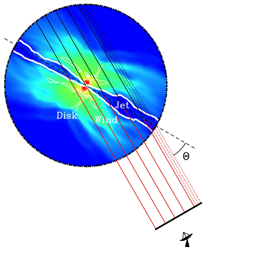
Figure 1: Schematic representation of the relevant portions of the simulated jet-wind-disk system and their relationship to example lines of sight. The thermal particle proper density is shown by the color map, extending over 9 orders of magnitude. The disk and jet regions are delineated by the thin and thick white lines, respectively. In between is the corona and wind (including both bound and unbound components). The limited extent of the disk and wind is due both to finite initial extent of the disk and to rotational collimation. The observer is shown in the lower-right, with the image plane immediately above. Lines of sight along which the ${\rm RM}$ and flux are integrated are shown, with the former being integrated along only the red portion. Dotted lines of sight pass through the initial transient portion of the simulation and are thus discarded (see Section 2.5). Finally, the definition of $\Theta$ is presented explicitly.

Provided the thermal electron temperature, proper density, four-velocity and magnetic field strength and geometry, we can now compute the ${\rm RM}$ along any given line of sight. Following Broderick & Loeb (2009), we do this directly via

$${\rm RM}=0.812\times 10^{6}\int\frac{f(T)n}{g^{2}}\left(\mbox{\boldmath$\rm\hat{k}$}-\mbox{\boldmath$\rm\beta$}\right)\cdot\mbox{\boldmath$\rm b$}d\ell\,{\rm rad}\,{\rm m}^{-2}\,,$$ (6)

where $g\equiv\Gamma\left(1-\mbox{\boldmath$\rm\beta$}\cdot\mbox{\boldmath$\rm\hat{k}$}\right)$ and we have supplemented this with a finite temperature term, given by,

$$f(T)=\frac{1}{\gamma^{2}}+\frac{\gamma-1}{2\gamma^{3}}\log\left(\gamma\right)\quad\text{where}\quad\gamma=\max\left(1,\frac{kT}{m_{e}c^{2}}\right)\,,$$ (7)

where $\gamma$ is the thermal particle Lorentz factor, not to be confused with the bulk Lorentz factor of the out-flowing gas (Huang et al., 2008; Shcherbakov, 2008). Note that the ${\rm RM}$, as we have defined it, depends solely upon quantities that have been simulated, with the integration geometry shown in Figure 1. All integrals are performed in flat space, ignoring any contributions from gravitational lensing, an approximation that is well-justified at the distances responsible for the resolved polarized emission. With this restriction, Equation (6) is correct for relativistically moving Faraday screens.

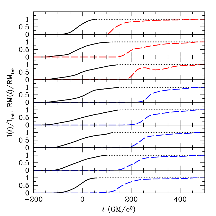
Figure 2: Fractional integrated intensity (black) and rotation measure (red & blue dashed lines, corresponding to positive and negative ${\rm RM}$s) as a function of distance as measured from the jet mid-plane along a number of exemplar lines of sight, which were chosen such that they span the width of the jet. After reaching 99% of its final value, the intensity is shown by a dotted line. In all cases, along any given line of sight the region responsible for the ${\rm RM}$ is well-separated from that responsible for producing the observed emission.

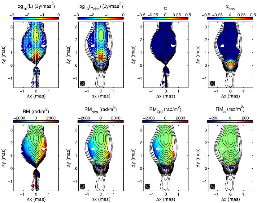
Figure 3: Ideal-resolution and beam-convolved polarized flux with unrotated polarization ticks (upper-left), spectral index (upper-right) and ${\rm RM}$ maps (lower-left) for our canonical jet model as observed at $15\,{\rm GHz}$ (see Table 3 for a complete list of relevant parameters). In addition the contributions from the two terms in Equation (21) are shown explicitly (lower-right). In all panels total flux contours are overlaid, in logarithmic factors of 2, with the minimum contour corresponding to $0.98\,{\rm m}{\rm Jy}{\rm mas}^{-2}$, and all other quantities are clipped at a polarized flux of $1\,{\rm m}{\rm Jy}\,{\rm mas}^{-2}$. Beam-convolved maps show the beam size ($0.3\,{\rm mas}$ FWHM) in their lower-left corner.

The integral in Equation (6) is performed from a vertical mid-plane, to a distant image plane, orthogonal to the line of sight. In principle, this overestimates the observed ${\rm RM}$ because it ignores depolarization along the line of sight resulting from Faraday rotation within the emitting region. However, in practice the emitting and rotating regions are well-separated, as illustrated explicitly in Figure 2, which shows the fractional local contributions to the Faraday rotation and emission (see the following section) along a representative line of sight. That this is the case is also supported directly by the observation of significant jet polarization fractions, ruling out substantial Faraday rotation within the emitting region (Burn, 1966; Gardner & Whiteoak, 1966). To generate an ${\rm RM}$ map, we then repeat this process many times at different positions on a rectilinear grid located on the image plane. Examples of the resulting maps can be found in Figure 3 and Section 3.

2.3 Jet Synchrotron Emission

While we may now compute the ${\rm RM}$ along any line of sight, given a complete description of the circum-jet material, in practice ${\rm RM}$s can be measured only for those lines of sight along which the jet is sufficiently bright. As a consequence, in order to compare with observations of AGN jets, we must also model the jet emission. This will serve two purposes: first as a mask upon the ${\rm RM}$-maps, identifying the regions that are observable, and second as a weight for determining the beam-convolved ${\rm RM}$ maps, as described in Section 2.4.

2.3.1 Particle Acceleration

Arising from nonthermal synchrotron emission within the jet itself, the emission is much more poorly constrained by the simulations. The difficult arises primarily from the lack of an ab initio understanding of the mechanism by which the radiating nonthermal electrons are accelerated. Here we consider a simple, qualitative model, appropriate when the accelerated electrons are the result of the dissipation of MHD turbulence and/or magnetic reconnection within the highly-magnetized jet. In this case the reservoir of energy that is available to be tapped via particle acceleration is that associated with the electromagnetic field. Thus, we set the comoving energy density in nonthermal electrons, $u_{\rm nth}$, proportional to that of the simulation electromagnetic field, $b^{2}/8\pi$. This assumption is consistent with minimum energy arguments used to infer the expected density of emitting particles and magnetic field strengths for emission due to synchrotron emission within AGNs (Burbidge, 1956). We further restrict the particle acceleration by requiring that it occur only in magnetically dominated regions, i.e., where $b^{2}/8\pi>\rho c^{2}$, which ensures that particles can be efficiently accelerated to large Lorentz factors via MHD turbulence and/or magnetic reconnection (Lyubarsky, 2005; Lyutikov, 2006). That is, explicitly, we set

$$u_{\rm nth}=\eta\frac{b^{2}}{4\pi}\left[1+\exp\left(\frac{\rho c^{2}}{b^{2}/8\pi}\right)\right]^{-1}\,,$$ (8)

and $\eta$ is the efficiency with which magnetic energy is converted into that in nonthermal particles [recall that $b^{2}\equiv\left|\mbox{\boldmath$\rm b$}\right|^{2}-\left(\mbox{\boldmath$\rm b$}\cdot\mbox{\boldmath$\rm\beta$}\right)^{2}$]. In magnetically dominated regions this reduces to $u_{\rm nth}=\eta b^{2}/8\pi$, and is exponentially suppressed otherwise. This is motivated first by the physical assumption that conversion of electromagnetic energy into nonthermal particles is less efficient when the electromagnetic energy per particle is low (e.g., relativistic magnetic reconnection requires, roughly, $b^{2}/(8\pi)\gg\rho c^{2}$, Lyutikov & Uzdensky, 2003). However, in practice relaxing this suppression results is broad flux distributions that are inconsistent with observations of AGN jets.

As a physically motivated alternative, one might choose $u_{\rm nth}$ to be proportional to the square of the comoving current density, indicative of where current sheets are dissipating (Lyutikov et al., 2005). However, the current density in the simulations is unlikely to be properly resolved and outside the current sheet the properties of the current layer are determined by the comoving electromagnetic energy density, suggesting that $u_{\rm nth}\propto b^{2}$ also roughly tracks the importance of current sheets if they were present. We leave the consideration of other prescriptions for the nonthermal particle density for future work.

We further assume a power-law electron distribution, with index $-2$ (resulting in a spectral index of 0.5) and minimum particle Lorentz factor, $\gamma_{\rm min}$, of $10^{2}$. Since our primary concern is to identify bright and dim regions, moderate changes in either of these do not significantly change our results.

2.3.2 Polarized Radiative Transfer in Bulk Flows

Due to the strong magnetic field within the jet and the relatively low density, the jet emission will be dominated by synchrotron. On ${\rm pc}$ scales, AGN jets are generally optically thin, while the bright radio core is optically thick. Thus, synchrotron self-absorption is critical to obtaining total jet fluxes and modelling the jet spectral index distribution. Furthermore, in order to compute the beam-convolved ${\rm RM}$s we will need intrinsic Stokes $I$, $Q_{0}$ and $U_{0}$. Thus we are necessarily faced with computing the self-absorbed, polarized emission.

The transfer of polarized radiation through relativistic environments has been discussed by a variety of authors and thus here we only summarize the procedure (see, e.g., Lindquist, 1966; Connors & Stark, 1977; Connors et al., 1980; Laor et al., 1990; Jaroszynski & Kurpiewski, 1997; Bromley et al., 2001; Broderick & Blandford, 2004; Beckwith & Done, 2005; Broderick, 2006; Broderick & Loeb, 2006). This is simplified somewhat by the assumption that within the regions of interest we may approximate the spacetime as being flat, requiring only that we consider the relativistic motion of the emission region. This results in the Doppler boosting and beaming of the emission as well as relativistic aberration of the polarization. All of these can be taken into account by noting that the photon occupancy numbers, $\propto(I,Q_{0},U_{0})/\nu^{3}$, are Lorentz scalars, allowing us to rewrite the standard radiative transfer equation in the emitting frame. From this we obtain,

$$\frac{d}{d\ell}\left(\begin{aligned} I\\ Q_{0}\\ U_{0}\end{aligned}\right)=\bar{j}_{\nu}\left(\begin{aligned} 1\\ \epsilon_{Q}\\ \epsilon_{U}\end{aligned}\right)-\bar{\alpha}_{\nu}\left(\begin{aligned} 1&&\zeta_{Q}&&\zeta_{U}\\ \zeta_{Q}&&1&&0\\ \zeta_{U}&&0&&1\\ \end{aligned}\right)\left(\begin{aligned} I\\ Q\\ U\end{aligned}\right)\,,$$ (9)

where $\bar{j}_{\nu}\equiv j_{g\nu}/g^{2}$ and $\bar{\alpha}_{\nu}\equiv g\alpha_{g\nu}$ are Lorentz covariant analogs of the lab-frame emission and absorption coefficients ($j_{\nu}$ and $\alpha_{\nu}$, respectively), which with $\epsilon_{Q,U}$ and $\zeta_{Q,U}$, are discussed in more detail below.

Generally, the form of $\bar{j}_{\nu}$ depends upon the locations of the minimum and maximum nonthermal particle Lorentz factors (we have specified only the former), and the location of a cooling break (located where particle acceleration balances synchrotron cooling). However, the cooling time at radio wavelengths exceeds the jet propagation time at ${\rm pc}$ scales, and thus we may safely ignore cooling in the computation of the ${\rm pc}$-scale radio images. Furthermore, while the maximum particle Lorentz factor generally depends upon the details of the particle acceleration mechanism, typical estimates, given the jet magnetic field strength, are much larger than the Lorentz factors of the particles responsible for the radio emission. This leaves the spectral break associated with $\gamma_{\rm min}$, giving

$$\bar{j}_{\nu}=C_{j}\frac{u_{\rm nth}}{g^{2}\gamma_{\rm min}}\nu_{B}\sin^{1.5}\vartheta\\ \times\left\{\begin{aligned} &\left(\frac{\nu_{B}}{g\nu_{\min}}\right)^{0.5}\left(\frac{\nu}{\nu_{\min}}\right)^{1/3}&&\text{if~{}}\nu<\nu_{\min}\\ &\left(\frac{\nu_{B}}{g\nu}\right)^{0.5}&&\text{otherwise,}\\ \end{aligned}\right.$$ (10)

in which $C_{j}\simeq 60\,{\rm Jy}\,{\rm c}{\rm m}^{2}\,{\rm erg}^{-1}\,{\rm Hz}^{-1}\,{\rm sr}^{-1}$, $\nu_{B}\equiv eb/2\pi m_{e}c$ is the cyclotron frequency in the comoving frame, $\sin\vartheta\equiv\sqrt{g^{2}b^{2}-\left[\left(\mbox{\boldmath$\rm\hat{k}$}-\mbox{\boldmath$\rm\beta$}\right)\cdot\mbox{\boldmath$\rm b$}\right]^{2}}\Big{/}gb$ is the sine of the angle between the line of sight and the magnetic field in the comoving frame, and $\nu_{\min}\equiv\gamma_{\rm min}^{2}\nu_{B}\sin\vartheta/g$ is the frequency associated with spectral break due to $\gamma_{\rm min}$. Given $\bar{j}_{\nu}$, we may determine $\bar{\alpha}_{\nu}$ via Kirchhoff’s law, giving,

$$\bar{\alpha}_{\nu}=C_{\alpha}g\frac{u_{\rm nth}}{\gamma_{\rm min}}\frac{\sin^{2}\vartheta}{\nu_{B}}\\ \times\left\{\begin{aligned} &\left(\frac{\nu_{B}}{g\nu_{\min}}\right)^{3}\left(\frac{\nu}{\nu_{\min}}\right)^{1/3}&&\text{if~{}}\nu<\nu_{\min}\\ &\left(\frac{\nu_{B}}{g\nu}\right)^{3}&&\text{otherwise,}\\ \end{aligned}\right.$$ (11)

where $C_{\alpha}\simeq 1.3\times 10^{6}\,{\rm c}{\rm m}^{-1}$.

The polarization terms are affected by both the relativistic aberration associated with the bulk motion of the jet and the orientation of the magnetic field. Both of these can be addressed by parallely propagating an orthonormal tetrad along the ray trajectory, defined at the image plane such that two of the basis vectors are aligned with the directions defining the observed Stokes parameters (and thus orthogonal to the line of sight). In principle, this basis may then be boosted into the emitting frame, directly accounting for relativistic aberration, and then compared with the projected direction of the magnetic field. In practice, it is sufficient to define the angle, $\xi$, between the initially vertical basis vector (associated with $Q$) and the projected magnetic field direction, in the emitting frame. As shown in Appendix A, this is defined up to a sign by

$$\cos\xi=\frac{\mbox{\boldmath$\rm\hat{z}$}\cdot\left(\mbox{\boldmath$\rm 1$}-\mbox{\boldmath$\rm\hat{k}$}\mbox{\boldmath$\rm\hat{k}$}\right)\cdot\left(\mbox{\boldmath$\rm b$}+\Gamma\mbox{\boldmath$\rm\beta$}b\cos\vartheta\right)}{\sqrt{1-\left(\mbox{\boldmath$\rm\hat{z}$}\cdot\mbox{\boldmath$\rm\hat{k}$}\right)^{2}}b\sin\vartheta}\,.$$ (12)

The sign of $\xi$ may then be obtained by a similar construction obtaining $\sin\xi$ from the relationship between the initially horizontal basis vector and the projected magnetic field in the emitting frame. However, it is sufficient to note the direction of $\rm b$ in the lab frame since boosting preserves the ordering of vectors, e.g., if $\rm b$ is to the right of $\rm\hat{z}$ (as seen by looking down the line of sight) in the emitting frame, then it will be so in all frames. Thus, $\sin\xi={\rm sgn}\left[\mbox{\boldmath$\rm\hat{b}$}\cdot\left(\mbox{\boldmath$\rm\hat{z}$}\times\mbox{\boldmath$\rm\hat{k}$}\right)\right]\sqrt{1-\cos^{2}\xi}$. In terms of these, the polarization terms are given by

$$\begin{gathered}\epsilon_{Q}=-\frac{9}{13}\cos 2\xi\,,\quad\epsilon_{U}=-\frac{9}{13}\sin 2\xi\,,\\ \zeta_{Q}=-\frac{3}{4}\cos 2\xi\,,\quad\zeta_{U}=-\frac{3}{4}\sin 2\xi\,,\\ \end{gathered}$$ (13)

where the particular numerical coefficients are set by the choice of the electron spectrum index and the overall sign reflects the fact that in the emitting frame the polarization is orthogonal to the projected magnetic field.

As with the expression for the ${\rm RM}$, Equations (9–13) are Lorentz covariant. Equation (9) is integrated throughout the emitting region along a given line of sight ending upon the image plane. However in practice, the emission is limited to the jet and associated accretion disk. Again, this procedure is repeated at a number of points upon the image plane, producing an image of the jet itself. Upon choosing a black hole mass, $\dot{M}$, distance and beam size, we generate a normalized radio map of the polarized jet emission, examples of which may be found in Figure 3 and Section 3.

In the following section we will find that the spatial distribution of the spectral index of the polarized emission, $\alpha_{L}$, will be important in determining the observed ${\rm RM}$ maps. As a consequence, we also construct $\alpha_{L}\equiv-d\log\sqrt{Q_{0}^{2}+U_{0}^{2}}/d\log\nu$ and $\alpha\equiv-d\log I/{\rm d}\log\nu$ by differencing polarized emission maps at nearby frequencies. Both $\alpha_{L}$ and $\alpha$ (an example of which is shown in Figure 3) are generally core dominated with a size indicative of the accretion rate.

2.4 Beam Convolution

Radio maps of AGN jets are generally under-resolved, with the consequence that a great deal of the jet substructure is smoothed out by the radio beam. However, in the case of the ${\rm RM}$ maps, we must take some care since ${\rm RM}$ is not observed directly. In this section we describe how we perform an appropriate beam convolution operation on the ${\rm RM}$ maps. We begin with a general discussion regarding finite beamwidth ${\rm RM}$ maps, and then move onto the particulars of the scheme we utilize in this paper.

2.4.1 Finite Beamwidth ${\rm RM}$ Maps in General

It is possible to infer the beam-convolved ${\rm RM}$ maps without producing fully simulated observations, i.e., without explicitly producing polarized images of the jet at multiple wavelengths. This is done by careful considering what is, and is not, directly measured. In practice, the ${\rm RM}$ is a derived quantity, computed from directly measured Stokes parameters $Q$ and $U$. Along with $I$, these are limited by the effective telescope beam, with the observed map being related to the infinite-resolution values via a convolution:

$$\left<I\right>(\mbox{\boldmath$\rm\Omega$})=\int d\Omega\,B(\mbox{\boldmath$\rm\Omega$}^{\prime}-\mbox{\boldmath$\rm\Omega$})I(\mbox{\boldmath$\rm\Omega$}^{\prime})\,,$$ (14)

with similar relations for $Q$, $U$ and $V$, in which $B(\mbox{\boldmath$\rm\Omega$})$ is the beam profile (which we will ultimately take to be Gaussian). In contrast, since ${\rm RM}$ is non-linearly related to $Q$ and $U$, the relationship between the finite-beam and the ideal-resolution ${\rm RM}$s is not a simple convolution. Nevertheless, as we show below, it may be written as the combination of weighted convolutions.

The effect of an intervening Faraday screen is to rotate $Q$ into $U$ and vice versa:

$$Q =L\cos\left(2\Psi_{0}+2{\rm RM}\lambda^{2}\right)$$ (15)

$$U =L\sin\left(2\Psi_{0}+2{\rm RM}\lambda^{2}\right)\,,$$

where $L=\sqrt{Q_{0}^{2}+U_{0}^{2}}$ is the intrinsic (ideal-resolution) polarized flux, $Q_{0}=L\cos\left(2\Psi_{0}\right)$ and $U_{0}=L\sin\left(2\Psi_{0}\right)$. The observed $Q$ and $U$ are then

$$\left<Q\right> =\left<L\cos\left(2\Psi_{0}+2{\rm RM}\lambda^{2}\right)\right>$$ (16)

$$\left<U\right> =\left<L\sin\left(2\Psi_{0}+2{\rm RM}\lambda^{2}\right)\right>\,,$$

and is now explicitly dependent upon the spatial distribution of the ${\rm RM}$ and $\lambda$. The observed polarization angle is

$$\Psi_{\rm obs}=\frac{1}{2}\arctan\left(\frac{\left<U\right>}{\left<Q\right>}\right)\,.$$ (17)

This implies that the measured ${\rm RM}$ is then

$${\rm RM}_{\rm obs} \equiv\frac{d\Psi_{\rm obs}}{d\lambda^{2}}$$ (18)

$$=\frac{1}{2\left(\left<Q\right>^{2}+\left<U\right>^{2}\right)}\left(\left<Q\right>\frac{d\left<U\right>}{d\lambda^{2}}-\left<U\right>\frac{d\left<Q\right>}{d\lambda^{2}}\right)\,.$$

Ignoring the wavelength dependencies in the beam size (which are explicitly accounted for with match-resolution images, produced by convolving high-frequency images with the lowest frequency-interval beam) $d/d\lambda^{2}$ commutes with the beam convolution. Thus, with Equations (15),

$$\frac{d\left<Q\right>}{d\lambda^{2}}=\left<\frac{dQ}{d\lambda^{2}}\right>=\left<Q\frac{\alpha_{L}}{2\lambda^{2}}\right>-2\left<U{\rm RM}\right>\,,$$ (19)

where we have assumed that $\Psi_{0}$ is wave-length independent (i.e., Faraday rotation is the only frequency dependence in $\Psi$). Similarly,

$$\frac{d\left<U\right>}{d\lambda^{2}}=\left<\frac{dU}{d\lambda^{2}}\right>=\left<U\frac{\alpha_{L}}{2\lambda^{2}}\right>+2\left<Q{\rm RM}\right>\,.$$ (20)

As a consequence,

$${\rm RM}_{\rm obs} =\frac{\left<Q\right>\left<Q{\rm RM}\right>+\left<U\right>\left<U{\rm RM}\right>}{\left<Q\right>^{2}+\left<U\right>^{2}}$$ (21)

$$\qquad+\frac{\left<Q\right>\left<U\alpha_{L}\right>-\left<U\right>\left<Q\alpha_{L}\right>}{4\lambda^{2}\left(\left<Q\right>^{2}+\left<U\right>^{2}\right)}\,.$$

The first term corresponds to a weighted average of the ${\rm RM}$ across the beam. Unresolved correlations between the polarized flux and the ${\rm RM}$ can produce substantial discrepancies between the intrinsic and observed ${\rm RM}$s. At this point we can identify some of the important differences between observations of ${\rm RM}$s and the polarized fluxes. If the ${\rm RM}$ is fixed across the beam we have ${\rm RM}_{\rm obs}={\rm RM}$ trivially. This is true even if there are rapid variations in the intrinsic polarization. The converse is not true; order $2\pi/\lambda^{2}$ variations in ${\rm RM}$ across the beam results in the well-known Faraday beam depolarization. More important are correlated variations in the polarized intensity and the ${\rm RM}$. Since ${\rm RM}_{\rm obs}$ is a weighted average, clear large-scale structures in the ${\rm RM}$ can be obscured by the presence of beam-scale structure in $L$. Thus even a uniform ${\rm RM}$ gradient can appear non-uniform at the beam-scale when illuminated by a spatially variable source, and in particular near the radio core where all quantities are changing on scales small in comparison to the observing beam.

The second term is associated with spatial variations in the polarized spectral index, vanishing identically when $\alpha_{L}$ is constant. This is due to the potential for frequency dependent competition among unresolved regions with different intrinsic polarizations. Spatially varying spectral indices have been found in a number of sources. Most common are swings from $\alpha_{L}\simeq 1$–$0.5$ within the optically thick AGN core and settling to $\alpha_{L}\simeq-0.5$ at angular distances of more than $\sim 1\,{\rm mas}$, where the jet is optically thin, though cases where similar magnitude variations across the jet occur are known, presumably due to interactions with the AGN environment (O’Sullivan & Gabuzda, 2009b, a). For comparison with these we also compute the beam-convolved spectral index:

$$\alpha_{\rm obs} \equiv\frac{d\log\langle I\rangle}{d\log\lambda}=\frac{\langle I\alpha\rangle}{\langle I\rangle}\,.$$ (22)

Examples may be found in Figure 3 and Section 3.

2.4.2 Beam-Convolved ${\rm RM}$ Gradients

We will remark upon the implications of finite beams for the ${\rm RM}$-maps of AGN jets in detail in the following sections. However, a simple, qualitative example directly illustrates the importance of beam convolution upon the search for, and study of, transverse ${\rm RM}$ gradients within AGN jets. We will find that generally it is crucial to resolve the transverse structure in both the emission and the ${\rm RM}$ distribution in order to obtain accurate measurements of the true ${\rm RM}$s.

We briefly consider a uniformly polarized 1D, cylindrically symmetric jet with a Gaussian transverse flux profile with width $\sigma_{J}$, a circular Gaussian beam with width $\sigma_{B}$, and a linear ${\rm RM}$-profile. The typical magnitude of the ${\rm RM}$s under consideration is $10^{3}\,{\rm rad}\,{\rm m}^{-2}$, which at $15\,{\rm GHz}$ produces Faraday rotations of $\sim 0.4\,{\rm rad}$. For the present purpose this is sufficiently small that it may be safely neglected (though we have confirmed this via explicit computation). Thus, without loss of generality we may set,

$${\rm RM}={\rm RM}_{0}^{\prime}x\,,\quad B=\frac{{\rm e}^{-x^{2}/2\sigma_{B}^{2}}}{\sqrt{2\pi}\sigma_{B}}\,,\quad Q=\frac{{\rm e}^{-x^{2}/2\sigma_{J}^{2}}}{\sqrt{2\pi}\sigma_{J}}\,,$$ (23)

where we have rotated the axes defining the Stokes parameters to force $U$ to vanish. With these the various beam-convolved quantities may be computed analytically, giving

$$\langle Q\rangle(x) =\int_{-\infty}^{\infty}dyB(y-x)Q(y)=\frac{{\rm e}^{-x^{2}/2(\sigma_{J}^{2}+\sigma_{B}^{2})}}{\sqrt{2\pi(\sigma_{J}^{2}+\sigma_{B}^{2})}}$$ (24)

$$\langle Q{\rm RM}\rangle(x) =\int_{-\infty}^{\infty}dyB(y-x)Q(y){\rm RM}(y)=\frac{{\rm RM}_{0}^{\prime}x\sigma_{J}^{2}}{\sigma_{J}^{2}+\sigma_{B}^{2}}\langle Q\rangle(x)\,,$$

which then implies

$${\rm RM}_{\rm obs}={\rm RM}\frac{\sigma_{J}^{2}}{\sigma_{J}^{2}+\sigma_{B}^{2}}\,.$$ (25)

That is, for linear ${\rm RM}$ gradients, the beam-convolved ${\rm RM}$s are generally smaller than the true values, and is a relatively strong function of the ratio of jet width to beam size. As a consequence, when the transverse jet structure is not resolved, even apparently linear ${\rm RM}$ gradients will not be accurate measures of the true jet ${\rm RM}$s. We will find that Equation (25) will be useful in interpreting the significance of unresolved, but nevertheless robust, ${\rm RM}$ gradients.

2.4.3 Computing Beam-Convolved ${\rm RM}$ Maps in Practice

Where the gradients in ${\rm RM}$ are sufficiently high, the procedure by which we have computed the ${\rm RM}$, $(I,Q_{0},U_{0})$ and $\alpha_{L}$ maps fails to resolve the rapidly varying polarizations. That is, when the image grid scales (generally much smaller than the beam size) are $\Delta\Omega_{x}$ and $\Delta\Omega_{y}$, if $\Delta\Omega_{x}d{\rm RM}/d\Omega_{x}\gtrsim\pi$ or $\Delta\Omega_{y}d{\rm RM}/d\Omega_{y}\gtrsim\pi$, we must supplement the inferred $Q$ and $U$ maps with a sub-grid model. Since the grid scale is much smaller than the typical beam scale, we may assume that $B(\mbox{\boldmath$\rm\Omega$})$ is roughly constant over a single pixel, and thus the primary effect corresponds to a grid-scale analog of beam depolarization. In this case, it is straightforward to show that the effective polarization fraction is

$$m_{L}=m_{L,0}\,{\rm sinc}\left(\Delta\Omega_{x}\frac{d{\rm RM}}{d\Omega_{x}}\lambda^{2}\right){\rm sinc}\left(\Delta\Omega_{y}\frac{d{\rm RM}}{d\Omega_{y}}\lambda^{2}\right)\,.$$ (26)

Thus, the procedure for producing the a finite-beam ${\rm RM}$ map is to first compute the ideal resolution ${\rm RM}$, $(I,Q_{0},U_{0})$ and $\alpha_{L}$ maps, pixel-depolarize these maps using Equation (26), and perform the convolutions in Equation (21) assuming a Gaussian beam. Examples of the resulting ${\rm RM}$ maps are presented in Figure 3 and Section 3.

2.5 Geometric Limitations

There are necessarily geometric limitations upon the jet inclinations, $\Theta$, for which we can produce ${\rm RM}$ maps. For $\Theta$ less than the jet half-opening angle, $\sim 3^{\circ}$ at $R_{\max}$, we are looking down the jet directly. As a consequence, the resulting ${\rm RM}$s are indicative of initial transients in the simulation, and of the radio lobe in real systems. Thus, we restrict ourselves to $\Theta\geq 10^{\circ}$.

However, these transients combined with the finite simulation time constrain the angular size of the image region more generally. The projected length of the jet is roughly $L_{\rm proj}\simeq R_{\max}\sin\Theta$. Lines of sight which pass through regions more distant than this, shown by the dotted lines in Figure 1, are necessarily indicative of the initial transient period. Thus, we limit ourselves to lines of sight that pass through the non-transient portions of the jet, and therefore restrict the region on the image plane we ultimately consider. Since this constraint becomes more severe at small $\Theta$, becoming impossible to satisfy when $\Theta$ is equal to the half-opening angle of the jet, the credible portions of the ${\rm RM}$ maps are necessarily different sizes for different inclinations.

3 Jet ${\rm RM}$ Maps and their Implications

ccccccccccc Jet model parameters Figure & $\nu$ beama $\Theta$ $R_{\max}$ $M$ $\dot{M}$ $\eta$ $a_{u}$ $\varepsilon$ $F_{15\,{\rm GHz}}$
(${\rm GHz}$) (${\rm mas}$) ($R_{\rm sim}$) ($10^{8}M_{\odot}$) ($\dot{M}_{\rm Edd}$) (${\rm Jy}$) 3,4,6,7,10,12 & 15 0.3 $20^{\circ}$ $10^{3}$ 3 0.01 0.02 $-8/3$ – 3.83
5,12 15 0.3 $10^{\circ}$ $10^{3}$ 3 0.005 0.02 $-8/3$ – 3.77
5,12 15 0.3 $30^{\circ}$ $10^{3}$ 3 0.018 0.02 $-8/3$ – 3.89
6 15 0.3 $20^{\circ}$ $10^{2}$ 30 $10^{-3}$ 0.02 $-8/3$ – 4.00
6,12 15 0.3 $20^{\circ}$ $10$ 300 $10^{-4}$ 0.02 $-8/3$ – 6.67
6 15 0.3 $20^{\circ}$ $1$ 3000 $10^{-5}$ 0.02 $-8/3$ – 12.7
7,12 15 0.3 $20^{\circ}$ $10^{3}$ 3 0.01 0.02 $-1.3$ 1 3.83
7 15 0.3 $20^{\circ}$ $10^{3}$ 3 0.01 0.02 $-1.3$ 0.1 3.83
7 15 0.3 $20^{\circ}$ $10^{3}$ 3 0.01 0.02 $-1.3$ 0.01 3.83
9 5 0.3 $20^{\circ}$ $10^{3}$ 3 0.01 0.02 $-8/3$ – 3.35
9 8 0.3 $20^{\circ}$ $10^{3}$ 3 0.01 0.02 $-8/3$ – 3.57
9 22 0.3 $20^{\circ}$ $10^{3}$ 3 0.01 0.02 $-8/3$ – 3.97
9,12 43 0.3 $20^{\circ}$ $10^{3}$ 3 0.01 0.02 $-8/3$ – 4.15
8 15 0.04 $20^{\circ}$ $10^{3}$ 3 0.01 0.02 $-8/3$ – 3.83
8 15 0.1 $20^{\circ}$ $10^{3}$ 3 0.01 0.02 $-8/3$ – 3.83
8,12 15 0.9 $20^{\circ}$ $10^{3}$ 3 0.01 0.02 $-8/3$ – 3.83 aFWHM

In this section we present ${\rm RM}$ maps for a variety of model, observational and theoretical parameters. These include variations in AGN model parameters (e.g., the jet orientation, black hole mass and magnetic dissipation rate; §3.1), observing parameters (observation frequency and beam size; §3.2) and the structure of the Faraday screen (§3.3). To ensure that we are comparing physically similar systems, we define a canonical model: A central black hole with mass $3\times 10^{8}M_{\odot}$ accreting at $1\%$ of the Eddington rate located at a distance of $300\,{\rm M}{\rm pc}$ and viewed at an inclination of $\Theta=20^{\circ}$. For the extrapolation we choose $R_{\max}=10^{3}R_{\rm sim}=10^{6}GM/c^{2}\simeq 15\,{\rm pc}$, and select $a_{u}=-8/3$, corresponding to the adiabatic advection model. Finally we choose $\eta=0.02$ such that the jet flux is roughly $4\,{\rm Jy}$ at $15\,{\rm GHz}$. These choices are not unique, and we will consider explicit departures from this canonical model in all respects; a list of the parameters of the models we present are listed in Table 3.

Figure 3 illustrates the general morphologies of the flux, polarization, spectral index and ${\rm RM}$ associated with our simulated jets. As in all subsequent ${\rm RM}$ maps, we show the polarization properties only where they are likely to be observed, requiring the polarized flux exceed $1\,{\rm m}{\rm Jy}\,{\rm mas}^{-2}$ . Specifically, in all cases we see an optically thick, small core that dominates the total and polarized emission (see the left-most and right-center upper panels). The ordered magnetic field within the jet results in an ordered polarization orientation, departing from the preferred direction only near the jet edge due to aberration and projection effects. Similarly, the ordered magnetic field in the material surrounding the jet results in an strongly-ordered ${\rm RM}$-map, exhibiting nearly linear transverse gradients along the length of the jet, and peaking near the core (lower-left panel).

These features, however, are somewhat obscured upon convolving with an observing beam. While generally the optically thick core is unresolved, it dominates the spectral index within a beamwidth of the core. The large ${\rm RM}$s near the core result in substantial beam depolarization, shifting the peak polarized flux away from the peak total flux. While the derotated polarization vectors retain their order, the polarization map can be dramatically effected, exhibiting the nearly linear gradients only when located more than a beamwidth from the core. This is primarily due to the first term in Equation (21), with the second term typically making $\sim 10\%$ corrections. While this suggests that the spectral index terms may be ignored, it should be noted that they produce gradients in random directions, and therefore directly obscure the transverse gradients indicative of the ordered toroidal magnetic fields.

3.1 Dependence of the ${\rm RM}$ upon the AGN Parameters

Here we address the importance of the jet and black hole parameters upon the ${\rm RM}$ maps. These arise via a number of the facets of our jet model, depending upon both the fundamental properties of the AGN itself as well as the assumptions that enter into the extrapolation scheme.

3.1.1 Jet Orientation

Chief among the jet properties affecting both the ${\rm RM}$ maps and the emission is the orientation. Having a self-consistent 3D-jet model provides the unique opportunity to assess the systematic uncertainty associated with non-axisymmetric jet structures, providing a fundamental lower limit upon the uncertainty associated with efforts to infer information about the circum-jet material from ${\rm RM}$ distributions.

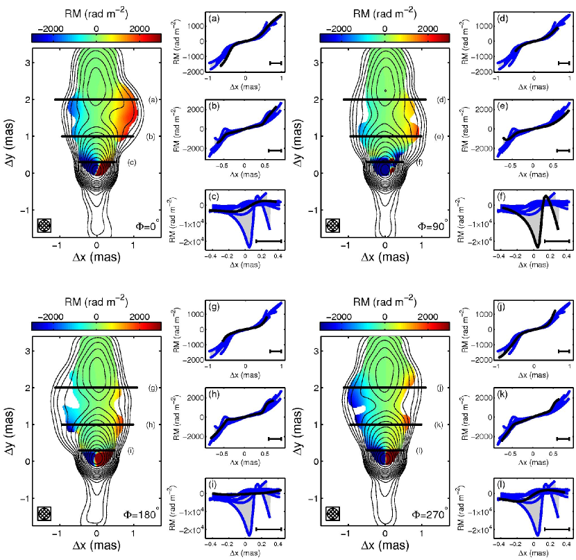
Figure 4: ${\rm RM}$ maps at $15\,{\rm GHz}$ for our canonical model (see Table 3 for a complete list of relevant parameters), as seen from a number of azimuthal angles, $\Phi$ (listed in the lower-right of each ${\rm RM}$ map). For reference total flux contours are overlayed, in logarithmic factors of 2, with the minimum contour corresponding to $0.98\,{\rm m}{\rm Jy}\,{\rm mas}^{-2}$. ${\rm RM}$s are shown only where the polarized flux exceeds $1{\rm m}{\rm Jy}\,{\rm mas}^{-2}$. Transverse profiles, corresponding to the labeled black bars, are shown to the right of each ${\rm RM}$ map (note the differences in the angular ranges). In addition to the ${\rm RM}$ profile for the view shown in each map (black), those from views with $\Phi=0^{\circ}$, $45^{\circ}$, $90^{\circ}$, $135^{\circ}$, $180^{\circ}$, $225^{\circ}$, $270^{\circ}$ and $315^{\circ}$ are shown in blue for comparison (with the enclosed envelope shown in grey). In all maps and transverse sections the beam size is shown in the lower-left and lower-right, respectively.

Figure 4 shows the ${\rm RM}$ maps for our canonical jet model as viewed from a variety of azimuthal angles, $\Phi$ (though all at the identical inclinations). To the right of each ${\rm RM}$ map we show example transverse profiles, taken near the core, far from the core and at an intermediate location. Within these the transverse profiles for views with $\Phi=0^{\circ}$, $45^{\circ}$, $90^{\circ}$, $135^{\circ}$, $180^{\circ}$, $225^{\circ}$, $270^{\circ}$ and $315^{\circ}$ are shown in addition to that associated with the neighboring map, providing a sense of the variations along each transverse section. Large variations among views indicates large inherent uncertainties in the ${\rm RM}$ values and their gradients due to the 3D jet structure.

Qualitatively, all azimuthal views are similar, exhibiting substantial beam depolarization in the radio core, and a region of large ${\rm RM}$s near the polarized flux maximum. Despite being nearly linear at all locations shown prior to beam convolution, where the transverse jet structure is not resolved the ${\rm RM}$ profiles vary significantly. However, despite the large structural variations in the jet itself, at positions further than a single beam, the transverse gradients become much more robust and are indicative of those present at ideal resolution.

Note that while the presence of substantial variations between transverse ${\rm RM}$ profiles does directly imply large uncertainties in the ${\rm RM}$ gradients, the inverse is not true. That is, consistent ${\rm RM}$ gradients do not necessarily imply that these are indicative of the circum-jet structure. As implied by Equation (25) and as we shall see explicitly below, it is possible for large beams to artificially produce essentially linear gradients that are considerably smaller than the associated intrinsic values.

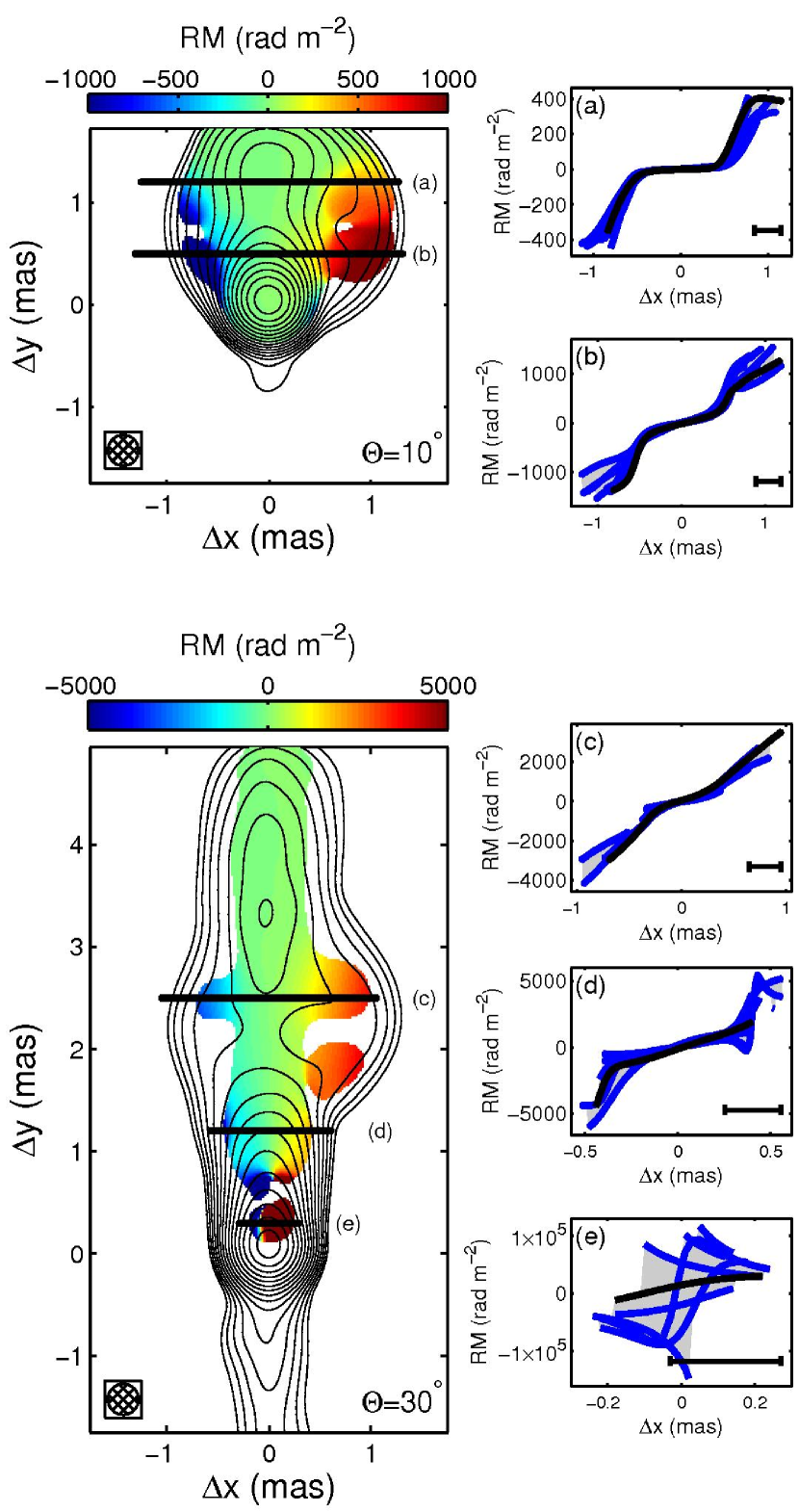
Figure 5: ${\rm RM}$ maps at $15\,{\rm GHz}$ for jets viewed at inclinations of $10^{\circ}$ (top) and $30^{\circ}$ (bottom; cf.the upper-left panels of Figure 4; see Table 3 for a complete list of relevant parameters). For reference total flux contours are overlayed, in logarithmic factors of 2, with the minimum contour corresponding to $0.98\,{\rm m}{\rm Jy}\,{\rm mas}^{-2}$. ${\rm RM}$s are shown only where the polarized flux exceeds $1{\rm m}{\rm Jy}\,{\rm mas}^{-2}$. To the right of each ${\rm RM}$ map, illustrative transverse ${\rm RM}$-profiles, corresponding to the labeled bars are shown (black) along with those from a variety of azimuthal viewing angles (blue). In all maps and transverse sections the beam size is shown in the lower-left and lower-right, respectively.

Jet inclination is known to have dramatic consequences for the appearance of AGN jets. This is also true for jet ${\rm RM}$-maps. Generally, where the emission becomes increasingly core dominated the finite beam effects (see Section 3.2) are exacerbated. In addition, at different jet inclinations the ${\rm RM}$s probe different circum-jet regions, with smaller $\Theta$ being sensitive to larger radii.

In Figure 5 we show the jets with inclinations of $\Theta=10^{\circ}$ and $30^{\circ}$. In order to ensure we are comparing observationally similar systems, we adjust the accretion rate so that the total flux is comparable to our canonical model, requiring variations of a factor of two in each direction (see Table 3). With this constraint, the ${\rm RM}$s are typically smaller at smaller inclinations, typically resulting in less depolarization. Indeed, at $\Theta=10^{\circ}$ the radio core is not depolarized, though finite beam effects do washout the ${\rm RM}$ gradients at this location. As with our canonical model, beyond a single beam width the transverse ${\rm RM}$ profiles become indicative of the ordered, ideal resolution values.

At larger inclinations the typical ${\rm RM}$s increase. As in the canonical case, the transverse ${\rm RM}$ profiles across the polarized flux core exhibit large variations among azimuthal viewing angles, and are thus unreliable measures of the circum-jet material. Less obvious is the fact that the intermediate transverse profile, Figure 5d, also fails to reproduce the ideal resolution ${\rm RM}$ gradients, despite the strong correlation between ${\rm RM}$ profiles obtained from differing azimuthal viewing directions. Based upon the simple model for beam-broadened ${\rm RM}$ gradients in Equation (25), we would anticipate a gradient roughly four times larger. Thus the substantially reduced values of the ${\rm RM}$ gradient cannot be accounted for simply due to the beam-broadened underlying ${\rm RM}$ gradients. Nevertheless, at sufficiently large distances, where the jet is resolved in the transverse direction, the ${\rm RM}$ gradients are reproduced with high fidelity, and the large-scale structure is clearly evident.

3.1.2 Black Hole Mass

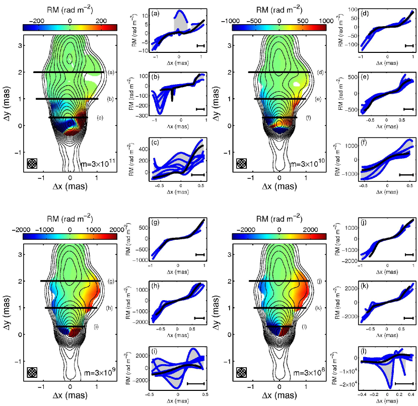
Figure 6: ${\rm RM}$ maps at $15\,{\rm GHz}$ for jets produced by black holes with a variety of masses ($m\equiv M/M_{\odot}$ is listed in the lower-right of each ${\rm RM}$ map; see Table 3 for a complete list of relevant parameters). Of particular note is the fact that at $3\times 10^{11}M_{\odot}$ no extrapolation is required. Our canonical model is shown in the lower-left. For reference total flux contours are overlayed, in logarithmic factors of 2, with the minimum contour corresponding to $0.98\,{\rm m}{\rm Jy}\,{\rm mas}^{-2}$. ${\rm RM}$s are shown only where the polarized flux exceeds $1{\rm m}{\rm Jy}\,{\rm mas}^{-2}$. To the right of each ${\rm RM}$ map, illustrative transverse ${\rm RM}$-profiles, corresponding to the labeled bars are shown (black) along with those from a variety of azimuthal viewing angles (blue). In all maps and transverse sections the beam size is shown in the lower-left and lower-right, respectively.

Variations in the black hole mass serve both to assess the importance of the intrinsic astrophysical variation in the masses of AGNs as well as the effects of our extrapolation scheme (Section 2.1.1). Here we choose to keep the physical size of the region of interest fixed, and therefore change $R_{\max}/R_{\rm sim}\propto M^{-1}$, i.e., change the degree of extrapolation. Since in all cases we are looking at the same underlying jet structure, we are necessarily gauging the relative importance of the black hole mass, or more specifically the length scale it provides.

Again we must address the problem of constructing observationally comparable systems. This is complicated by the fact that $m\equiv M/M_{\odot}=3\times 10^{11}$ systems, the mass required to avoid any extrapolation given the physical size ($15\,{\rm pc}$) and distance ($300\,{\rm M}{\rm pc}$) under consideration, are physically unrealistic. In principle, as in Figure 5 we would like to set $\dot{M}$ such that the total fluxes are comparable. However, this suggests the natural choice of fixed $\dot{M}$, or $\dot{M}/\dot{M}_{\rm Edd}\propto M^{-1}$, which is what we choose. If the emission were optically thin everywhere this would give the desired result. In practice the total flux varies by a factor of 3 over variations in mass over 3 orders of magnitude, ostensibly due to the subtlety different magnetic field geometry (see below). We might also expect the ${\rm RM}$s to be comparable: with $n\propto\dot{M}/r^{2}$ and $B\propto\left.n\right|_{r=M}^{1/2}(M/r)\propto\dot{M}^{1/2}/r$ we have ${\rm RM}\sim nBr\propto\dot{M}^{3/2}/r^{3}$ and thus at fixed $r$, ${\rm RM}\sim\dot{M}^{3/2}$. This is not, however, the case, with the typical ${\rm RM}$s of less massive black holes being considerably larger than those of their larger analogs. Far from the radio core, where the beam convolved ${\rm RM}$s are indicative of the true values, we find that in practice ${\rm RM}\propto M^{-1}$ (though, for a given mass the ${\rm RM}$s do have the expected dependence upon accretion rate).

Near the black hole the toroidal and poloidal components of the magnetic field have similar magnitudes. Thus the results of Section 2.1.1 imply that at fixed physical distance $b^{P}/b^{\phi}\propto M$. Since outside the jet $\rm b^{P}$ undergoes stochastic variations, we may therefore expect to find less ordered ${\rm RM}$ profiles at larger masses, exhibiting more vertical structure. As seen in Figure 6, this is indeed the case. For $m\equiv M/M_{\odot}\gtrsim 3\times 10^{10}$ vertical gradients can begin to dominate the ${\rm RM}$ map near the core, extending further and becoming more prominent as $m$ increases. This vertical structure is an intrinsic effect, appearing in the ideal resolution ${\rm RM}$ maps as well. This is in contrast to ${\rm RM}$-gradient reversals near the core for $m\lesssim 3\times 10^{10}$, which are exclusively due to finite beam effects.

The transverse gradients near the radio core at lower masses are clearly not indicative of the true, nearly linear ${\rm RM}$ gradients. However, for $m\gtrsim 3\times 10^{10}$ the transverse ${\rm RM}$ profiles in Figure 6c & 6f are more robust, exhibiting a clearly identifiable gradients. While the ${\rm RM}$ gradients along the nearby sections are well below the true values, they are consistent with the beam-broadened values anticipated by Equation (25). Since in practice the jet width is not known a priori, determining the true gradients along these sections is not possible for AGN jets associated with the most massive black holes expected in nature. Nevertheless, in this case the presence of a robust gradient, even if unresolved, is indicative of ordered toroidal fields.

3.1.3 Magnetic Dissipation in the Faraday Screen

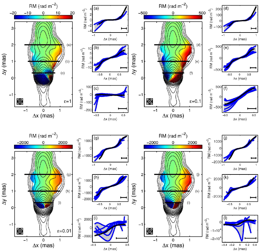
Figure 7: ${\rm RM}$ maps at $15\,{\rm GHz}$ for jets in which the jet sheath is efficiently heated via magnetic dissipation ($\varepsilon$ is listed in the lower-right of each ${\rm RM}$ map; see Table 3 for a complete list of relevant parameters). For each the internal energy is extrapolated using $a_{u}=-1.3$ until it reaches $\varepsilon b^{2}/8\pi$ (generally, this occurs quite close to the black hole). The upper-left, upper-right and lower-left panels correspond to $\varepsilon=1.0$, $0.1$ and $0.01$, respectively. For comparison the canonical model ($a_{u}=-8/3$) is shown in the lower-right panel. For reference total flux contours are overlayed, in logarithmic factors of 2, with the minimum contour corresponding to $0.98\,{\rm m}{\rm Jy}\,{\rm mas}^{-2}$. ${\rm RM}$s are shown only where the polarized flux exceeds $1{\rm m}{\rm Jy}\,{\rm mas}^{-2}$. To the right of each ${\rm RM}$ map, illustrative transverse ${\rm RM}$-profiles, corresponding to the labeled bars are shown (black) along with those from a variety of azimuthal viewing angles (blue). In all maps and transverse sections the beam size is shown in the lower-left and lower-right, respectively.

Finally, we consider the dependence of the ${\rm RM}$s upon the rate at which magnetic dissipation heats the circum-jet material. The transition from hot ($kT>m_{e}c^{2}$) gas within the jet to cool ($kT<m_{e}c^{2}$) gas surrounding the jet is typically rapid, occurring over less than a jet width. Nevertheless, since $f(T)$ is such a strong function of $kT/m_{e}c^{2}$ (see Equation (21)), the location of this transition can substantially affect the typical ${\rm RM}$s produced near the jet. Since $b^{2}/8\pi\rho c^{2}>1$ within the jet, efficient dissipation of magnetic energy in the jet sheath can easily heat the circum-jet material sufficient to suppress Faraday rotation.

This is explicitly seen in Figure 7, which shows the efficient heating model for a number of maximum heating rates $\varepsilon$ (recall, we set the maximum internal energy to $\varepsilon b^{2}/8\pi$). When $\varepsilon=1.0$ the typical ${\rm RM}$s are reduced by more than two orders of magnitude. In contrast, setting $\varepsilon\lesssim 0.01$ results in nearly identical values to those from our canonical model. In all cases, with the exception of regions near the core, the basic structure of the ${\rm RM}$ maps and their transverse profiles are qualitatively similar.

As for the canonical case (shown in the lower-right panel of Figure 7), where the transverse structure of the jet is resolved the ${\rm RM}$s are indicative of the true values. Similarly, the transverse profiles near the core are typically unreliable. An exception is the appearance of a robust gradient at this location when $\varepsilon=0.1$ (Figure 7f). In this case the resulting beam-convolved gradients are indeed consistent with those expected from Equation (25). In contrast, despite exhibiting a general trend, the ${\rm RM}$s in Figure 7i are roughly an order of magnitude lower than would be expected. As a result, it may be difficult to assess the fidelity of an observed transverse ${\rm RM}$ gradient when the jet width is insufficiently unresolved.

3.2 Dependence of the ${\rm RM}$ upon the Observation Parameters

In addition to the parameters of the AGN model, the measured ${\rm RM}$ can depend upon how they are observed as well. Here we address two ways in which this occurs: observing frequency and beam size. In order to isolate the effects of each, we treat them separately by fixing one while varying the other. All of these are essentially finite beam effects; in all cases shown in Figures 9 & 8 the intrinsic, ideal resolution ${\rm RM}$ maps are identical.

3.2.1 Beam Size

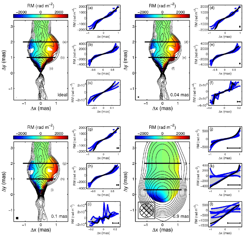
Figure 8: ${\rm RM}$ maps of our canonical model at $15\,{\rm GHz}$ as observed with a number of different beam sizes (beam FWHMs are listed in the lower-right of each ${\rm RM}$ map; cf. the upper-left panel of Figure 4; see Table 3 for a complete list of relevant parameters). In particular, we show the map at the computed pixel resolution ($0.02\,{\rm mas}$, upper-left), the highest design resolution of VSOP-2 ($0.04\,{\rm mas}$, upper-right), the highest typical VLBA resolution ($0.1\,{\rm mas}$, lower-left) and the typical VLBA resolution at $5\,{\rm GHz}$ ($0.9\,{\rm mas}$, lower-right). For reference total flux contours are overlayed, in logarithmic factors of 2, with the minimum contour corresponding to $0.98\,{\rm m}{\rm Jy}\,{\rm mas}^{-2}$. ${\rm RM}$s are shown only where the polarized flux exceeds $1{\rm m}{\rm Jy}\,{\rm mas}^{-2}$. To the right of each ${\rm RM}$ map, illustrative transverse ${\rm RM}$-profiles, corresponding to the labeled bars are shown (black) along with those from a variety of azimuthal viewing angles (blue). In all maps and transverse sections the beam size is shown in the lower-left and lower-right, respectively.

We have alluded to the importance of beam size a number of times already; generally finding that where the beam does not resolve the transverse structure of the jet the transverse ${\rm RM}$ profiles are inaccurate. Here and in Figure 8 we make these statements explicit by convolving the same image (corresponding to our canonical model; see Table 3 for details) with a number of different beams. These correspond to the highest typical VLBA resolution at $5\,{\rm GHz}$ ($0.9\,{\rm mas}$), highest typical VLBA resolution at $43\,{\rm GHz}$ ($0.1\,{\rm mas}$), highest design resolution for VLBI using the upcoming space-based radio telescope VSOP-2 ($43\,{\rm GHz}$, $0.04\,{\rm mas}$, Tsuboi et al. 2009) and the computational resolution ($\sim 0.02\,{\rm mas}$). These can also be compared with our canonical model (e.g. Figure 4), which has a beam typical of VLBA observations at $15\,{\rm GHz}$.

The $0.9\,{\rm mas}$ and $0.3\,{\rm mas}$ beams are typical of matched-resolution ${\rm RM}$ studies, and thus provide insight into the ability of the existing literature to constrain the parameters of simulated jets. VSOP-2 promises to achieve beam sizes of $\sim 0.1\,{\rm mas}$ at $8\,{\rm GHz}$, roughly a factor of two improvement over the VLBA. Thus, $0.1\,{\rm mas}$ beam is indicative of what may be possible in the near future. Finally, VSOP-2’s maximum resolution gives a lower-limit on realistically attainable beam widths over the next decade, though in this case the observed ${\rm RM}$s would be obtained only over a relatively small wavelength range.

As previously stated, the ideal resolution case produces clear, nearly linear transverse gradients along the length of the jet. VSOP-2  should be able to probe gradients as close as $0.3\,{\rm mas}$ to the radio core. Similarly, high frequency observations at the VLBA faithfully reproduce the transverse ${\rm RM}$ gradients in the optically thin region, though near the radio core large spurious fluctuations develop.

In contrast, for large beams, while apparently linear gradients exist, these are in some cases clearly anomalous, arising from the breadth of the beam instead of the structure of the jet. This is most clearly evident in the bottom two transverse profiles, Figure 8k & 8l, which show profiles with a number of different gradients, in some cases with the wrong sign. In Figure 8k, the presence of inverted gradients provides a strong case against interpreting these as due to the true structure in the ${\rm RM}$ map. However, the average profile in this case is roughly consistent (within 50%) with that anticipated by Equation (25). In contrast, Figure 8l exhibits ${\rm RM}$ gradients which are all of the correct sign, though also all well below the values expected even after accounting for the beam-broadening of the profiles. Far from the radio core, despite being unresolved, the transverse gradients are strongly correlated in azimuthal viewing angle and are well-described Equation (25), producing gradients roughly a factor of 4 smaller than the true values. Thus, despite the inability to infer the actual ${\rm RM}$ values due to the failure to resolve the jet transverse structure, the structure in the ${\rm RM}$ map is indeed indicative of the ideal-resolution ${\rm RM}$s more than a beam width from the radio core.

3.2.2 Frequency

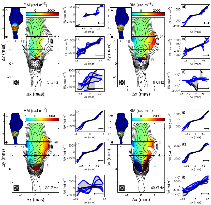
Figure 9: ${\rm RM}$ maps of our canonical model as observed $\nu=5\,GHz$, $8\,{\rm GHz}$, $22\,{\rm GHz}$ and $43\,{\rm GHz}$ (observation frequecies are listed in the lower-right of each ${\rm RM}$ map; cf. the upper-left panel of Figure 4; see Table 3 for particular parameters). In all cases the beam size is fixed to $0.3\,{\rm mas}$. The beam-convolved spectral index map is shown in the upper-left inset of each ${\rm RM}$ map, in which the colors range from $-0.5$ (dark blue) to $0.5$ (dark red), indicating the size of the photosphere at each frequency. For reference total flux contours are overlayed, in logarithmic factors of 2 (factors of 8 in the $\alpha$ map insets), with the minimum contour corresponding to $0.98\,{\rm m}{\rm Jy}\,{\rm mas}^{-2}$. ${\rm RM}$s are shown only where the polarized flux exceeds $1{\rm m}{\rm Jy}\,{\rm mas}^{-2}$. To the right of each ${\rm RM}$ map, illustrative transverse ${\rm RM}$-profiles, corresponding to the labeled bars are shown (black) along with those from a variety of azimuthal viewing angles (blue). In all maps and transverse sections the beam size is shown in the lower-left and lower-right, respectively.

While we have defined the ${\rm RM}$ in the differential sense, where the $\lambda^{2}$-law holds in the ideal-resolution ${\rm RM}$ maps, we might anticipate that frequency effects may be neglected. However, as seen in Figure 9 (cf. 4), near the radio core this is not the case generally. Despite having identical intrinsic ${\rm RM}$s, differences in the photosphere size and beam depolarization associated with different observing frequencies can dramatically alter the beam-convolved ${\rm RM}$ maps. Note that here we fix the beam size to $0.3\,{\rm mas}$ despite the change in observing frequency.

Firstly, the increase in beam depolarization at longer wavelengths severely restricts the region over which the ${\rm RM}$s may be measured. At $5\,{\rm GHz}$, the jet is a few beams across, and begins to suffer from inadequate transverse resolution. As a consequence, even where the jet is optically thin, the beam-convolved ${\rm RM}$ map exhibits substantial variations about the true values. The ${\rm RM}$ profile shown in Figure 9b is roughly a factor of two below the true values, though in agreement with those predicted by Equation (25). By $8\,{\rm GHz}$ the jet is sufficiently resolved (given our polarized flux limit of $1\,{\rm m}{\rm Jy}\,{\rm mas}^{-2}$) that the gradients in the optically thin portions of the jet (e.g. the top two transverse profiles) reproduce the true gradients with high fidelity.

Secondly, the size of the radio photosphere shrinks as frequency increases, with a corresponding decrease in the consequences of the rapid variations in the spectral index. At $5\,{\rm GHz}$ the photosphere extends roughly $0.5{\rm mas}$, larger than the beam itself, while at $43\,{\rm GHz}$ it is comparable to the resolution with which we computed the intrinsic ${\rm RM}$ maps ($0.02\,{\rm mas}$). The decrease in the importance of the optically thick core is seen most dramatically in the appearance of the consistent transverse gradients close to the core, Figure 9l, which are roughly an order of magnitude below the true values, consistent with Equation (25).

When the beam size is increased to $0.9\,{\rm mas}$ all of the profiles at $5\,{\rm GHz}$ fail to reproduce even the beam-broadened ${\rm RM}$ gradients. Nevertheless, above $8\,{\rm GHz}$, as in Figure 8j, transverse profiles far from the core exhibit robust gradients indicative of the expected values for transversely unresolved jets. This is also true at intermediate distances from the radio core (Figure 9h & 9k) for frequencies above $22\,{\rm GHz}$. Finally, at $43\,{\rm GHz}$, the highest frequency we consider, even the core ${\rm RM}$ profiles are well-defined and in agreement with the values anticipated by Equation (25), though roughly two order of magnitudes smaller than the true values. Thus, for the purposes of detecting robust ${\rm RM}$ gradients associated with poorly resolved structure within the Faraday screen, pushing to high frequencies alone can partially ameliorate resolution issues (though, as addressed explicitly in Section 3.4, it may be difficult to distinguish between nearby and distant Faraday screens in this case).

The differences between the ${\rm RM}$ maps near the radio core due to beam convolution necessarily implies that the $\lambda^{2}$-law is violated in this region. On the other hand, when the transverse jet structure is sufficiently resolved and the observed ${\rm RM}$s agree with the intrinsic ${\rm RM}$s, as occurs far from the core in the optically thin region, then similarities between the ${\rm RM}$s implies that the $\lambda^{2}$-law holds. These regions also differ in how well the beam-convolved ${\rm RM}$ maps reproduce the true values. Hence, this suggests that at least for our simulated AGN jets, the $\lambda^{2}$-law provides a rough measure of the accuracy of the ${\rm RM}$ gradients when the ${\rm RM}$s are sufficiently resolved.

3.3 Dependence of the ${\rm RM}$ upon the Jet Structure

The primary motivation for studying the ${\rm RM}$ distributions of AGN jets has been to infer the structure and parameters of the Faraday screen. In the context of the 3D simulation, neither of these are free parameters, and we have obtained a characteristic, bilateral structure for the ${\rm RM}$ maps, presumably as a consequence of large-scale structure within the Faraday screen. Here we address how these morphological features are related to the structural properties of the Faraday screen itself. We do this by artificially removing components of the magnetic field & velocity and recomputing the ${\rm RM}$ map, while using our canonical model to produce the jet emission.

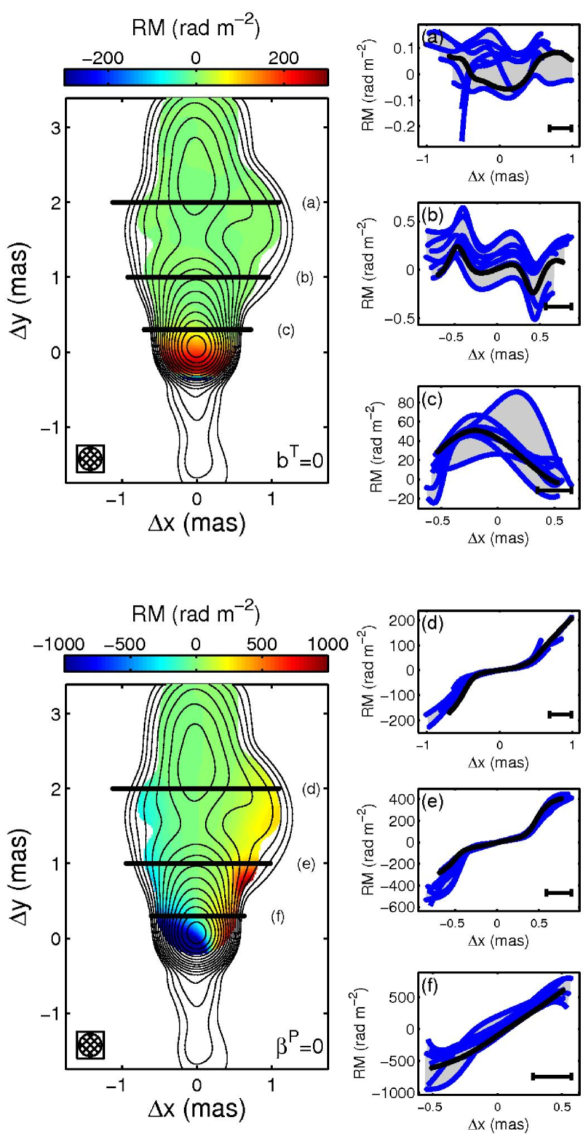
Figure 10: ${\rm RM}$ maps at $15\,{\rm GHz}$ when toroidal component of the comoving magnetic field (top) and poloidal component of the velocity (bottom) of the plasma within the Faraday screen is made to artificially vanish (cf. the upper-left panel of Figure 4; see Table 3 for a complete list of relevant parameters). For reference total flux contours are overlayed, in logarithmic factors of 2, with the minimum contour corresponding to $0.98\,{\rm m}{\rm Jy}\,{\rm mas}^{-2}$. ${\rm RM}$s are shown only where the polarized flux exceeds $1{\rm m}{\rm Jy}\,{\rm mas}^{-2}$. To the right of each ${\rm RM}$ map, illustrative transverse ${\rm RM}$-profiles, corresponding to the labeled bars are shown (black) along with those from a variety of azimuthal viewing angles (blue). In all maps and transverse sections the beam size is shown in the lower-left and lower-right, respectively.

3.3.1 Magnetic Field Structure

The relationship between the poloidal and toroidal magnetic field has already been indirectly demonstrated to have a significant effect upon the structure of the ${\rm RM}$ map. Large poloidal fields (e.g., those associated with $m=3\times 10^{11}$) can result in the loss of the transverse symmetry apparent outside of the radio core. This is illustrated explicitly in the top panel of Figure 10, which presents the ${\rm RM}$ map when the toroidal component of the magnetic field in our canonical model is artificially made to vanish. Significant transverse gradients vanish completely everywhere within the jet (where it is sufficiently resolved), confirming that nearly-linear, resolved transverse gradients are due to large-scale, ordered toroidal magnetic fields within the Faraday screen.

The remnant ${\rm RM}$ is that associated with the poloidal field, and is thus roughly 3 orders of magnitude smaller than that in our canonical model (see, Figure 4). This is a function of the black hole mass, with $b^{P}/b^{T}\propto M^{-1}$ at fixed physical distance, and thus the perturbations due to poloidal fields will be larger for more massive systems. Nevertheless, it appears that for typical blazars and BL Lac objects the fixed offset in the transverse profile due to the presence of poloidal fields will be dominated by the uncertainties in the location of the jet spine (not necessarily located along the jet axis), viewing angle and finite beam effects for single ${\rm RM}$ profiles. It remains to be seen if it is possible to reduce these uncertainties by combining multiple profiles, making use of the strong correlation in these quantities along the jet axis.

3.3.2 Velocity Structure

The large Lorentz factors within AGN jets suggest that the velocity structure of the Faraday screen may also be important. The degree to which this occurs in practice depends upon the location of the Faraday screen and how coupled it is to the jet itself.

Setting the poloidal velocity to vanish, shown in the bottom panel of Figure 10, made little difference to the overall morphology of the ${\rm RM}$ map. It does, however, decrease the typical ${\rm RM}$s by a factor of roughly 4. This is not unexpected if the typical Lorentz factors within the Faraday screen are on the order of 2 (a fact that will be borne out in the following section); from Equation (21),

$$\frac{\left.{\rm RM}\right|_{\beta^{P}=0}}{{\rm RM}}\simeq\Gamma^{2}\left(1-\beta^{P}\cos\Theta\right)^{2}\simeq\Gamma^{2}\left[\frac{1}{\Gamma^{2}}+\frac{\Theta^{2}}{2}\right]^{2}\,,$$ (27)

which when $\Theta\lesssim\sqrt{2}/\Gamma$ reduces to $\Gamma^{-2}$. Unlike the canonical case, when the poloidal velocity is made to vanish the transverse ${\rm RM}$ profiles exhibit a well-defined, nearly linear gradients near the core. These are roughly an order of magnitude smaller than the true ${\rm RM}$s, though in agreement with those expected by Equation (25).

In contrast, the toroidal velocities appear to have little effect beyond the radio core. This is not particularly surprising since from Section 2.1.1 we have that $\beta^{T}/\beta^{P}\sim\left(GM/c^{2}r\right)^{-1}$, and thus at the large distances (in terms of the gravitational radius of the black hole) seen here we anticipate the toroidal velocities to be roughly 5 orders of magnitude smaller than the poloidal values within the screen. Thus the kinds of effects associated with large-scale relativistic motions described in Broderick & Loeb (2009) are likely to be unimportant in the case of isolated, roughly stable jets.

3.4 Location and Structure of the Jet Faraday Screen

While we have described how some of the most commonly discussed features of the circum-jet environment imprint themselves upon the ${\rm RM}$ map, we have said little about the location and structure of the Faraday rotating medium. Here we address this, identifying what portion of the outflow is responsible for generating the Faraday rotation and how it is related to the jet itself. In addition, we address how this may be distinguished from non-local models of the Faraday screen.

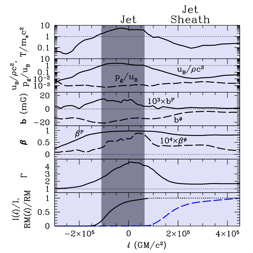
Figure 11: Plasma quantities along an example line of sight, in comparison to the location of the Faraday screen. The locations of the jet, defined by $\rho c^{2}<u_{B}\equiv b^{2}/8\pi$, and its surrounding sheath, defined by $p_{g}<u_{B}/3$, are represented by the dark and light gray shaded regions, respectively. This corresponds a line of sight responsible for producing the ${\rm RM}$ at an angular position of $\Delta\Omega_{x}=1\,{\rm mas}$ and $\Delta\Omega_{y}=1.5\,{\rm mas}$, and is the second from the bottom line of sight shown in Figure 2, with the intensity (solid black line) and rotation measure (dashed, blue line) shown explicitly in the bottom panel.

A number of relevant plasma quantities, in addition to $I_{\nu}$ and the ${\rm RM}$, along a representative line of sight are shown in Figure 11, including the poloidal and toroidal components of $\rm\beta$ and $\rm b$, the Lorentz factor and temperature. Generally, the Faraday screen is quite close to the jet, lying within two jet widths of the jet axis. The bulk of the Faraday rotation occurs within the strongly magnetized jet sheath, defined here by when the gas pressure is less than $1/3$ of the magnetic pressure (i.e., the plasma $\beta<1/3$), though at larger inclinations a significant fraction may occur within the surrounding wind. While the Faraday screen and emission region are well-separated, they are both parts of a larger MHD structure. As illustrated in Figure 11, the jet sheath is a smooth extension of the jet itself; i.e., there is no well-defined spine-sheath structure despite our identification of a jet “sheath” (cf. Laing & Bridle, 2002b, a).

The entire rotating region is unbound in the particle, thermal and magneto-thermal senses, i.e.,

$$\begin{gathered}-u_{t}\simeq\left(1-\frac{2GM}{c^{2}r}\right)\Gamma>1\,,\\ -hu_{t}\simeq\left(1-\frac{2GM}{c^{2}r}\right)\frac{\rho+u_{g}+p_{g}}{\rho}\Gamma>1\,,\\ -\frac{T^{P}_{t}}{\rho u^{P}}\simeq\left(1-\frac{2GM}{c^{2}r}\right)\frac{\left(\rho+u_{g}+p_{g}\right)\Gamma^{2}\beta^{P}-b^{P}\mbox{\boldmath$\rm\beta$}\cdot\mbox{\boldmath$\rm b$}}{\rho\Gamma\beta^{P}}>1\,,\end{gathered}$$ (28)

respectively, where $T^{P}_{t}$ is the contravariant poloidal, covariant time component of the ideal MHD stress-energy tensor, $u_{t}$ is the covariant time component of the 4-velocity, and $u^{P}$ is the contravariant poloidal component of the 4-velocity. Therefore, the Faraday screen is clearly associated with the large-scale outflow. Despite this, the Lorentz factor of the Faraday rotating material is generally much lower than the jet interior, $\Gamma\simeq 2$, due in part to the strong dependence upon $\Gamma$ of the integrand in Equation (6).

The ${\rm RM}$ is dominated by contributions close to the jet and not by the disk wind. In the simulations, the disk wind is not as well-collimated as the jet due to the finite extent of the accretion flow. While the highly relativistic jet becomes mostly ballistic when losing lateral support due to the finite disk extent, the weakly relativistic disk wind fills the space as a more spherical outflow. Even the part of the disk wind launched from near the black hole has a significant loss of toroidal field strength with radius compared to the relativistic jet due to the overall expansion of the disk wind. The simulations suggest that a disk extent of order ${\rm pc}$-scales may be required to have a well-collimated disk wind that significantly contributed to the ${\rm RM}$ on ${\rm pc}$-scales.

Throughout the duration of the 3D GRMHD simulation we have used, there is no evidence for the presence of reversed field polarity as in the “magnetic tower” picture discussed by Mahmud et al. (2009). They suggested that the time-dependent sign of the ${\rm RM}$ in BL Lac object B1803+784 can be explained best by magnetic tower models containing nested, reversed helical fields, in which the inner field changes (in time) its degree of winding relative to the outer return field. In the GRMHD simulations, at no point along the line of sight does the toroidal component of the comoving or lab-frame magnetic field reverse direction It appears unlikely that a significant fraction of the observed ${\rm RM}$ can be due to a distant, reversed region, as in a disk wind. Furthermore, such reversed magnetic tower geometries appear to be at odds with jets launched by accretion disks, for which the interior of the jet is universally more tightly wound due to the monotonically decreasing radial Keplerian rotation profile. One might be able to invoke a slowly rotating black hole connected to time-varying launching points in the Keplerian disk. However, this requires a slowly rotating black hole with $a/M\lesssim 0.4$, at which the total power of the disk wind may dominate that of the black hole jet (McKinney, 2005) leaving the emission dominated by a quasi-spherical region instead of a collimated jet. Sign changes could potentially be due to changes in the overall polarity of a dipolar field near the black hole, although this may be at odds with the long-term constancy of the sign of the ${\rm RM}$ gradient. On the other hand, the presence of instantaneous erroneous ${\rm RM}$ gradients (even sign changes) due to the finite beam size can produce qualitatively similar behaviors near the radio core, and might be responsible for the apparent time-dependence, though we should note that in B1803+784 the reversal occurred far from the radio core. An investigation of ${\rm RM}$s that considers these issues, such as considering ${\rm RM}$s from time-dependent simulations, is left for future work.

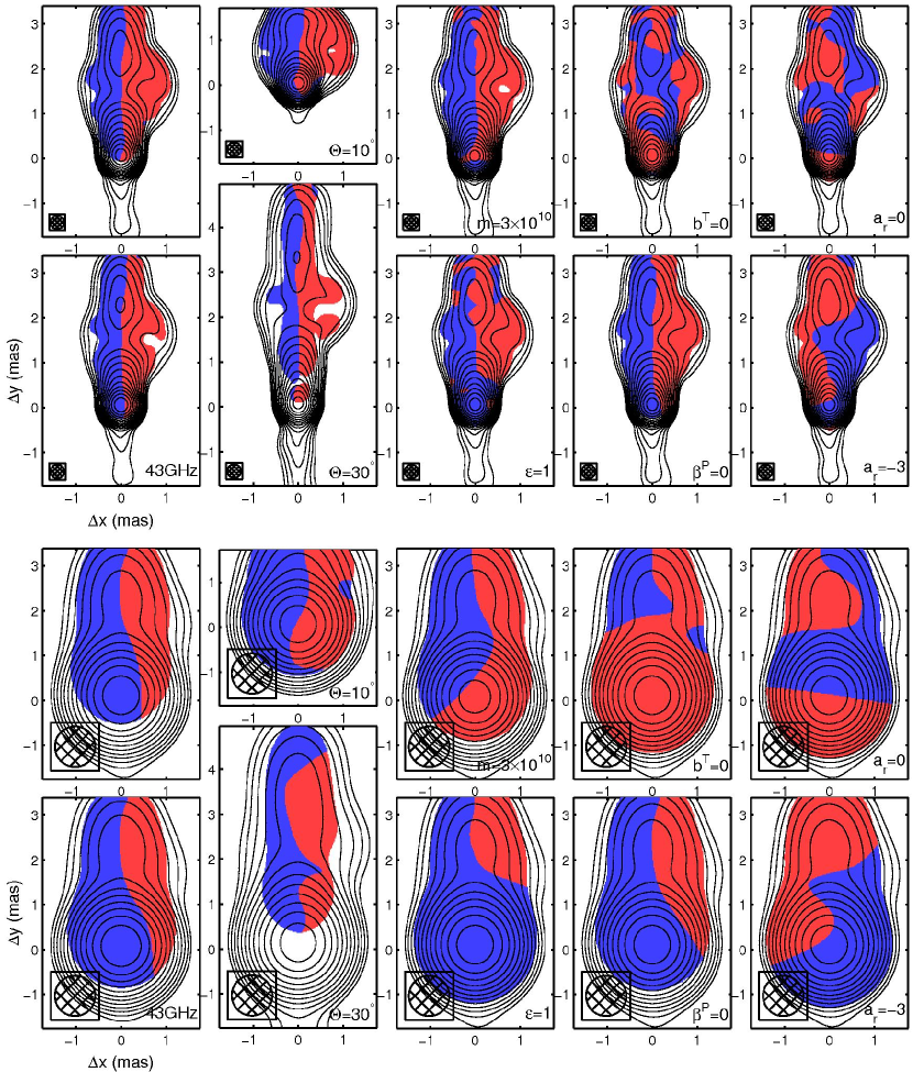
Figure 12: ${\rm sgn}({\rm RM})$ for an illustrative subset of the cases discussed in the text, compared to two examples of random foreground screens (rightmost maps). These are shown for two beam sizes, corresponding to resolved (top) and unresolved (bottom) jets. See the text and Table 3 for a complete list of relevant parameters for each, though the relevant defining parameter is listed as it appears in Figures 5–10 in the lower-right corner of each ${\rm sgn}({\rm RM})$ map. For reference total flux contours are overlayed, in logarithmic factors of 2, with the minimum contour corresponding to $0.98\,{\rm m}{\rm Jy}\,{\rm mas}^{-2}$. ${\rm RM}$s are shown only where the polarized flux exceeds $1{\rm m}{\rm Jy}\,{\rm mas}^{-2}$. In all maps the beam size is shown in the lower-left corner.

The proximity of the Faraday screen to the jet makes a strong prediction regarding the morphology of the ${\rm RM}$ maps. The presence of a large-scale radially correlated, toroidally dominated magnetic field within the jet sheath implies that the ${\rm RM}$ map will be strongly correlated along the jet. This has dramatic consequences for the ${\rm sgn}({\rm RM})$ maps, resulting in a very particular bilateral structure.

Example ${\rm sgn}({\rm RM})$ maps are presented for a variety of jet model and observational parameters in Figure 12. For two different beam widths, chosen to represent resolved and unresolved jets, ($0.3\,{\rm mas}$ and $0.9\,{\rm mas}$ on the top and bottom, respectively) we present the ${\rm sgn}({\rm RM})$ maps representative of the various parameters we have considered in Sections 3.1–3.3. Specifically, for each beam size we show the ${\rm sgn}({\rm RM})$ associated with our canonical model (upper left), at $43\,{\rm GHz}$ (lower left), high and low inclinations (upper and lower center-left, respectively), a black hole with $m=3\times 10^{10}$ (upper center), an efficiently heated Faraday screen (lower center), vanishing toroidal magnetic field (upper center-right) and vanishing poloidal velocity (lower center-right). The ${\rm sgn}({\rm RM})$ morphology is insensitive to the properties of the poloidal magnetic field and the toroidal velocity, though both can alter the details of the ${\rm sgn}({\rm RM})$ map.

With the exception of a vanishing toroidal magnetic field, all of the jet models listed above exhibit the afore mentioned bilateral morphology throughout the optically thin portion of the jet (as with the ${\rm RM}$ profiles, near the radio core departures from this structure can occur for some azimuthal orientations). This suggests that if the Faraday screen is close to the jet, the observation of such a structure in the ${\rm RM}$s of the optically thin portions of AGN jets is a robust indicator of the presence of ordered, toroidal magnetic fields. However, the strength of this evidence does depend upon the particulars of the jet model, and more importantly the beam resolution.

At small inclinations, insufficient radial range may exist to argue unambiguously for the correlated bilateral morphology. At large inclinations, the transverse structure of the jet may remain unresolved, leading to the previously-mentioned issues surrounding beam convolution. This is illustrated in the large-beam ${\rm sgn}({\rm RM})$ maps (Figure 12, bottom), in which the unresolved maps show relatively little structure in all cases. While it still appears possible to determine if ordered toroidal magnetic fields exist within the Faraday screen, the large beam limits the amount of asymmetric structure present when toroidal fields are sub-dominant. This difficulty vanishes when the transverse jet structure is resolved.

The morphology of the ${\rm sgn}({\rm RM})$ maps may also be used to observationally probe the location of the Faraday screen, ruling out contributions from distant, randomly oriented foreground clouds. While ${\rm pc}$-scale clouds have been detected via free-free absorption in a handful of sources (Jones et al., 1996; Walker et al., 2000), typically they are incapable of reproducing the large-scale radial correlations associated with Faraday rotation within the jet sheath. This may be argued on general grounds: Any model for the foreground Faraday screen must have structure on scales comparable to the jet width in order to mimic the observed transverse gradients. However, since in this case the Faraday screen is not associated with the jet itself, this implies that there must be structure parallel to the jet as well. Thus, we do not expect to see the bilateral morphology associated with the Faraday rotation due to a jet sheath.

To illustrate this explicitly, in the right-most panels of Figure 12 we show two examples of random distant foreground screens, in which $d{\rm RM}/d\ell$ is given by a Gaussian random field with power-law power spectra, $P_{k}\propto k^{a_{r}}$. To emphasize the diagnostic ability of the ${\rm sgn}({\rm RM})$ map, we subtract off the flux-weighted average ${\rm RM}$, which is degenerate with a Galactic contribution, in order to ensure that the ${\rm sgn}({\rm RM})$ map exhibits significant structure. These realizations are not intended to represent physical models for the plasma conditions within the Faraday screen. Rather, they simply provide two well-defined examples of the beam-convolved ${\rm sgn}({\rm RM})$ maps associated with foreground screens that are uncorrelated with the jet itself. In keeping with this motivation, we choose a flat spectrum ($a_{r}=0$), which necessarily produces considerable structure on angular scales comparable to the beam, and a red spectrum ($a_{r}=-3$) which typically generates structure on the largest relevant scale (e.g., the jet length).

The flat-spectrum foreground screen produces ${\rm sgn}({\rm RM})$ maps that are similar in structure to those arising when the toroidal magnetic field within the jet sheath vanishes. As a consequence, our discussion of the ${\rm sgn}({\rm RM})$ maps as indicators of the presence of ordered toroidal fields applies to the distinction between local and distant, flat-spectrum Faraday screens as well. That is, the presence of ordered, bilateral structures in the optically thin portions of the jet necessarily excludes this kind of distant screen.

The red-spectrum foreground screen is more problematic. In this case large-scale structures characteristic of red spectra are apparent, frequently extending substantial distances along the jet axis. As a result, distinguishing between red-spectra foregrounds and nearby Faraday rotation is difficult at large beam widths. This situation is ameliorated somewhat by smaller beams, at which not only the general morphology but also the detailed structure of the ${\rm sgn}({\rm RM})$ maps are apparent (cf. the canonical and red-spectrum models at small beams in Figure 12). Despite this, if the jet sheath is efficiently heated, this complication may remain, making the distinction between foreground and nearby Faraday rotation for any individual source challenging.

3.5 Implications for Jet Models

Because the ${\rm RM}$ depends upon the thermal particles that are directly modeled in jet theory, it provides a more robust handle upon the parameters of jet models. Thus, in addition to addressing prior suggestions about the source of the ${\rm RM}$s associated with AGN jets, we may also confront the observational applicability of our present understanding of how relativistic jets are produced and propagate.

First among these is the relationship between the nonthermal particles and the other jet parameters. By normalizing the accretion rate via the typical ${\rm RM}$ observed ($\sim 10^{3}\,{\rm rad}\,{\rm m}^{-2}$), we have been able to determine the efficiency with which the electromagnetic energy within the jet is dissipated into nonthermal particles producing the emission. For our canonical model we find that $\eta=0.02$ reproduces typical observed fluxes, meaning that the nonthermal particles constitute approximately $2\%$ of the energy density within the jet. This is roughly an order of magnitude larger than internal energy of the thermal particles within the jet. Therefore, when combined with ${\rm RM}$ measurements, their luminosity implies that at ${\rm pc}$-scales AGN jets are Poynting-dominated outflows of nonthermal, relativistic particles. This is consistent with some studies of ${\rm k}{\rm pc}$-scale AGN jets, finding that even at those scales large-scale fields persist and dominate the plasma thermal energy (see, e.g., Lapenta & Kronberg, 2005b).

Second, constraining the plasma parameters of the Faraday screen via ${\rm RM}$ profiles is complicated and will generally require careful modeling of the screen properties, e.g., via simulations like that we have presented here. This is because there are significant degeneracies between a number of otherwise poorly constrained properties; namely the jet orientation, bulk velocity of the rotating medium, thermal plasma density and temperature and the strength of the magnetic field. As seen in Figure 11, many of these are varying substantially throughout the screen. Furthermore, simplifying assumptions, such as equipartition, can be wrong by orders of magnitude. While it may be tempting to calibrate simple, qualitative models using simulations like the one we present, the relationship between the circum-jet material and the fast jet core is a strong function of black hole spin and other model parameters. Thus, efforts to quantitatively infer the properties of the circum-jet material will require additional, self-consistent jet formation simulations.

Third, we nevertheless find that the ordered toroidal magnetic field in the jet and its sheath were crucial to producing emission and Faraday rotation distributions that comport with observations. This is consistent with simplified, analytical efforts to explain these properties with a strongly-magnetized jet containing large-scale ordered toroidally dominated magnetic fields (see, e.g. Lyutikov et al., 2005). If AGN jets correspond well to GRMHD jet models like that presented here, observations of the ${\rm RM}$ gradients coupled with constraints upon the jet orientation, particle acceleration and heating rates within the jet and $\dot{M}$ as estimated by the disk thermal spectra and luminosity provide a means to estimate the jet power per unit mass accretion rate. For jets powered via the Blandford-Znajek mechanism, this quantity is a strong function of the black hole spin (McKinney, 2005; Tchekhovskoy et al., 2010), and hence may provide a means to measure the black hole spin magnitude for a large number of AGNs.

Fourth, it has been suggested that variations in the polarization angle across the jet indicate changes in the direction of the intrinsic magnetic field. Specifically, in a number of sources (e.g., 3C 272 and 1055+018) the polarization is aligned with the jet near the axis and becomes orthogonal to the jet at the edges (Attridge et al., 1999; Pushkarev et al., 2005; Zavala & Taylor, 2005; Gómez et al., 2008). Often this is considered evidence for a toroidally dominated jet core and a poloidally dominated jet sheath. However, studies of purely toroidal jets have qualitatively reproduced these polarization distributions as a consequence of projection effects and relativistic aberration (Lyutikov et al., 2005; Zakamska et al., 2008). Seen explicitly in Figure 3, our work also qualitatively reproduces the observed polarization structure without the need to appeal to variations in the intrinsic magnetic field geometry.

Finally, while the jet simulation is fully 3D, and this non-axisymmetric structure is clearly evident in the jet flux distributions, the resulting ${\rm RM}$ profiles are remarkably uniform (where they are sufficiently resolved). Thus, despite substantial departures from axisymmetry observed in the jet core, the assumption of axisymmetry in the surrounding medium seems well-justified.

4 Conclusions

It has now become possible to quantitatively compare ${\rm pc}$-scale observations of AGN jets with self-consistent fully 3D numerical GRMHD simulations of jets. Due to the need to model the nonthermal particles, direct comparisons between the emission and polarization properties of simulated and real jets are not possible, generally requiring additional post hoc assumptions about the poorly understood process of particle acceleration within the jet. In contrast, the ${\rm RM}$s associated with the circum-jet outflows depend only upon the simulated quantities. For these reasons AGN jet ${\rm RM}$s provide a potentially more robust diagnostic of the simulation parameters.

Even with relatively low accretion rates, $\sim 10^{-2}\dot{M}_{\rm Edd}$, we are able to reproduce the typical ${\rm RM}$s of $10^{3}\,{\rm rad}\,{\rm m}^{-2}$ observed in ${\rm pc}$-scale jets. These are generally proportional to $\dot{M}^{3/2}$, and thus even moderate increases in the accretion rate results in substantial increases in the typical ${\rm RM}$s. As a consequence it is possible to produce the majority of the observed Faraday rotation via propagation through the circum-jet material alone. Were the bulk of the observed ${\rm RM}$s to be produced far from the jet, this would require either $\dot{M}$s well below that necessary to produce the observed emission or very efficient dissipation of the magnetic field immediately outside of the jet (and thus very hot circum-jet plasma).

While well-separated from the emission region, the bulk of the Faraday rotation occurs in the immediate vicinity of the jet, within the surrounding jet sheath. This consists of a highly magnetized, relativistic outflow, which though moving more slowly than the jet core is more properly thought of as a continuous extension of the jet itself than a separate portion of the outflow. As a consequence, like the jet core, the magnetic field in the Faraday rotating jet sheath is dominated by a large-scale, ordered toroidal magnetic field.

The ${\rm RM}$ maps associated with our canonical model exhibit well-defined transverse ${\rm RM}$ gradients, associated primarily with the ordered toroidal magnetic field. Thus, our results suggest that efforts to probe the properties of toroidal magnetic fields in the circum-jet regions are consistent with existing 3D jet formation simulations, which self-consistently model the fast jet core and the surrounding Faraday rotating material. Furthermore, while some variation in the precise gradients across the jet exist due to non-axisymmetric jet structures, these are generally small in comparison to the gradients themselves, implying that ${\rm RM}$ observations can produce well-defined estimations of the toroidal field strength and structure.

The ${\rm RM}$ map details are also sensitive to the poloidal velocities, though in a way that is roughly degenerate with the dependence upon the mass accretion rate. However, at ${\rm pc}$ distances the comoving poloidal magnetic fields and toroidal velocities are sufficiently small that neither produce perturbations in the transverse ${\rm RM}$ profiles that exceed the variations associated with the non-axisymmetric structure of the jet. While this is dependent upon black hole mass, for reasonable values this implies that efforts to probe the poloidal magnetic field and toroidal velocities may be challenging.

Accurately measuring the ${\rm RM}$s of AGN jets depends critically upon the ability to resolve the jet’s transverse structure. This is generally violated in the radio core, and thus core ${\rm RM}$s and ${\rm RM}$-gradients may be typically unreliable. When the beam is moderately larger than the jet width finite beam effects result in a suppression of the ${\rm RM}$ relative to the true values, though well-defined gradients may still exist. When the beam is much larger, or when there is significant spectral or polarization structure on sub-beam scales, the resulting ${\rm RM}$s can be dramatically different from the true values. This motivates pushing towards higher frequencies and higher resolutions, as well as focusing upon resolved regions more than a beamwidth away from the radio core. For these purposes, space-based VLBI experiments like VSOP-2 are likely to be particularly useful.

The large-scale correlations along the jet indicative of ordered toroidal fields are present even in the ${\rm sgn}({\rm RM})$ maps, producing a distinctive, bilateral morphology. Models which invoke Faraday rotation far from the jet generally have difficulty reproducing this structure, and may therefore be excluded by ${\rm sgn}({\rm RM})$ measurements. Despite the fact that sufficiently red fluctuations in the foreground ${\rm RM}$s can mimic the long-range order indicative of toroidal fields, sufficiently resolved ${\rm RM}$ observations may robustly verify the presence of Faraday rotation in the vicinity of the jet.

While we have made an attempt to explore the various parameters critical to computing the ${\rm RM}$s of simulated jets, by no means has our investigation been exhaustive. The most significant limitation is the restriction to a single time step of a single jet simulation with a single prescription for the nonthermal particles. As a consequence we are not able to address the uncertainties in the ${\rm RM}$s associated with the substantial variability in the accretion onto the black hole. More importantly, we cannot address how interactions with the surrounding medium, known to be important in many cases, will affect our results. Where these interactions significantly alter the properties of the jet they should also make substantial changes to the particulars of the ${\rm RM}$ maps. However, since the general structure of the ${\rm RM}$s arise from a direct relationship with the order inherent in the jet’s magnetic field, we would expect the generic morphology of the ${\rm RM}$s to persist as long as the jet is toroidally dominated.

We thank Denise Gabuzda, Larwence Rudnick, Gregory Taylor and Philipp Kronberg for helpful comments and suggestions. This work was supported in part by NASA Chandra Fellowship PF7-80048 (JCM).

Appendix A Relativistic Aberration

In Section 2.3.2 we described how we performed the polarized radiative transfer through relativistically moving bulk flows. Here we present how the polarization direction changes due to relativistic aberration, and thus specifying the orientation of the parallely propagated orthonormal tetrad used to define the Stokes parameters. We will make use of four-vectors and covariant analysis, though the result will be quoted in terms of the three vectors we have used to define the relevant plasma quantities.

We choose to orient the Stokes parameters so that the projected, positive $z$-axis is “up” in the image plane. This is necessarily orthogonal to the wave four-vector, $k^{a}=(1,\mbox{\boldmath$\rm\hat{k}$})$, and thus,

$$e^{a}=(0,\mbox{\boldmath$\rm e$})-Ck^{a}\,,\quad\mbox{\boldmath$\rm e$}\equiv\mbox{\boldmath$\rm\hat{z}$}-\left(\mbox{\boldmath$\rm\hat{z}$}\cdot\mbox{\boldmath$\rm\hat{k}$}\right)\mbox{\boldmath$\rm\hat{k}$}\,,$$ (29)

in which $C$ is an arbitrary scalar. Generally, $e^{a}$ is only defined up to $C$, corresponding to the ambiguity associated with the time-component of the polarization four-vector in any given frame. Thus we are free to require $e^{a}$ be purely space-like in the jet frame, i.e., with $u^{a}=(\Gamma,\Gamma\mbox{\boldmath$\rm\beta$})$, we set $C$ such that $u^{a}e_{a}=0$, obtaining,

$$C=\frac{\mbox{\boldmath$\rm\beta$}\cdot\mbox{\boldmath$\rm e$}}{1-\mbox{\boldmath$\rm\beta$}\cdot\mbox{\boldmath$\rm\hat{k}$}}$$ (30)

This now defines the “up” direction, as seen in the jet frame.

In the emitter’s frame, the natural orientation for the Stokes parameters is aligned with the projected magnetic field, which is given by $\mbox{\boldmath$\rm b$}^{\prime}-(\mbox{\boldmath$\rm b$}^{\prime}\cdot\mbox{\boldmath$\rm\hat{k}$}^{\prime})\mbox{\boldmath$\rm\hat{k}$}^{\prime}$, where all primed quantities are in the jet frame (though note that $\hat{k}^{\prime}$ is the spatial components of $k^{a}$ in the jet frame, and thus is not unit-normalized). Thus,

$$\cos\xi =\frac{\hfil\mbox{\boldmath$\rm e$}^{\prime}\cdot\left[\mbox{\boldmath$\rm b$}^{\prime}-(\mbox{\boldmath$\rm b$}^{\prime}\cdot\mbox{\boldmath$\rm\hat{k}$}^{\prime})\mbox{\boldmath$\rm\hat{k}$}^{\prime}\right]}{|\mbox{\boldmath$\rm e$}^{\prime}||\mbox{\boldmath$\rm b$}^{\prime}-(\mbox{\boldmath$\rm b$}^{\prime}\cdot\mbox{\boldmath$\rm\hat{k}$}^{\prime})\mbox{\boldmath$\rm\hat{k}$}^{\prime}|}$$ (31)

$$=\frac{\hfil\mbox{\boldmath$\rm e$}^{\prime}\cdot\mbox{\boldmath$\rm b$}^{\prime}}{\sqrt{e^{a}e_{a}\left[b^{2}-(b^{a}k_{a}/u^{a}k_{a})^{2}\right]}}$$

$$=\frac{e^{a}b_{a}}{\sqrt{e^{a}e_{a}\left[b^{2}-(b^{a}k_{a}/u^{a}k_{a})^{2}\right]}}\,,$$

where we repeatedly used the fact that $e^{a}$ and $b^{a}$ are purely space-like in the jet frame. Via explicit computation, we have in the lab frame

$$e^{a}e_{a} =\hfil\hfil\mbox{\boldmath$\rm e$}\cdot\mbox{\boldmath$\rm e$}=1-\left(\hfil\mbox{\boldmath$\rm\hat{z}$}\cdot\mbox{\boldmath$\rm\hat{k}$}\right)^{2}$$ (32)

$$e^{a}b_{a} =\hfil\hfil\mbox{\boldmath$\rm e$}\cdot\mbox{\boldmath$\rm b$}-\frac{\Gamma\hfil\mbox{\boldmath$\rm\beta$}\cdot\mbox{\boldmath$\rm e$}}{u^{a}k_{a}}k^{b}b_{b}$$

$$=\hfil\hfil\mbox{\boldmath$\rm e$}\cdot\mbox{\boldmath$\rm b$}+\Gamma\hfil\hfil\mbox{\boldmath$\rm\beta$}\cdot\mbox{\boldmath$\rm e$}b\cos\vartheta$$

$$\frac{b^{a}k_{a}}{u^{b}k_{b}} =-b\cos\vartheta\,.$$

Therefore,

$$\cos\xi=\frac{\mbox{\boldmath$\rm e$}\cdot\left(\mbox{\boldmath$\rm b$}+\Gamma\mbox{\boldmath$\rm\beta$}b\cos\vartheta\right)}{\sqrt{1-\left(\mbox{\boldmath$\rm\hat{z}$}\cdot\mbox{\boldmath$\rm\hat{k}$}\right)^{2}}b\sin\vartheta}\,,$$ (33)

which reduces to Equation (12) upon noting that $\mbox{\boldmath$\rm e$}=\left(\mbox{\boldmath$\rm 1$}-\mbox{\boldmath$\rm\hat{k}$}\mbox{\boldmath$\rm\hat{k}$}\right)\cdot\mbox{\boldmath$\rm\hat{z}$}$

References

- Asada et al. (2008a) Asada, K., Inoue, M., Kameno, S., & Nagai, H. 2008a, ApJ, 675, 79
- Asada et al. (2008b) Asada, K., Inoue, M., Nakamura, M., Kameno, S., & Nagai, H. 2008b, ApJ, 682, 798
- Asada et al. (2008c) —. 2008c, ApJ, 682, 798
- Asada et al. (2004) Asada, K., Inoue, M., Uchida, Y., & Kameno, S. 2004, in Coevolution of Black Holes and Galaxies, ed. L. C. Ho
- Asada et al. (2002) Asada, K., Inoue, M., Uchida, Y., Kameno, S., Fujisawa, K., Iguchi, S., & Mutoh, M. 2002, PASJ, 54, L39
- Attridge et al. (1999) Attridge, J. M., Roberts, D. H., & Wardle, J. F. C. 1999, ApJ, 518, L87
- Beckwith & Done (2005) Beckwith, K., & Done, C. 2005, MNRAS, 359, 1217
- Beckwith et al. (2008) Beckwith, K., Hawley, J. F., & Krolik, J. H. 2008, ApJ, 678, 1180
- Blandford (1993) Blandford, R. 1993, in Astrophysics and Space Science Library, Vol. 103, Astrophysics and Space Science Library, 15–33
- Blandford & Znajek (1977) Blandford, R. D., & Znajek, R. L. 1977, MNRAS, 179, 433
- Broderick & Blandford (2004) Broderick, A., & Blandford, R. 2004, MNRAS, 349, 994
- Broderick (2006) Broderick, A. E. 2006, MNRAS, 366, L10
- Broderick & Loeb (2006) Broderick, A. E., & Loeb, A. 2006, MNRAS, 367, 905
- Broderick & Loeb (2009) —. 2009, ApJ, 703, L104
- Bromley et al. (2001) Bromley, B. C., Melia, F., & Liu, S. 2001, ApJ, 555, L83
- Burbidge (1956) Burbidge, G. R. 1956, ApJ, 124, 416
- Burn (1966) Burn, B. J. 1966, MNRAS, 133, 67
- Connors & Stark (1977) Connors, P. A., & Stark, R. F. 1977, Nature, 269, 128
- Connors et al. (1980) Connors, P. A., Stark, R. F., & Piran, T. 1980, ApJ, 235, 224
- Cotton et al. (2003) Cotton, W. D., Dallacasa, D., Fanti, C., Fanti, R., Foley, A. R., Schilizzi, R. T., & Spencer, R. E. 2003, A&A, 406, 43
- Croke et al. (2010) Croke, S. M., O’Sullivan, S. P., & Gabuzda, D. C. 2010, MNRAS, 402, 259
- Gabuzda & Chernetskii (2003) Gabuzda, D. C., & Chernetskii, V. A. 2003, MNRAS, 339, 669
- Gabuzda et al. (2004) Gabuzda, D. C., Murray, É., & Cronin, P. 2004, MNRAS, 351, L89
- Gabuzda et al. (2000) Gabuzda, D. C., Pushkarev, A. B., & Cawthorne, T. V. 2000, MNRAS, 319, 1109
- Gammie et al. (2003) Gammie, C. F., McKinney, J. C., & Tóth, G. 2003, ApJ, 589, 444
- Gardner & Whiteoak (1966) Gardner, F. F., & Whiteoak, J. B. 1966, ARA&A, 4, 245
- Gómez et al. (2008) Gómez, J. L., Marscher, A. P., Jorstad, S. G., Agudo, I., & Roca-Sogorb, M. 2008, ApJ, 681, L69
- Gracia et al. (2009) Gracia, J., Vlahakis, N., Agudo, I., Tsinganos, K., & Bogovalov, S. V. 2009, ApJ, 695, 503
- Hawley & Krolik (2006) Hawley, J. F., & Krolik, J. H. 2006, ApJ, 641, 103
- Huang et al. (2008) Huang, L., Liu, S., Shen, Z., Cai, M. J., Li, H., & Fryer, C. L. 2008, ApJ, 676, L119
- Jaroszynski & Kurpiewski (1997) Jaroszynski, M., & Kurpiewski, A. 1997, A&A, 326, 419
- Jones et al. (1996) Jones, D. L., et al. 1996, ApJ, 466, L63+
- Jorstad et al. (2005) Jorstad, S. G., et al. 2005, AJ, 130, 1418
- Kharb et al. (2009) Kharb, P., Gabuzda, D. C., O’Dea, C. P., Shastri, P., & Baum, S. A. 2009, ApJ, 694, 1485
- Kigure et al. (2004) Kigure, H., Uchida, Y., Nakamura, M., Hirose, S., & Cameron, R. 2004, ApJ, 608, 119
- Koenigl & Choudhuri (1985) Koenigl, A., & Choudhuri, A. R. 1985, ApJ, 289, 173
- Komissarov et al. (2007) Komissarov, S. S., Barkov, M. V., Vlahakis, N., & Königl, A. 2007, MNRAS, 380, 51
- Laing & Bridle (2002a) Laing, R. A., & Bridle, A. H. 2002a, MNRAS, 336, 1161
- Laing & Bridle (2002b) —. 2002b, MNRAS, 336, 328
- Laing et al. (2006a) Laing, R. A., Canvin, J. R., & Bridle, A. H. 2006a, Astronomische Nachrichten, 327, 523
- Laing et al. (2006b) Laing, R. A., Canvin, J. R., Cotton, W. D., Bridle, A. H., & Parma, P. 2006b, Astronomische Nachrichten, 327, 533
- Laor et al. (1990) Laor, A., Netzer, H., & Piran, T. 1990, MNRAS, 242, 560
- Lapenta & Kronberg (2005a) Lapenta, G., & Kronberg, P. P. 2005a, ApJ, 625, 37
- Lapenta & Kronberg (2005b) —. 2005b, ApJ, 625, 37
- Lindquist (1966) Lindquist, R. W. 1966, Anals of Physics, 37, 487
- Lister et al. (1998) Lister, M. L., Marscher, A. P., & Gear, W. K. 1998, ApJ, 504, 702
- Lovelace et al. (2002) Lovelace, R. V. E., Li, H., Koldoba, A. V., Ustyugova, G. V., & Romanova, M. M. 2002, ApJ, 572, 445
- Lynden-Bell (1996) Lynden-Bell, D. 1996, MNRAS, 279, 389
- Lyubarsky (2005) Lyubarsky, Y. E. 2005, MNRAS, 358, 113
- Lyutikov (2006) Lyutikov, M. 2006, New Journal of Physics, 8, 119
- Lyutikov et al. (2005) Lyutikov, M., Pariev, V. I., & Gabuzda, D. C. 2005, MNRAS, 360, 869
- Lyutikov & Uzdensky (2003) Lyutikov, M., & Uzdensky, D. 2003, ApJ, 589, 893
- Mahmud et al. (2009) Mahmud, M., Gabuzda, D. C., & Bezrukovs, V. 2009, MNRAS, 400, 2
- McKinney (2005) McKinney, J. C. 2005, ApJ, 630, L5
- McKinney (2006) —. 2006, MNRAS, 368, 1561
- McKinney & Blandford (2009) McKinney, J. C., & Blandford, R. D. 2009, MNRAS, 394, L126
- McKinney & Gammie (2004) McKinney, J. C., & Gammie, C. F. 2004, ApJ, 611, 977
- Nakamura et al. (2008) Nakamura, M., Tregillis, I. L., Li, H., & Li, S. 2008, ApJ, 686, 843
- Nakamura et al. (2001) Nakamura, M., Uchida, Y., & Hirose, S. 2001, New Astronomy, 6, 61
- O’Sullivan & Gabuzda (2009a) O’Sullivan, S. P., & Gabuzda, D. C. 2009a, MNRAS, 400, 26
- O’Sullivan & Gabuzda (2009b) —. 2009b, MNRAS, 393, 429
- Pushkarev et al. (2005) Pushkarev, A. B., Gabuzda, D. C., Vetukhnovskaya, Y. N., & Yakimov, V. E. 2005, MNRAS, 356, 859
- Reynolds et al. (2001) Reynolds, C., Cawthorne, T. V., & Gabuzda, D. C. 2001, MNRAS, 327, 1071
- Sharma et al. (2007) Sharma, P., Quataert, E., & Stone, J. M. 2007, ApJ, 671, 1696
- Shcherbakov (2008) Shcherbakov, R. V. 2008, ApJ, 688, 695
- Sikora et al. (2005) Sikora, M., Begelman, M. C., Madejski, G. M., & Lasota, J. 2005, ApJ, 625, 72
- Tchekhovskoy et al. (2009a) Tchekhovskoy, A., McKinney, J. C., & Narayan, R. 2009a, ApJ, 699, 1789
- Tchekhovskoy et al. (2009b) Tchekhovskoy, A., Narayan, R., & McKinney, J. C. 2009b, astro-ph/0909.0011
- Tchekhovskoy et al. (2010) —. 2010, ApJ, 711, 50
- Tsuboi et al. (2009) Tsuboi, M., et al. 2009, in Astronomical Society of the Pacific Conference Series, Vol. 402, Astronomical Society of the Pacific Conference Series, ed. Y. Hagiwara, E. Fomalont, M. Tsuboi, & M. Yasuhiro, 30
- Uchida et al. (2004) Uchida, Y., Kigure, H., Hirose, S., Nakamura, M., & Cameron, R. 2004, ApJ, 600, 88
- Udomprasert et al. (1997) Udomprasert, P. S., Taylor, G. B., Pearson, T. J., & Roberts, D. H. 1997, ApJ, 483, L9+
- Vlahakis & Königl (2004) Vlahakis, N., & Königl, A. 2004, ApJ, 605, 656
- Walker et al. (2000) Walker, R. C., et al. 2000, ApJ, 530, 233
- Zakamska et al. (2008) Zakamska, N. L., Begelman, M. C., & Blandford, R. D. 2008, ApJ, 679, 990
- Zavala & Taylor (2001) Zavala, R. T., & Taylor, G. B. 2001, ApJ, 550, L147
- Zavala & Taylor (2002) —. 2002, ApJ, 566, L9
- Zavala & Taylor (2003) —. 2003, ApJ, 589, 126
- Zavala & Taylor (2004) —. 2004, ApJ, 612, 749
- Zavala & Taylor (2005) —. 2005, ApJ, 626, L73
- Zhang & Nan (2001) Zhang, H. Y., & Nan, R. D. 2001, Ap&SS, 278, 143