Excitation of the molecular gas in the nuclear region of M 82

We present high-resolution HIFI spectroscopy of the nucleus of the archetypical starburst galaxy M 82. Six $\@element[12]{\mathrm{C}}$O lines, 2 $\@element[13]{\mathrm{C}}$O lines and 4 fine-structure lines have been detected. Besides showing the effects of the overall velocity structure of the nuclear region, the line profiles also indicate the presence of multiple components with different optical depths, temperatures, and densities in the observing beam. The data have been interpreted using a grid of PDR models. It is found that the majority of the molecular gas is in low density ($n=10^{3.5}$ cm^-3) clouds, with column densities of $N_{\rm H}=10^{21.5}$ cm^-2 and a relatively low UV radiation field ($G_{0}$= $10^{2}$). The remaining gas is predominantly found in clouds with higher densities ($n=10^{5}$ cm^-3) and radiation fields ($G_{0}$= $10^{2.75}$), but somewhat lower column densities ($N_{\rm H}=10^{21.2}$ cm^-2). The highest $J$ CO lines are dominated by a small (1% relative surface filling) component, with an even higher density ($n=10^{6}$ cm^-3) and UV field ($G_{0}$= $10^{3.25}$). These results show the strength of multi-component modelling for interpretating the integrated properties of galaxies.

1 Introduction

M 82 is one of the best studied starburst galaxies in the local universe. Its short distance (3.9 Mpc, Sakai & Madore 1999) makes it a superb candidate for detailed studies of the physical processes related to star formation and their effects on the galaxy. The emission from the interstellar medium (ISM) is an excellent tool for diagnosing the physical and chemical properties of the star-forming environment. Over the past decades, M 82 has been studied in many atomic and molecular species. These observations show a complex environment where multiple components with different excitation, temperatures, densities, and filling factors coexists (e.g., Wild et al. 1992; Lord et al. 1996; Mao et al. 2000; Weiß et al. 2001; Ward et al. 2003; Spaans & Meijerink 2007; Fuente et al. 2008).

In this paper we present observations of the nucleus of M 82 using the Heterodyne Instrument for the Far Infrared (HIFI, De Graauw et al., 2010) on board of the ESA Herschel Space Observatory as part of the HEXGAL key programme (PI R. Güsten). Due to the large spectral coverage available with Herschel, we can observe a large number of lines, enabling comprehensive study of the excitation of the different ISM components. At the same time, the high spectral resolution provided by HIFI makes it possible to separate different velocity components. In this paper, we combine these observations with detailed modelling to derive the physical conditions and excitation mechanisms of the nuclear ISM of M 82.

2 Observations, reduction, and results

The observations were performed in two blocks during April 17-19 and May 03, 2010. Selected CO transitions and their $\@element[13]{\mathrm{C}}$O isotopomers, as well as fine-structure lines of [C I], [C II], and [N II], were observed (see Table 1 and Fig. 1) in the nuclear region of M 82 (RA 09h55m52.22s, Dec 69d40m46.9s J2000). The observations were carried out in dual-beam switch mode with standard 3′ beam-chopping in the “fast” mode with chop rates between 0.2 and 2 Hz to improve stability. Relevant details of the observations are summarized in Table 1.

2.1 Data reduction

Initial data processing was done using HIPE version 2.9. A modified version of the level 2 pipeline was used that does not time average the data, in order to inspect the individual subscans in observations that contain more than one subscan. After inspection, the subscans were averaged and the subbands were stitched together.

Further analysis of the data was done using the CLASS package. The data were binned until a sufficiently high signal to noise ratio was achieved. Linear baselines were subtracted, excluding parts of the baseline that contained lines or seemed affected by instabilities. After this subtraction, the $\@element[13]{\mathrm{C}}$O ($5-4$) and $\@element[13]{\mathrm{C}}$O ($6-5$) spectra showed residual baseline structure. Since these structures are not seen in the $\@element[12]{\mathrm{C}}$O ($5-4$) and $\@element[12]{\mathrm{C}}$O ($6-5$) spectra, they were assumed to be baseline instabilities and were removed by fitting a 4^th order polynomial.

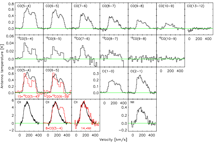
Figure 1: Observed spectra. Both polarizations were averaged in these spectra. Velocities are heliocentric.

2.2 Spectra

Figure 1 shows the resulting spectra, obtained by averaging both polarizations. Six CO lines, 2 $\@element[13]{\mathrm{C}}$O lines, and all 4 targeted fine-structure lines are detected. Three lines are clear non-detections: CO ($13-12$), $\@element[13]{\mathrm{C}}$O ($9-8$), and $\@element[13]{\mathrm{C}}$O ($10-9$). The $\@element[13]{\mathrm{C}}$O ($7-6$) line can be seen in the spectrum, but the integrated flux can not be securely determined due to severe baseline instabilities. The $\@element[13]{\mathrm{C}}$O ($8-7$) observations also suffer from baseline problems between $\sim$ 400 and 700 km s^-1, making it impossible to determine a good baseline and establish the presence of a line. Because of the high frequency of the lines, the [C II] and [N II] spectra cover only a narrow range, and therefore a baseline can only be fit to the outer channels.

2.3 Line fluxes

The CO emission in M 82 has two main velocity components (the southwest (SW, v${}_{\rm hel}\sim$160 km s^-1) and northeast (NE, v${}_{\rm hel}\sim$300 km s^-1) lobes; see e.g., Fig. 2 and Wild et al. 1992), which can also be seen in our data. Therefore, two Gaussian profiles are fitted to each spectrum. The size of the beam varies for the different frequencies, ranging from 12″ for the [C II] observations to 44″ at the lowest frequency ([C I] 609 $\mu$m). To be able to compare the observations to each other and to the model results, all observations are scaled to the largest beam. The scaling factor ($\kappa_{s}$) is calculated by convolving a 450 $\mu$m SCUBA map with a resolution of 7″ (taken from the SCUBA archive) with Gaussian profiles with the size of the different beams, to estimate the flux contained in those beams. The value of $\kappa_{s}$ is calculated by taking the ratio of the integrated 450 $\mu$m flux for each beam with the flux contained in the largest beam. This results in values for $\kappa_{s}$ between 1 and 0.19 (see Table 1). Since the calibration of HIFI is still preliminary, theoretical predictions (Kramer 2006) are used to convert the antenna temperatures into flux densities (see Table 1). After applying the beam corrections and the preliminary calibration, the final CO fluxes are very similar (within 10%) to the fluxes measured with SPIRE, which are corrected for source-beam coupling using a 250 $\mu$m SPIRE map (Panuzzo et al. 2010). The final corrected fluxes are listed in Table 1, together with the 1$\sigma$ uncertainties derived from the fits. Given the uncertainties in the pointing and calibration, we apply an additional error to the fluxes, when comparing them to the models. This error will increase with frequency; however, since the exact frequency dependence is unknown, an average value of 30% is used.

3 Analysis and discussion

The spectra in Fig. 1 show well-resolved line profiles, which provide important boundary conditions for further analysis. Most lines show the two main velocity components: the blue-shifted SW and the red-shifted NE emission lobes. The [N II] and [C II] lines show spectra that are dominated by the blue-shifted component. This can occur because the beam at these frequencies is so small (see beam size bars overlayed on Fig. 2) that the NE lobe is not covered. Our observing position is shown in Fig. 3 of Weiß et al. (this volume), where various beam sizes are also indicated, showing the extent to which the two lobes are covered at various frequencies.

Inspection of the $\@element[12]{\mathrm{C}}$O line profiles shows that at low $J$ the SW lobe, peaking at 160 km s^-1, dominates the blue-shifted emission component. Going to higher $J$, an additional feature peaking at 100 km s^-1 becomes increasingly important and is brighter than the 160 km s^-1 peak at $J>8$. This feature dominates the $\@element[13]{\mathrm{C}}$O lines already at $J=5-4$. $\@element[12]{\mathrm{C}}$O ($3-2$) and $\@element[12]{\mathrm{C}}$O ($6-5$) position-velocity diagrams (Fig. 2, data taken from the JCMT archive) show that this 100 km s^-1 feature corresponds to a separate structure in the SW lobe. The change in contribution of this feature for different transitions and isotopomers indicates that it has physical properties different from the neighbouring 160 km s^-1 feature. This demonstrates that M 82 contains star-forming regions with different physical properties, such as optical depth, temperature, and density, in the observing beam. This information only becomes available with the velocity-resolved line profiles provided by HIFI.

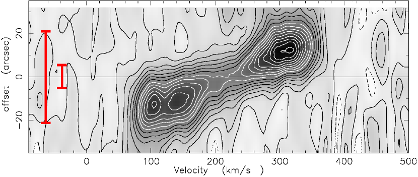
Figure 2: Position-velocity diagram of the Nucleus of M 82, observed in $\@element[12]{\mathrm{C}}$O($6-5$). Vertical resolution and beam size are $\sim$16″. The two red bars show the largest (44″) and (12″) smallest beams in our observations.

3.1 CO excitation

The NE and SW lobes, unlike the 100 km s^-1 spectral feature, do not show any difference in behaviour. They merely reflect the kinematics of M 82 and will both have contributions from different physical components of the ISM. Because of this and the 100 km s^-1 component being too weak in most lines to be fit separately, we analyse the CO excitation using the integrated line strengths, but explicitly allowing for the presence of multiple excitation components.

We combined our data with ground-based observations of CO ($1-0$) to CO ($4-3$), CO ($6-5$), CO ($7-6$), and $\@element[13]{\mathrm{C}}$O ($1-0$) to $\@element[13]{\mathrm{C}}$O ($3-2$) (Ward et al. 2003) and the SPIRE detections of CO ($4-3$) to CO ($13-12$), $\@element[13]{\mathrm{C}}$O ($5-4$), $\@element[13]{\mathrm{C}}$O ($7-6$), and $\@element[13]{\mathrm{C}}$O ($8-7$) (Panuzzo et al. 2010). Ward et al. (2003) present separate observations of the two lobes. Since both fit within our largest beam, we added the fluxes. The ground-based data have been scaled to match our observations, using the CO ($6-5$) and CO ($7-6$) lines. Both the Ward et al. (2003) and Panuzzo et al. (2010) data have already been corrected for source-beam coupling factors. This resulted in the two CO excitation diagrams shown in Fig. 3.

The CO and the fine-structure line ratios are compared to the results of a large grid of photon-dominated region (PDR) models (Meijerink & Spaans 2005; Meijerink et al. 2007). The $\@element[12]{\mathrm{C}}$O/$\@element[13]{\mathrm{C}}$O abundance ratio is fixed at a value of 40 (similar to the value found by Ward et al. 2003). The comparison with the CO lines is shown in Fig. 3. The observations can be best reproduced with a combination of one low and two high-density components. The low-density component, which dominates in the lowest CO lines ($J\leq 3$), is found to have a density of $n=10^{3.5}$ cm^-3 and a UV flux of $G_{0}$= $10^{2}$. This component represents the extended molecular ISM. The mid-$J$ CO lines ($4<J<7$) are mostly produced by clouds that have a density of $n=10^{5}$ cm^-3 and a radiation field of $G_{0}$= $10^{2.75}$. At transitions higher than 7 (and $\@element[13]{\mathrm{C}}$O $J>5$), the line emission comes from clouds with even higher densities ($n=10^{6}$ cm^-3) and radiation fields ($G_{0}$= $10^{3.25}$). These two models represent the dense, star-forming molecular clouds. The densest component has parameters similar to hot cores in the Milky Way. This component has excitation properties similar to the $100\,$km s^-1 feature detected in our spectra as can be seen by comparing the $\@element[12]{\mathrm{C}}$O and $\@element[13]{\mathrm{C}}$O ($6-5$) lines in the models.

Since we have $\@element[13]{\mathrm{C}}$O lines for both the low- ($J\leq 3$) and high-density ($J\geq 4$) components, it is possible to determine the column density for both. The low-density component is found to have a slightly higher column density ($N_{\rm H}=10^{21.5}$ cm^-2) than the high-density component ($N_{\rm H}=10^{21.2}$ cm^-2). This is reflected in the $\@element[12]{\mathrm{C}}$O/$\@element[13]{\mathrm{C}}$O line ratios, which increase from 14.5 for the $J=1-0$ to 27.2 for the $J=8-7$ transition.

The relative scaling of the three models provides an estimate of the relative beam filling of the components and was found to be 70%:29%:1% for the low density, high density low $G_{0}$, and high density high $G_{0}$ components, respectively.

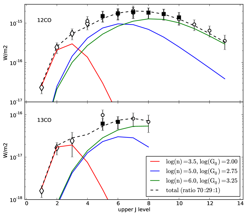
Figure 3: Excitation of $\@element[12]{\mathrm{C}}$O and $\@element[13]{\mathrm{C}}$O. Solid squares represent HIFI observations presented in this work, and open diamonds and circles data are taken from Ward et al. (2003) and Panuzzo et al. (2010), respectively. Lines represent the result of PDR models. See legend and text for more information on the models.

Table 1: Observation parameters and observed line fluxes, where fluxes include beam correction and calibration.

Line	Freq	$\lambda$	Band	tint	Beam	$\kappa_{s}$	$\eta_{MB}$	TA$\rightarrow$Jy	Blue	Red	Total
	[GHz]	[ $\mu$m]		[sec]	[″]			[Jy K-1]	[$10^{3}$ Jy km s-1]	[$10^{3}$ Jy km s-1]	[$10^{3}$ Jy km s-1]
CO $J=5-4$	576	520	1b	250	38	0.87	0.69	474	44.2$\pm$0.4	34.3$\pm$0.4	78.5$\pm$0.6
CO $J=6-5$	691	434	2a	248	33	0.77	0.68	481	44.2$\pm$0.8	32.5$\pm$0.8	76.6$\pm$1.2
CO $J=7-6$	807	372	3a	248	27	0.61	0.68	481	40.6$\pm$1.6	30.5$\pm$1.7	71.2$\pm$2.3
CO $J=8-7$	922	325	3b	250	25	0.55	0.68	481	33.8$\pm$2.6	26.4$\pm$2.7	60.2$\pm$3.8
CO $J=9-8$	1037	289	4a	306	23	0.48	0.67	488	31.4$\pm$1.4	18.0$\pm$1.4	49.3$\pm$2.0
CO $J=10-9$	1152	260	5a	334	20	0.40	0.67	488	16.9$\pm$3.7	19.5$\pm$4.3	36.4$\pm$5.7
$\@element[13]{\mathrm{C}}$O$J=5-4$	551	544	1a	314	44	1.00	0.69	474	2.0$\pm$0.1	1.3$\pm$0.1	3.4$\pm$0.2
$\@element[13]{\mathrm{C}}$O$J=6-5$	661	453	2a	306	33	0.77	0.68	481	2.3$\pm$0.3	0.8$\pm$0.2	3.1$\pm$0.4
[C I] ${}^{3}P_{1}-^{3}P_{0}$	492	609	1a	248	44	1.00	0.69	474	13.3$\pm$0.6	8.2$\pm$0.6	21.5$\pm$0.8
[C I] ${}^{3}P_{2}-^{3}P_{1}$	809	369	3a	306	27	0.61	0.68	481	22.2$\pm$1.9	20.3$\pm$2.1	42.5$\pm$2.8
[C II] ${}^{2}P_{3/2}-^{2}P_{1/2}$	1901	158	7b	306	12	0.19	0.63	519	1051.4$\pm$57.6	1262.7$\pm$57.0	2314.1$\pm$81.1
[N II] ${}^{3}P_{1}-^{3}P_{0}$	1461	205	6a	507	15	0.27	0.65	503	58.0$\pm$39.1	66.7$\pm$39.1	124.7$\pm$55.3

3.2 Fine-structure lines

To further constrain the modelling results, we also considered fine-structure line ratios. The ratio between the two [C I] lines is sensitive to the impinging UV flux (see Meijerink et al. 2007). Line ratios with [C II] and [N II] may provide additional insight into the ionization balance. Because of the different shapes of the red component of the [C II] and [N II] lines, we do not use the total integrated flux of those lines. Instead, the blue component is scaled using the average total/blue ratio.

The model prediction for the [C I] 609 $\mu$m/[C I] 369 $\mu$m line ratio (0.28) is close to the observed value (0.31). This is surprising since [C I] 609 $\mu$m is usually observed to be stronger than predicted by models or observed in the Milky Way (e.g., White et al. 1994; Israel & Baas 2002). That our prediction is close to the observed value stems from our multi-component modelling. The low-density component has a ratio that is higher than observed, and the high-density components have lower ratios, resulting in an average that is close to the observed value.

The models under-predict the [C II]/[C I] ratios by about a factor of three higher. This excess in [C II] emission likely arises from the diffuse, ionized ISM, which is confirmed by the similarity of the [C II] and [N II] line shapes of the blue lobe.

To address the uniqueness of our model, a model with only one high-density component was also attempted. The best fit is found using a lower density ($n=10^{4.25}$ cm^-3) and a high radiation field ($G_{0}$= $10^{3.5}$). Also a much higher surface ratio is needed (ratio of low- to high-density components 20%:80%). Although this model is able to fit the $\@element[12]{\mathrm{C}}$O excitation within the error bars, it underpredicts the strength of the $\@element[13]{\mathrm{C}}$O lines by factors of a few. Also the predicted [C II]/[C I] ratios are an order of magnitude too high and, therefore, a two component interpretation, such as done by Panuzzo et al. (2010), is insufficient for modelling the CO excitation in M82. This conclusion is reinforced by earlier analyses by e.g., based on large velocity gradient analysis of multiple CO lines (e.g., Wild et al. 1992; Güsten et al. 1993; Weiß et al. 2001; Ward et al. 2003; Weiß et al. 2005)

4 Summary and outlook

The CO and fine-structure lines provide an excellent tool for determining the physical parameters of the nuclear ISM of M 82. The line shapes reveal distinct velocity components at 100, 160, and 300 km s^-1. While the 160 and 300 km s^-1 features reflect the large-scale kinematics of M 82, the 100 km s^-1 feature shows an excitation different from the other components, which is only revealed by the velocity-resolved HIFI data. The presence of multiple ISM components with different physical conditions is also found in modelling of the CO lines, which shows that three density components are needed to explain the observed line fluxes.

The majority of the gas is in low density ($n=10^{3.5}$ cm^-3) clouds, with column densities of $N_{\rm H}=10^{21.5}$ cm^-2 and a relatively low UV radiation field ($G_{0}$= $10^{2}$). The remaining gas is predominantly found in clouds with higher densities ($n=10^{5}$ cm^-3) and radiation fields ($G_{0}$= $10^{2.75}$), but lower column densities ($N_{\rm H}=10^{21.2}$ cm^-2). The highest $J$ CO lines are dominated by a small (1% relative surface filling) component, with an even higher density ($n=10^{6}$ cm^-3) and UV field ($G_{0}$= $10^{3.25}$).

Using the unique spectral coverage and resolution offered by HIFI, we are one step closer to correctly dissecting the intricate and interacting density components and excitation regimes present in the core of M 82. Additional observations (part of the HEXGAL programme) of the lobes of M 82 and of other starburst galaxies will increase our understanding of such systems even more.