Probing Hot Gas in Galaxy Groups through the Sunyaev-Zeldovich Effect

Abstract

We investigate the potential of exploiting the Sunyaev-Zeldovich effect (SZE) to study the properties of hot gas in galaxy groups. It is shown that, with upcoming SZE surveys, one can stack SZE maps around galaxy groups of similar halo masses selected from large galaxy redshift surveys to study the hot gas in halos represented by galaxy groups. We use various models for the hot halo gas to study how the expected SZE signals are affected by gas fraction, equation of state, halo concentration, and cosmology. Comparing the model predictions with the sensitivities expected from the SPT, ACT and Planck surveys shows that a SPT-like survey can provide stringent constraints on the hot gas properties for halos with masses $M\lower 3.01385pt\hbox{$\;\buildrel>\over{\sim}\;$}10^{13}\>h^{-1}\rm M_{\odot}$. We also explore the idea of using the cross correlation between hot gas and galaxies of different luminosity to probe the hot gas in dark matter halos without identifying galaxy groups to represent dark halos. Our results show that, with a galaxy survey as large as the Sloan Digital Sky Survey and with the help of the conditional luminosity function (CLF) model, one can obtain stringent constraints on the hot gas properties in halos with masses down to $10^{13}\>h^{-1}\rm M_{\odot}$. Thus, the upcoming SZE surveys should provide a very promising avenue to probe the hot gas in relatively low-mass halos where the majority of $L^{*}$-galaxies reside.

1 introduction

In the current cold dark matter (CDM) paradigm, the large-scale structure in the Universe grows due to gravitational instability, forming dark matter halos within which galaxies form. Since the cosmic gas is initially cold and well mixed with the dark matter, the gas component is expected to follow the evolution of the dark matter component until it is heated by accretion shocks during halo formation, resulting in extended gaseous halos that trace out the potential wells of dark matter halos. In the simplest case where the process is assumed to be non-radiative, the total amount of hot gas contained in a gaseous halo is expected to be roughly the amount of gas initially associated with the dark matter halo, and the distribution of the gas is governed by hydrostatic equilibrium. In reality, however, the situation is much more complicated. In addition to radiative processes which cause the halo gas to cool and form stars, effectively removing it from the hot phase, various feedback processes, such as supernova explosions and AGN activity, may act as an efficient source of reheating, strongly impacting the properties of the hot gas. Consequently, the amount of hot halo gas and its distribution may be very different from that expected from the simple non-radiative model. Indeed, the total amount of hot gas in low-mass halos, such as those hosting spiral galaxies, is observed to be much lower than that expected from the universal baryon fraction. Even for clusters of galaxies, where the hot gas fraction is observed to be comparable to the expected universal fraction, the state and distribution of the hot gas appear to be strongly affected by star formation and AGN activity. Thus, the current state of hot gas in dark matter halos reflects not only the outcome of gravitational collapse, but also contains important information regarding galaxy formation and evolution within dark matter halos. Therefore, the study of the hot halo gas can provide important constraints on galaxy formation and evolution in a way complementary to that provided by observation of stars and cold gas.

The hot halo gas has traditionally been observed through its diffuse X-ray emission. However, since the X-ray emissivity depends sensitively on the gas density, this method is only powerful for hot gas with relatively high density, such as that in the inner parts of massive clusters/groups of galaxies. An alternative way to probe the hot halo gas is through the Sunyaev-Zel’dovich effect (hereafter SZE) the hot gas generates in the cosmic microwave background (CMB) due to inverse-Compton scattering (Sunyaev & Zeldovich, 1972). Because CMB photons gain energy as they traverse hot gas, the surface brightness of the CMB (in a given band) in the direction of a cluster/group will be changed. In the Rayleigh-Jeans tail (where $h_{\rm P}\nu/k_{\rm B}\ll T_{\rm CMB}\approx 2.73{\rm K}$, with $\>k_{\rm B}$ the Boltzmann constant and $h_{\rm P}$ the Planck constant), the change is a decrement. This observable decrement is proportional to the electron pressure intergrated along the line of sight, and is more sensitive than X-ray emission in probing hot gas within regions of relatively low density, such as in the outskirts of dark matter halos. Moreover, the SZE “brightness” (i.e. the change in CMB brightness due to the SZE) is independent of redshift, making it possible to study the evolution of hot gas in dark matter halos out to high redshift.

The first detection of the thermal SZE with high significance was reported in 1978 (Birkinshaw et al., 1978), six years after the concept was proposed by Sunyaev & Zeldovich (1972). Since then, technological advances have been such that this method has become an important tool in probing the hot gas in galaxy clusters (e.g. Myers et al., 1997; Grego et al., 2001; Nord et al., 2009). As mentioned above, since the SZE surface brightness is independent of redshift, it is also considered a powerful tool to detect and study galaxy clusters at relatively high redshift, which can be used to constrain the rate of structure formation in the Universe (e.g. Birkinshaw, 1999; Holder & Carlstrom, 2001; Muchovej et al., 2007). In addition, the SZE of galaxy clusters has been combined with X-ray observation (e.g. Turner, 2002; LaRoque et al., 2006) and weak lensing (e.g. Bartelmann, 2001; Sealfon et al., 2006; Umetsu et al., 2009) to accurately probe the shape and mass distribution of clusters of galaxies.

Despite this progress, the application of the SZE is still in its early stage, and the observational samples available today are still small. However, this situation will change drastically in the near future. New ground-based telescopes such as the South Pole Telescope (SPT) and the Atacama Cosmology Telescopy (ACT), as well as the Planck satellite, are expected to detect thousands of clusters through the SZE(e.g. Moodley et al., 2008). However, even with these new observations, only the hot gas profile of the relatively massive systems (with masses larger than a few times $10^{14}\>h^{-1}\rm M_{\odot}$) are expected to be studied individually. In the case of less massive halos, which host the majority of bright galaxies in the Universe, the data will be insufficient for individual detections. However, one may bypass this restriction by stacking large numbers of groups together in order to increase the signal-to-noise (hereafter S/N). Such an analysis, however, requires a pre-selected sample of groups. Fortunately, large surveys of galaxies such as the 2-degree Field Galaxy Redshift Survey (2dFGRS; Colless et al., 2001) and the Sloan Digital Sky Survey (SDSS; York et al., 2000) are now available for selecting large and uniform samples of galaxy groups that cover a wide range of halo masses (e.g. Goto, 2005; Miller et al., 2005; Berlind et al., 2006; Yang et al., 2005, 2007; Koester et al., 2007). This makes it possible to study the average properties of hot halo gas in relatively low-mass halos.

In this paper, we explore the potential of using stacks of galaxy groups to probe and study the hot gas in relatively low-mass halos through its SZE. We base our investigation on groups selected from current galaxy redshift surveys combined with the expected SZE data from on-going surveys such as Planck, ACT and SPT. We consider a number of plausible models to describe the properties of the hot halo gas, and compare our predictions with the detection limits expected from ongoing surveys. In addition, we also explore the possibility of probing the hot gas in low mass dark matter halos by using the cross-correlation between SZE maps and galaxies of different luminosities, which has the advantage that it does not require a pre-identification of galaxy groups.

The structure of this paper is as follows. In Section 2 we present our models for dark matter halos and for the hot halo gas. In Section 3 we describe the SZE expected from dark matter halos of given masses. Section 4 describes in detail how to calculate both the cross-correlation between hot gas and dark matter halos, and between hot gas and galaxies of a given luminosity. In Section 5, we discuss the properties of the group catalog to be used in our modeling. Section 6 contains our predictions of various models and their detectabilities with the on-going SZE surveys such as SPT, ACT, and Planck. We summarize our conclusions in Sec.7

Unless specified otherwise, we adopt a $\Lambda$CDM cosmology with parameters given by the WMAP 3-year data (Spergel et al., 2007, hereafter ‘WMAP3 cosmology’): $\Omega_{{\rm m},0}=0.238$, $\Omega_{\Lambda,0}=0.762$, $h\equiv H_{0}/(100\rm{km\,s^{-1}\,Mpc^{-1}})=0.734$, and $\sigma_{8}=0.744$.

2 Dark matter halos and hot gas

2.1 Dark matter halos

We assume that dark matter halos follow the NFW (Navarro et al., 1997) profile,

$$\rho_{\rm dm}(x)=\left\{\begin{array}[]{ll}\frac{\delta_{0}\rho_{\rm crit}}{x(1+x)^{2}}&\textrm{if \it x $\leq$ c}\\ 0&\textrm{else}\end{array}\right.\,.$$

Here $x\equiv r/r_{\rm s}$, with $r_{\rm s}$ a scale radius related to the halo virial radius $r_{\rm vir}$ via the concentration parameter, $c=r_{\rm vir}/r_{\rm s}$, and $\rho_{\rm crit}$ is the critical density of the Universe. The characteristic over-density, $\delta_{0}$, is related to the critical over-density of a virialized halo, $\Delta_{\rm vir}$, by

$$\delta_{0}=\frac{\Delta_{\rm vir}}{3}\frac{c^{3}}{\ln(1+c)-c/(1+c)}\,.$$ (1)

For the $\Lambda$CDM cosmology considered here, we adopt the form of $\Delta_{\rm vir}$ given by Bryan & Norman (1998) based on the spherical collapse model:

$$\Delta_{\rm vir}=18\pi^{2}+82[\Omega_{\rm m}(z)-1]-39[\Omega_{\rm m}(z)-1]^{2}\,,$$ (2)

where $\Omega_{\rm m}(z)$ is the cosmological density parameter of matter at redshift $z$. Thus, the concentration parameter $c$ is the only parameter required to specify the density profile of a halo of mass $M$. Numerical simulations show that halo concentration decreases gradually with halo mass (e.g. Bullock et al., 2001; Eke et al., 2001). However the exact mass-dependence of the concentration parameter has not yet been well constrained, neither theoretically nor observationally. Various fitting formulae based on numerical simulations have been proposed in the literature (e.g. Bullock et al., 2001; Zhao et al., 2003; Dolag et al., 2004; Macciò et al., 2007; Zhao et al., 2009). For the purpose of this paper, the difference between these different formulae does not affect our results qualitatively. In what follows, we adopt the fitting formula for $c=c(M,z)$ given by Macciò et al. (2007). For simplicity we do not include the scatter in $c$ for halos of a given mass at a given redshift.

2.2 The Hot Gas Component

By far the most common model used to describe the density distribution, $\rho_{g}(r)$, of hot gas in clusters is the $\beta$-model, which consists of a constant density core and falls off as $\rho_{g}\propto r^{-\beta}$ at large radii. Recent observation, however, has shown that the $\beta$-model is not a good approximation for the gas density distribution outside the core regions of clusters (e.g. Vikhlinin et al., 2006; Komatsu & Seljak, 2001; Hallman et al., 2007). In this paper, we adopt a model in which the gas is assumed to be in hydrostatic equilibrium(HE) with a given equation of state. This assumption is supported by numerical simulations (e.g. Evrard et al., 1996; Bryan & Norman, 1998; Thomas et al., 2001), and has as an additional advantage that it is straightforward to link the gas properties to those of the dark matter halos.

For an isothermal equation of state, the virial temperature of a halo is defined as

$$T_{\rm vir}={\mu m_{\rm p}\over 2\>k_{\rm B}}\,{GM\over r_{\rm vir}}\,,$$ (3)

where $m_{\rm p}$ is the proton mass. We assume a fully ionized gas with a mean molecular weight $\mu=0.588$. In reality, however, the hot gas within dark matter halos is not expected to be isothermal. Therefore, we consider two alternative models; one in which we assume a more realistic, polytropic equation of state, and one in which we consider some amount of initial entropy injection. In either case, the density profile of the gas is obtained by solving the hydrostatic equation,

$$\frac{{\rm d}P_{\rm g}}{{\rm d}r}=-\frac{G\rho_{\rm g}(r)M(<r)}{r^{2}}\,,$$ (4)

where $M(<r)$ is the total mass within radius $r$. For simplicity, throughout this paper we will ignore the gravity of the gas.

2.2.1 Polytropic Model

Let us first consider the polytropic case, which we regard as our fiducial model. The equation of state in this case is

$$P_{\rm g}\propto\rho_{\rm g}^{\Gamma}\,,$$ (5)

with $\Gamma$ the polytropic index. Throughout this paper we adopt $\Gamma=1.2$, in agreement with both observations (e.g. Finoguenov et al., 2007) and with numerical simulations (e.g. Lewis et al., 2000; Borgani et al., 2004; Ascasibar et al., 2003). With this equation of state, it is straightforward to obtain the density profile $\rho_{\rm g}$ and the temperature profile $T_{\rm g}$:

$$\rho_{\rm g}(x)=\rho_{{\rm g},0}\,\eta_{\rm poly}(x)\,,$$ (6)

and

$$T_{\rm g}(x)=T_{{\rm g},0}\,\eta_{\rm poly}^{\Gamma-1}(x)\,,$$ (7)

where, as before, $x=r/r_{\rm s}$, and $T_{{\rm g},0}$ and $\rho_{{\rm g},0}$ are the central temperature and central density, respectively. The function $\eta_{\rm poly}$ is dimensionless and is obtained from the hydrostatic equation:

$$\eta_{\rm poly}(x)=\left[1-B\,g(x)\right]^{1/(\Gamma-1)}\,,$$ (8)

where

$$g(x)=1-\frac{\ln(1+x)}{x},$$ (9)

and

$$B=2\,\left(\frac{\Gamma-1}{\Gamma}\right)\left(\frac{T_{\rm vir}}{T_{{\rm g},0}}\right)\left(\frac{c}{f(c)}\right)\,,$$ (10)

with

$$f(x)=\ln(1+x)-\frac{x}{1+x}\,.$$ (11)

For given halo mass and redshift the density and temperature profiles of the gas are therefore specified by three parameters: $\Gamma$, $T_{{\rm g},0}$ and $\rho_{{\rm g},0}$. We set $\Gamma=1.2$, and the other two free parameters are specified by boundary conditions.

As the first boundary condition, we assume that the temperature at the virial radius is equal to the virial temperature, in good agreement with numerical simulations (e.g. Frenk et al., 1999; Rasia et al., 2004). The central temperature of the polytropic gas can then be written as

$$T_{{\rm g},0}=T_{\rm vir}\,\left[1+2\,{\Gamma-1\over\Gamma}\,{c\,g(c)\over f(c)}\right].$$ (12)

To specify $\rho_{{\rm g},0}$, we fix the total gas inside the halo to be a universal fraction of the halo mass. In particular, we assume that a fraction $f_{\rm star}$ of the gas initially associated with the halo either has formed stars or is in the cold phase. The central density of the hot gas is then given by

$$\rho_{{\rm g},0}=(1-f_{\rm star})\,{\Omega_{{\rm b},0}\over\Omega_{{\rm m},0}}\left[{4\pi r_{s}^{3}\over M}\int_{0}^{c}\eta_{\rm poly}(x)\,x^{2}\,{\rm d}x\right]^{-1}\,,$$ (13)

with $\Omega_{{\rm b},0}$ and $\Omega_{{\rm m},0}$ the cosmological density parameters of baryons and of total matter, respectively.

asubsubsectionEntropy Injection Models

X-ray observations of galaxy groups and clusters indicate that there may be an excess in gas entropy over that given by the polytropic model in the inner regions of low temperature clusters and groups (Ponman et al., 1999; Lloyd-Davies et al., 2000; Finoguenov et al., 2007). This suggests that some non-gravitational processes, such as supernova explosions and/or AGN feedback, may have raised the entropy of the gas. In our second model, we therefore consider an entropy injection model similar to that in Moodley et al. (2008); Voit et al. (2002). Throughout, we define the ‘specific entropy’ of the gas as

$$S=T_{\rm g}\,n_{\rm g}^{-2/3}\,,$$ (14)

where $n_{\rm g}=\rho_{\rm g}/(\mu m_{\rm p})$. Ignoring the details of the entropy injection process, we simply add a constant entropy term, $S_{\rm inj}$, to the polytropic entropy profile, $S_{\rm poly}$, which follows from Eq. (14) upon substitution of Eqs. (6) and (7). Defining $F_{\rm g}(r)=M_{\rm g}(<r)/M_{\rm vir}$, with $M_{\rm g}$ the hot gas mass within $r$, we model the final specific entropy distribution of the gas as

$$S_{\rm ent}(F_{\rm g})=S_{\rm poly}(F_{\rm g})+S_{\rm inj}\,.$$ (15)

Based on X-ray observations of clusters (e.g. Lloyd-Davies et al., 2000; Ponman et al., 1999), we set the entropy floor to be either $100\,{\rm keV\,cm^{2}}$ (hereafter model ‘Ent100’) or $200\,{\rm keV\,cm^{2}}$ (hereafter model ‘Ent200’). The gas pressure is then $P_{\rm ent}(r)\propto S_{\rm ent}\rho_{\rm ent}^{5/3}$, where $\rho_{\rm ent}$ is the gas density profile. In order to obtain $\rho_{\rm ent}(r)$, we solve the following equations,

$$\frac{{\rm d}P_{\rm ent}}{{\rm d}r} = -\rho_{\rm ent}\frac{GM(<r)}{r^{2}},$$ (16)

$$\frac{{\rm d}F_{\rm g}}{{\rm d}r} = 4\pi r^{2}\frac{\rho_{\rm ent}}{M_{\rm vir}},$$ (17)

by setting the boundary conditions as follows. A natural boundary condition is given by $F_{\rm g}(0)=0$. However, the choice of the other boundary condition is less straightforward. In the polytropic case described above, we have set $F_{\rm g}(r_{\rm vir})=(1-f_{\rm star})\,(\Omega_{{\rm b},0}/\Omega_{{\rm m},0})$. However, this condition is not expected to be valid in the presence of entropy injection, simply because the increase in entropy changes the temperature in the inner part of the halo, which may drive part of the gas out of the halo. Here, somewhat arbitrarily, we choose to set the boundary condition at $r_{\rm vir}$ by assuming that $T_{\rm ent}(r_{\rm vir})=T_{\rm vir}$. At least this model has the desirable property that it reduces to the polytropic model described above in the limit $S_{\rm inj}\to 0$.

Figure 1: Properties of the hot gas in a halo with mass $M=10^{14}\>h^{-1}\rm M_{\odot}$ at redshift $z=0.1$. Results are shown for all three gas models discussed in the text: the polytropic model, and the entropy injection models Ent100 and Ent200. In all three cases $f_{\rm star}=0.1$. The various panels show the density (upper left-hand), temperature (upper right-hand), electron pressure (lower left-hand) and entropy (lower right-hand) of the gas, all as a function of halo-centric radius.

2.2.2 Physical Properties of the Hot Gas

In order to link the above model to the SZ effect generated by hot electrons, we estimate the electron pressure as

$$P_{\rm e}=\>k_{\rm B}\,n_{\rm e}\,T_{\rm e}\,.$$ (18)

The gas is assumed to be fully ionized, so that

$$n_{\rm e}=\frac{(1+\chi_{\rm H})}{2}\frac{\rho_{\rm g}}{m_{\rm p}}\,,$$ (19)

with the hydrogen mass fraction $\chi_{\rm H}=0.76$. The electron temperature is assumed to be the same as that of the gas, i.e., $T_{\rm e}=T_{\rm g}$.

Fig.1 shows the hot gas properties inside a halo of mass $M=10^{14}\>h^{-1}\rm M_{\odot}$ at redshift $z=0.1$. The results are shown for all three gas models discussed above: the polytropic model, Ent100 and Ent200. In all cases the mass fraction in stars and cold gas is assumed to be $0.1$ times the total baryon fraction (i.e. $f_{\rm star}=0.1$). Note that the polytropic model predicts a more concentrated gas profile and a higher electron pressure profile than the other two models. As we will see, this results in a stronger predicted total SZE signal. Entropy injection modifies the gas profile, resulting in a higher temperature in the inner regions of the halo. To satisfy the HE within the same dark matter halo, the gas density in the entropy injection models is therefore reduced relative to the polytropic case, and part of the gas now resides outside the (virial radius of the) halo. This is illustrated in Fig. 2, which shows the ratio between the gas fraction in a halo and the universal gas fraction, as a function of halo mass for the three models considered here. In the case of a $10^{14}\>h^{-1}\rm M_{\odot}$ halo, this shows that entropy injection of $100{\rm keVcm^{-2}}$ ($200{\rm keVcm^{-2}}$) reduces the hot gas mass fraction inside the virial radius by $\sim 15\%$ ($\sim 30\%$), compared to the polytropic case without entropy injection.

Figure 2: The ratio between the gas fraction in a halo and the universal gas fraction as a function of halo mass. Results are shown for the polytropic model (solid line), for which this ratio is equal to unity by construction, and for the entropy injection models Ent100 (dashed line) and Ent200 (dotted line). Stronger entropy injection results in a reduction of the hot gas density at small radii.

It is important to point out that the hot gas profile depends on the boundary conditions adopted. Current simulations show that the gas tends to trace the dark matter distribution in the outer part (e.g. Jing & Suto, 2000; Yoshikawa et al., 2000; Lewis et al., 2000), but the temperature profile of the hot gas is still poorly understood. Unfortunately, the boundary conditions for the hot gas are not well constrained by observation, and different boundary conditions have been used in literature. For example, Komatsu & Seljak (2001) derived a hot gas profile (KS model, hereafter) assuming polytropic gas and that the density profile of the gas matches that of the dark matter in the outer regions of the halo, while Ostriker et al. (2005) set the boundary condition by requiring the gas surface pressure to match an exterior pressure. These different boundary conditions result in sizable differences in gas profile, especially in the outer parts of the halo. In our model, the hot gas distribution is assumed to have a sharp cutoff at about the virial radius. However, in reality, the gas in the vicinity of dark matter halos may also be heated by the collapse of large scale structure, contributing to the SZE. Although we adopt the boundary conditions described above, we will occasionally comment on uncertainties that may arise from our specific choise of boundary conditions.

3 The expected SZE signals from dark matter halos

3.1 The SZ effect

The temperature fluctuations caused by the SZE can be written as

$$\frac{\Delta T}{T_{\rm CMB}}=\Theta_{\rm sz}(x)\,y_{\rm comp}-\beta\tau\,,$$ (20)

where $T_{\rm CMB}\approx 2.73\rm K$ (Mather et al., 1999), and $x=h_{\rm P}\nu/\>k_{\rm B}T_{\rm CMB}$, with $h_{\rm P}$ the Planck constant and $\nu$ the photon frequency. The first term on the right-hand side is the thermal SZE caused by the thermal motions of electrons; the second term is the kinematic SZE, caused by peculiar bulk motions along the line of sight of the object in question. The thermal SZE has a spectral shape given by

$$\Theta_{\rm sz}(x)=x\frac{e^{x}+1}{e^{x}-1}-4\,,$$ (21)

and a frequency-independent Compton parameter, $y_{\rm comp}$, which is related to the projected electron pressure by:

$$y_{\rm comp}=\frac{\>k_{\rm B}\sigma_{T}}{m_{\rm e}c^{2}}\int n_{\rm e}T_{\rm e}{\rm d}l\,,$$ (22)

with $\sigma_{T}$ the Thomson cross section. In the isothermal case,

$$y_{\rm comp}=\frac{\>k_{\rm B}T_{\rm e}}{m_{\rm e}c^{2}}\,\tau\,,$$ (23)

with

$$\tau=\sigma_{T}\int n_{\rm e}{\rm d}l\,,$$ (24)

the Thomson optical depth. The kinematic term is given by $\beta=v_{\rm pec}/c$, where $v_{\rm pec}$ is the bulk peculiar velocity along the line of sight. In what follows, we consider only the thermal part of the SZE, treating the kinematic part as ‘contamination’.

3.2 The SZ effect produced by halos of a given mass

Before exploring the SZ effect produced by a sample of groups that have similar masses, we first focus on the thermal SZE due to a single dark matter halo. Assuming spherical symmetry, the Compton parameter $y_{\rm comp}$ around a halo of mass $M$ can be written in terms of the ‘projected electron pressure’, $\Sigma_{\rm p}$, as

$$y_{\rm comp}(R|M)=\frac{\sigma_{T}k_{B}}{m_{\rm e}c^{2}}\Sigma_{\rm p}(R|M)\,.$$ (25)

We can express $\Sigma_{\rm p}$ in terms of the cross-correlation between dark matter halos and the pressure profile of hot gas:

$$\Sigma_{\rm p}(R|M)=2\bar{n}_{\rm e}\int_{R}^{\infty}\xi_{\rm h,p}(r|M){r\,{\rm d}r\over\sqrt{r^{2}-R^{2}}}\,,$$ (26)

with $R$ the projected distance to the halo center

For convenience we will be working in Fourier space. The cross power spectrum between dark matter halos and the pressure field, $P_{\rm h,p}(k|M)$, is related to the cross-correlation $\xi_{\rm h,p}(r|M)$ by

$$\xi_{\rm h,p}(r|M)=\frac{1}{2\pi^{2}}\int P_{\rm h,p}(k|M)\frac{\sin{kr}}{kr}k^{2}{\rm d}k\,.$$ (27)

This can be separated into two parts, a 1-halo term and a 2-halo term. The 1-halo term describes the pressure profile of the halo’s own hot gas atmosphere. For a halo of a given mass $M$ at a given redshift, this part of the power spectrum can be written as

$$P_{\rm h,p}^{1h}(k|M)=\frac{1}{\bar{n}_{\rm e}}{\tilde{u}}_{\rm p}(k|M)\,,$$ (28)

where ${\tilde{u}}_{\rm p}$ is the Fourier transform of the electron pressure profile,

$${\tilde{u}}_{\rm p}(k|M)=\int_{0}^{r_{\rm vir}}4\pi r^{2}\frac{\sin{kr}}{kr}n_{\rm e}(r|M)T_{\rm e}(r|M){\rm d}r\,.$$ (29)

The 2-halo term describes the cross-correlation between halo centers and the pressure distribution of hot gas in other halos. We assume that on large scales the correlation function of halos is related to that of the dark matter by a linear bias relation. The 2-halo term can then be written as

$$P_{\rm h,p}^{2h}(k|M)=\frac{P_{\rm lin}(k)}{\bar{n}_{\rm e}}b(M)\int_{0}^{\infty}{\tilde{u}}_{\rm p}(k|M^{\prime})n(M^{\prime})b(M^{\prime}){\rm d}M^{\prime}\,,$$ (30)

where $P_{\rm lin}(k)$ is the linear power spectrum of the density field, $n(M)$ is the halo mass function (e.g. Press & Schechter, 1974) and $b(M)$ is the bias function for halos of mass $M$ (e.g. Mo & White, 1996; Sheth et al., 2001).

The SZE brightness is the change in the CMB specific intensity caused by the SZE, and can be written as

$$\Delta I(x)=\zeta(x)I_{0}y_{\rm comp}\,,$$ (31)

where

$$I_{0}=\frac{2h_{\rm P}}{c^{2}}\left(\frac{\>k_{\rm B}T_{\rm CMB}}{h_{\rm P}}\right)^{3}\,,$$ (32)

$$\zeta(x)=\frac{x^{4}e^{x}}{(e^{x}-1)^{2}}\left[x\frac{e^{x}+1}{e^{x}-1}-4\right]\,,$$ (33)

and, as before, $x=h_{\rm P}\nu/\>k_{\rm B}T_{\rm CMB}$. The integrated Compton parameter, $Y$, can be written as:

$$Y={1\over D_{A}^{2}}\int y_{\rm comp}\,{\rm d}A\,,$$ (34)

where ${\rm d}A=D_{A}^{2}{\rm d}\Omega$, with $\Omega$ the solid angle of the halo and $D_{A}$ its comoving angular-diameter distance. In the isothermal case, the value of $Y$ is determined by the gas temperature and the total gas fraction, but is independent of the gas density profile. The SZ flux density, the change in the CMB flux density caused by the SZE within the solid angle $\Omega$, can then be written in terms of the integrated Compton parameter $Y$ as

$$S_{\nu}=\frac{2h_{\rm P}}{c^{2}}\left(\frac{\>k_{\rm B}T_{\rm CMB}}{h_{\rm P}}\right)^{3}\,Y\,\zeta(x)\,,$$ (35)

As one can see, the SZE brightness (flux) is proportional to the Compton $y_{\rm comp}$ ($Y$) parameter. The SZ brightness is redshift independent, but the total flux density of a cluster depends on its redshift through $D_{A}$.

4 Correlation between galaxies and hot halo gas

With a redshift survey of galaxies, another interesting quantity to study is the cross correlation between galaxies of different properties and hot halo gas. Since galaxy properties are tightly correlated with the mass of their host dark matter halos, the measurement of such correlation can be used to constrain the hot gas distribution in dark matter halos as function of their mass. The correlation between the galaxy density and thermal SZE has been studied in simulation and early WMAP data(Hernández-Monteagudo et al., 2004, 2006). With upcoming SZE surveys, the correlation between galaxies and hot gas can be studied more detailedly. Here we develop a formalism to study the SZE around galaxies in a given luminosity bin. The interpretation of such observation does not require the identification of individual galaxy groups but is related to the distribution of galaxy luminosities as a function of halo mass. This connection between galaxy luminosity and halo mass is most conveniently described by the conditional luminosity function (hereafter CLF), $\Phi(L|M){\rm d}L$, which specifies the average number of galaxies with luminosities $L\pm{\rm d}L/2$ that reside in a halo of mass $M$ (Yang et al., 2003; van den Bosch et al., 2003). For a given cosmology, the CLF can be constrained using galaxy clustering (e.g., Yang et al., 2003; Cooray, 2006; van den Bosch et al., 2007), galaxy-galaxy lensing (e.g., Guzik & Seljak, 2002; Li et al., 2009; Cacciato et al., 2009), satellite kinematics (e.g., van den Bosch et al., 2004; More et al., 2009, 2010) and galaxy group catalogues (e.g., Yang et al., 2005; Yang et al., 2008), or any combination thereof. In this paper, we adopt the CLF parameterization motivated by the results obtained from a large galaxy group catalogue (see Yang et al., 2008) with the parameters given in Cacciato et al. (2009), which have been obtained using the combined constraints from the observed galaxy luminosity function, the luminosity dependence of galaxy clustering, and the SDSS group catalogue of Yang et al. (2007). As shown in Cacciato et al. (2009) and Li et al. (2009) the same CLF model also accurately matches the galaxy-galaxy lensing data of Mandelbaum et al. (2006). Hence, in what follows we assume that the CLF is accurately known, and we focus on how to use it in order to extract information regarding the hot gas properties in dark matter halos from the SZE-galaxy cross correlation.

The expected SZE signal around a given galaxy also depends on the position of the galaxy within its host halo. For example, the SZE around central galaxies, which reside at the centers of their host halos, is expected to be quite different from that around satellite galaxies located at off-center positions. Hence, it is convenient to split the cross-power spectrum between galaxies and the hot gas pressure into 4 parts. The 1-halo central term, the 1-halo satellite term, the 2-halo central term, and the 2-halo satellite term:

$$P_{\rm g,p}(k) = f_{\rm c}\left[P_{\rm g,p}^{1h,\rm c}(k)+P_{\rm g,p}^{2h,\rm c}(k)\right]$$ (36)

$$+ f_{\rm s}\left[P_{\rm g,p}^{1h,\rm s}(k)+P_{\rm g,p}^{2h,\rm s}(k)\right],$$

where $f_{\rm c}$ and $f_{\rm s}$ are the central and satellite fractions, respectively, among among all galaxies in the luminosity bin being considered. Note that the power spectrum depends on both the redshift and luminosity of galaxies. For brevity, however, we will not write down this redshift dependence explicitly.

In order to compute cross power spectrum of galaxies in a luminosity bin $L\pm{\rm d}L/2$ we proceed as follows. Denote the probability that a central (satellite) galaxy with luminosity $L$ resides in a halo of mass $M$ by $\mathcal{P}_{\rm x}(M|L)$ [where ${\rm x}$ refers to either ‘c’ (central) or ‘s’ (satellite)]. Using Bayes’ theorem, we can write

$$\mathcal{P}_{\rm x}(M|L)=\frac{\Phi_{\rm x}(L|M)n(M)}{\phi_{\rm x}(L)}\,,$$ (37)

where $\Phi_{\rm x}(L|M)$ is the CLF for central (satellite) galaxies in halos of mass $M$, and $\phi_{\rm x}(L)$ is the corresponding luminosity function, which is related to the CLF according to

$$\phi_{\rm x}(L)=\int_{0}^{\infty}\Phi_{\rm x}(L|M)n(M)\,{\rm d}M\,.$$ (38)

Assuming that central galaxies always reside at the centers of their host halos, we can write the 1-halo central term as

$$P_{\rm g,p}^{1h,\rm c}(k|L)=\frac{1}{\bar{n}_{\rm e}}\int_{0}^{\infty}\mathcal{P}_{\rm c}(M|L){\tilde{u}}_{\rm p}(k|M)\,{\rm d}M\,.$$ (39)

Inserting Eq.(37) into the above equation gives

$$P_{\rm g,p}^{1h,\rm c}(k|L)=\frac{1}{\bar{n}_{\rm e}\phi_{\rm c}(L)}\int_{0}^{\infty}\Phi_{\rm c}(L|M)\,{\tilde{u}}_{\rm p}(k|M)\,n(M)\,{\rm d}M\,.$$ (40)

To calculate the 1-halo satellite term, one needs to know how satellites are distributed in their host halos. Here we make the assumption that satellite galaxies follow a number density distribution, $u_{\rm s}(r|M)$, that is similar to that of the dark matter particles; i.e., $u_{\rm s}(r|M)\propto(r/r_{\rm s})^{-1}(1+r/r_{\rm s})^{-2}$. The corresponding Fourier transform is

$${\tilde{u}}_{\rm s}(k|M)=4\pi\int_{0}^{r_{\rm vir}}u_{\rm s}(r|M)\frac{\sin(kr)}{kr}r^{2}dr\,.$$ (41)

The 1-halo satellite term can then be written as

$$P_{\rm g,p}^{1h,\rm s}(k|L)=\frac{1}{\bar{n}_{\rm e}\phi_{\rm s}(L)}\int_{0}^{\infty}\Phi_{\rm s}(L|M){\tilde{u}}_{\rm s}(k|M){\tilde{u}}_{\rm p}(k|M)\,n(M)\,{\rm d}M\,.$$ (42)

The 2-halo term describes the correlation between galaxies and the hot gas pressure in halos other than their own host halos, and can be written as

$$P_{\rm g,p}^{2h,\alpha}(k|L)=P_{\rm lin}(k){\cal I}_{\rm x}(L){\cal I}_{M}\,,$$ (43)

where $P_{\rm lin}(k)$ is the linear power-spectrum of the density field, and

$${\cal I}_{\rm c}(L)=\int_{0}^{\infty}\frac{\Phi_{\rm c}(L|M)}{\phi_{\rm c}(L)}\,b(M)\,n(M)\,{\rm d}M\,,$$ (44)

$${\cal I}_{\rm s}(L)=\int_{0}^{\infty}\frac{\Phi_{\rm s}(L|M)}{\phi_{\rm s}(L)}{\tilde{u}}_{\rm s}(k|M)\,b(M)\,n(M)\,{\rm d}M\,,$$ (45)

and

$${\cal I}_{M}=\frac{1}{\bar{n}_{e}}\int^{\infty}_{0}u_{p}(k|M)b(M)n(M)dM\,.$$ (46)

In practice, we consider the signal produced by galaxies in a finite luminosity bin, $[L_{1},L_{2}]$, which can be obtained by integrating the $L$-dependent quantities over $L$, and replacing $\Phi_{\rm x}(L|M)$ in the above equations by

$$\langle N\rangle_{\rm x}(M)=\int_{L_{1}}^{L_{2}}\Phi_{\rm x}(L|M){\rm d}L\,.$$ (47)

5 Data Issues

In this section we discuss various characteristics of the on-going SZE surveys that are needed in order to make realistic predictions of the signal to be expected from the two different analyses proposed here: stacking galaxy groups and cross-correlating galaxies with the SZ signal.

5.1 Group Catalogues and SZ Surveys

One of the analyses we are proposing is to stack large numbers of galaxy groups in order to probe the hot gas in relatively low mass haloes. Galaxy group catalogues are best obtained from large galaxy redshift surveys, and in what follows we will focus on the SDSS. The wide sky coverage of the SDSS allows one to identify thousands of galaxy groups within a redshift of about $0.15$ (see below). The typical angular size of a $10^{14}\>h^{-1}\rm M_{\odot}$ halo is about 10 arcmin at $z=0.1$. Hence, many of the SDSS groups are expected to have sufficiently large angular sizes to be resolved in future SZE surveys with typical resolutions of sub-arcmin to a few arcminutes.

Various groups have constructed galaxy group catalogues using the SDSS (e.g. Goto, 2005; Miller et al., 2005; Berlind et al., 2006; Koester et al., 2007; Yang et al., 2005, 2007). The most suitable one for our purpose is the one published recently by Yang et al. (2007, hereafter Y07). This group catalog (hereafter GCY07) was obtained from the SDSS Data Release 4 (DR4; Adelman-McCarthy et al., 2006) using the halo-based adaptive group finder developed by Yang et al. (2005). Each group is assigned a halo mass according to the total stellar mass it contains. As demonstrated in Y07, with the help of large mock redshift surveys, this group finder works well not only for rich groups but also for poor systems, facilitating studies of galaxy groups that cover a wide range in halo masses.

In what follows, the GCY07 is used to demonstrate the feasibility of the analysis we are proposing here. In particular, we use the GCY07 to estimate the number of groups in each mass bin and the corresponding observational noise level.

Figure 3: The redshift distribution for group of different halo masses in the group catalog. In the left panel, the solid line shows the redshift distribution of halos in the range $[10^{12},10^{13}]$ $\>h^{-1}\rm M_{\odot}$, and the dashed line shows that for halos with masses in $[10^{13},10^{13.5}]$ $\>h^{-1}\rm M_{\odot}$. In the right panel, the solid line and dashed line represent halos of $[10^{13.5},10^{14}]$ $\>h^{-1}\rm M_{\odot}$, and $[10^{14},10^{15}]\>h^{-1}\rm M_{\odot}$, respectively.

Fig.3 shows the redshift distribution of groups in different mass ranges. It is encouraging that the GCY07 provides a fairly large number of groups in the low-redshift Universe, which allows us to analyze groups in relatively narrow mass bins. For instance, there are 114 groups with masses between $10^{13.9}$ and $10^{14.1}$ $\>h^{-1}\rm M_{\odot}$ in the redshift range $0.08$ - $0.11$. Table 1 lists the number of groups in different halo-mass and redshift bins. In the following sections, we will use the number of groups in these samples as our basis for predicting the detectability of the SZE in upcoming surveys.

Table 1: The number of halos (groups) in different mass bins and redshift bins in the group catalogue of Y07, which is based on the SDSS DR4. The first row lists the mass bins in $\log[M/(\>h^{-1}\rm M_{\odot})]$. The first column indicates the various redshift bins.

	$[12.9,13.1]$	$[13.4,13.6]$	$[13.9,14.1]$	$[14.4,14.6]$	$[14.9,15.1]$
$[0.05,0.08]$	762	252	72	18	0
$[0.08,0.11]$	1368	448	114	16	0
$[0.11,0,14]$	2836	824	169	16	0
$[0.14,0.17]$	3707	1208	270	38	2
$[0.17,0.2]$	3864	1594	431	77	7

Table 2 shows some important characteristics of the SPT, ACT and Planck surveys. For Planck, the coverage will be all-sky so that the number of groups available for stacking is limited by the optical survey. In this case, the numbers listed in Table 1 can be directly used for computing the predicted SZ signal. For the SPT survey, however, the aimed coverage is about $\sim 4000$ square degrees. More importantly, it has zero overlap with the SDSS DR4. However, the 2dFGRS, which has a depth similar to the SDSS, has an overlap of about 1000 square degrees with the SPT. On-going optical surveys, such as the Dark Energy Survey (DES) , and the next generation galaxy surveys, such as PanSTARRS and LSST will provide much larger and deeper optical samples covering all, or at least part of, the SPT survey area. In principle, the number of groups for stacking is then limited by the SPT survey area which is similar to that of the SDSS DR4. We would then expect the number of groups available in the same mass and redshift ranges to be similar to those listed in Table 1. However, these surveys will only yield photometric redshifts, which are far less reliable than the spectroscopic redshifts available in, for example, the SDSS. Hence, group finders specifically designed for redshift surveys, such as the halo-based group finder of Yang et al. (2005) used here, are not expected to perform accurately on these surveys. However, in recent years some group finders have been developed specificly for photometric surveys, and it has been demonstrated that they can achieve high completeness and purity (e.g. Koester et al., 2007; Milkeraitis et al., 2010). Although these methods are mainly restricted to massive groups and clusters, this is not necessarily an important restriction for SZE studies such as those proposed here, which, as we demonstrate below, are only able to probe hot gas in relatively massive halos. In this work, we therefore make the optimistic assumption that future surveys will ultimately provide data in the SPT area of sufficient quality, so that our modeling based on the GCY07 is relevant.

Table 2: Characteristics of Planck, SPT and ACT surveys. Data adapted from Bartlett (2006),Ho et al. (2009) and Swetz (2009)

Name	Freq.	Res. FWHM	Inst. noise	Survey Area
	[GHz]	[arcmin]	[$\mu$K/beam]	[deg2]
Planck	143	7.1	6	40000
	217	5	13
	353	5	40
SPT	150	1	10	4000
	220	0.7	60
	275	0.6	100
ACT	148	1.4	15	2000
	218	1.3
	227	0.9

For comparison, we also explore the detectability with the ACT survey. This survey has a beam size and instrumental noise similar to the SPT, but a slightly smaller survey area. If the corresponding optical survey has a similar depth, the expected number of groups in the ACT area will be about 50% of that in the SPT area. Thus, the signal to noise ratio expected from the ACT is about 70% of that from SPT.

5.2 Noise and Contamination

In order to examine the level of SZE that can be observed with the samples described above, we need to take account of noise and signal contamination in the observations. For the problem we are considering here, the main source of noise will be instrument noise, while there are three types of astrophysical sources that may cause signal contamination: (i) the primary CMB anisotropy, (ii) point sources, and (iii) the SZE produced by unresolved background clusters. We now discuss each of these in turn.

The instrument noise (in $\mu$K/beam) expected for the various SZ surveys is listed in Table 2. Throughout we will assume that the instrument noise for different galaxy groups is uncorrelated, so that stacking lowers the noise by a factor of $\sqrt{N}$, with $N$ the number of groups in the stack.

The contamination by the primary CMB anisotropy is expected to dominate at large scales. The noise level due to the primary is about 100 $\mu K$ per beam, which is much larger than the instrument noise. Fortunately, the primary anisotropy is frequency independent, while thermal SZE varies with frequency and vanishes at around 217 GHz. Thus, the primary contamination can in principle be separated from the SZE by using multi-band observations. Plagge et al. (2010) studied the SZE profile of galaxy clusters in the SPT survey. They used the 220 GHz map to subtract the background contamination and produced a set of band-subtracted map with a depth less than 20 $\mu K$. This provides hope that the contamination due to the primary CMB can be properly subtracted. In this paper, this contamination is ignored.

Bright point sources such as quasars and star forming galaxies can contaminate the SZE map on small scales in the form of bright spots. However, since such sources are expected to be masked out, we do not consider them. Un-resolved point sources, on the other hand, can produce a significant contamination. In the case of unresolved IR point-sources the contamination level is expected to be comparable to the instrument noise (White & Majumdar, 2004). Since the correlation among these sources is not expected to play a significant role (e.g. White & Majumdar, 2004), we can treat this contamination as un-correlated noise.

Another class of unresolved point-sources that may be an important source of contamination are radio galaxies. Many investigations (e.g. White & Majumdar, 2004; Staniszewski et al., 2009; Plagge et al., 2010) have shown that the contamination by unresolved radio sources is lower than that of the IR sources and unlikely to be an important contribution to the SZE noise. However, these sources may be correlated with the clusters and groups under investigation. In principle, such correlation can be understood with observation in wave-bands that are not sensitive to SZE. Recently Hall et al. (2010) and Staniszewski et al. (2009) argued that the clustering amplitude of radio galaxies is only a few percent of the mean background on arcminute scales. Thus, the contribution from clustered radio sources is at a level of a few tenth $\mu K$. Such noise is not important for groups with masses $\sim 10^{14}\>h^{-1}\rm M_{\odot}$ or larger. However, since this noise does not decrease with stacking more groups, it may significantly affect results for groups of $\sim 10^{13}\>h^{-1}\rm M_{\odot}$ and needs to be included.

In this paper, we treat the point source contamination as un-correlated noise and account for it by simply doubling the instrument noise.

Previous investigations have demonstrated that the contamination by the SZE background can be significant. For example, using light cones constructed from an adiabatic hydrodynamical simulation, Hallman et al. (2007) found that unresolved halos and filaments can contribute about $30\%$ to the total flux of a SZE map, and that there is a significant chance (60%) for a single beam to contain multiple sources in a survey with a beam size as large as that of the Planck survey. More recently, Shaw et al. (2008) studied this effect using a similar method. They derived a fitting formula for the SZE background fluctuations and estimated their impact on the $Y$-$M$ relation. They found that the SZE background contamination is about 10 to 30 percent of the total SZE flux of a cluster at low redshift. In order to estimate the uncertainties introduced by this contamination we compute the SZE angular power spectrum using our fiducial model (see Appendix), from which we construct a mock all-sky map of SZE temperature fluctuations, using the HEALPIX package (Górski et al., 2005). The angular resolution of our mock SZE map is $0.73\,{\rm arcmin}^{2}$ per pixel (i.e., we set the HEALPIX parameter $N_{\rm side}=4096$). Assuming that the mean contribution of the background sources can be subtracted, we can then estimate the rms of the fluctuations in the background on a given angular scale. On 1-arcmin scale, we find an $rms$ of $1.03\times 10^{-6}\,{\rm arcmin}^{2}$ for the $Y$ parameter, in agreement with the results of Shaw et al. (2008). Unlike the instrument noise, the noise generated by this contamination is expected to be correlated on small scale. To take such correlation into account, we mimic observations separately for the SPT, ACT and Planck surveys. For Planck, we choose random directions in the mock sky and estimate the noise within solid angles chosen to match the virial radii of halos of different masses. For SPT and ACT, we estimate the noise in annuli around different random directions, with the sizes of the annuli chosen to match the radial bin sizes to be used. The SZE background fluctuation around clusters at two different directions is assumed to be uncorrelated. Hence, when stacking the signal from multiple directions (i,e., multiple groups), the noise contribution due to this contamination source decreases with $\sqrt{N}$, where $N$ is the stacking number. This noise is added into our error budget by assuming that it is independent of the other noise sources.

To summarize, our noise model consists of instrument noise, which we have artificially doubled to mimic the contribution of unresolved IR point sources and Radio point sources(assumed to be uncorrelated), plus the contamination due to SZE background fluctuations obtained from our mock all-sky maps as described above.

6 Results

6.1 Fiducial Model

Figure 4: The Compton parameter $y_{\rm comp}$ as a function of the projected halo-centric distance. The contributions to the $y$ parameter are divided into 1-halo term and 2-halo term. The three sets of lines from high to low represent the results for halos at redshift $z=0.1$ and with masses $10^{15}\>h^{-1}\rm M_{\odot}$, $10^{14}\>h^{-1}\rm M_{\odot}$, and $10^{13}\>h^{-1}\rm M_{\odot}$, respectively.

Figure 5: The contribution of the 2-halo term to the total integrated Compton parameter, $Y$, within a projected radius equal to the halo virial radius as a function of halo mass for halos at $z=0.1$. The solid, dashed and dotted lines are results for the fiducial model, Ent100 and Ent200, respectively.

We first show the SZE for our fiducial model, where the gas is assumed to be in HE in NFW dark matter halos and to have a polytropic equation of state with $\Gamma=1.2$. The cosmological parameters adopted are those from the WMAP3 data (Spergel et al., 2007). Fig.4 shows the Compton parameter $y_{\rm comp}$ as a function of the projected halo-centric distance $R$. Results are shown for halos with three masses: $10^{13}$, $10^{14}$, and $10^{15}\>h^{-1}\rm M_{\odot}$, respectively. The 1-halo and 2-halo terms are plotted separately using different line styles. While both terms decrease monotonically, the 1-halo term clearly dominates the SZE within the virial radius. The 2-halo terms for all the three halo masses have the same shape, and the difference in the amplitude is due to the mass dependence of the linear halo bias, $b(M)$. For halos with $M=10^{13}h^{-1}M_{\odot}$, the two halo term becomes noticeable at the outer part of the halo, because the 1-halo term is relatively low. Note, however, that we have assumed that the hot halo gas only extends out to the virial radius. If the hot halo gas extends out to larger radii, the 1-halo term may still be important at larger radius. In particular, the models considered here ignore possible contribution from the warm-hot intergalactic medium (WHIM) associated with the filamentary and sheet-like structures in which the dark matter halos are embedded. As a simple test of the potential impact of such a WHIM component, we modified our fiducial model such that the hot gas profile extends to two times the virial radius. This boosts the SZE on scales around the virial radius by a factor $\sim 2$, making it easily detectable for groups more massive than $10^{13}\>h^{-1}\rm M_{\odot}$. This suggests that the analysis proposed here is also very promising in probing the relatively elusive WHIM in the direct vicinity of dark matter halos

In Fig.5 we plot the fractional contribution of the 2-halo term to the total integrated Compton parameter $Y$ within the projected radius $R=r_{\rm vir}$ as a function of halo mass. Results are shown for all three gas equations of state considered here, as indicated. While the 2-halo contribution is negligible for the most massive groups (i.e., $\lower 3.01385pt\hbox{$\;\buildrel<\over{\sim}\;$}5\%$ for groups with $M\lower 3.01385pt\hbox{$\;\buildrel>\over{\sim}\;$}10^{14}h^{-1}M_{\odot}$), its contribution can reach as much as $\sim 40\%$ in haloes of $\sim 10^{13}h^{-1}M_{\odot}$. As shown in Fig.1, entropy injection decreases the gas pressure inside dark matter halos, causing the amplitude of the SZE to decrease for both the 1-halo and 2-halo terms. Since the impact of entropy injection is more pronounced in less massive halos, and since the 2-halo term reflects the contribution from halos of all masses, entropy injection has a weaker effect on the 2-halo term than on the 1-halo term for low mass halos, while the opposite applies to massive halos.

6.2 Dependence on Model Parameters

Since many of the parameters in our model are still poorly constrained, we now investigate the effects on the predicted SZE signal from changing the following model parameters: the equation of state of the hot halo gas, the mass fraction of the hot gas, the concentration of dark matter halos, and cosmological parameters. For brevity, we only present results for a halo with $M=10^{14}h^{-1}M_{\odot}$ at redshift $z=0.1$. Fig.6 shows the Compton parameter $y_{\rm comp}$ as a function of the projected halo-centric distance $R$. The top left panel shows the dependence on the gas equation of state. Here we compare the polytropic model with the two entropy injection models, Ent100 and Ent200 (see Section 2.2 for details). Compared to the polytropic case, the gas pressure profiles of the entropy models are lower. This is easy to understand, as energy injection heats the gas at the halo center, reducing the density of the gas in the central regions. As expected, the reduction is more pronounced for a larger value of $S_{\rm inj}$. Note that the 1-halo term in the entropy models extends to a slightly larger radius than in the polytropic model, which is due to the fact that the energy injection drives part of the hot gas out of the virial radius. The difference between the polytropic model and Ent200 is within a factor of two, and the effect is more important for lower-mass halos where the gravitational potential well is shallower. Note that the impact of an entropy floor is also evident at large radii, where the 2-halo term dominates, which is due to the additional heating reducing the hot gas pressure in individual halos.

Figure 6: The model dependence of the Compton parameter $y_{\rm comp}$. Here the halo has a mass of $10^{14}\>h^{-1}\rm M_{\odot}$ and is located at redshift $z=0.1$. The top left panel shows the effect of changing the gas equation of state. The top right shows the effect of changing gas fraction. The middle left panel shows the effects of changing the halo concentration by 20% and 50% . The middle right and bottom left panels show the impact of changing the matter density parameter, $\Omega_{m}$, and the power-spectrum normalization, $\sigma_{8}$, respectively, by 20% relative to the values for our fiducial (WMAP3) cosmology.

The top right panel of Fig.6 shows the model dependence on the hot gas fraction of the halo. As expected, $y_{\rm comp}$ is directly proportional to the gas fraction, making it trivial to scale our results for other choices of the gas fraction.

Another model ingredient that remains somewhat uncertain are the halo concentrations. Observationally, these are only poorly constrained (e.g. Comerford & Natarajan, 2007; Oguri et al., 2009), which is why one typically resorts to the results from numerical simulations. These reveal a scatter in concentration parameter, $c$, of about 30% at a given halo mass (e.g. Jing, 2000). More importantly, the mean halo concentration is found to decrease with increasing halo mass (e.g. Bullock et al., 2001; Zhao et al., 2003; Dolag et al., 2004; Macciò et al., 2007; Zhao et al., 2009), but the exact slope and normalization of this mass-dependence remain fairly uncertain, with different authors claiming relations that are significantly different. The middle left panel shows the effect of changing the concentrations of the dark matter halos by $20\%$ (dotted lines) and $50\%$ (dashed lines) relative to the fiducial value. Clearly, halo concentrations can have a significant impact on the SZE at small radii (and in the 2-halo term). Halos with larger (smaller) concentrations are more (less) centrally concentrated, which causes an increase (decrease) in the density of the hot gas at small radii.

The middle right and bottom left panels of Fig. 6 show the effects of changing the cosmological parameters $\Omega_{\rm m}$ and $\sigma_{8}$, respectively. Recall that for our fiducial model we adopt the WMAP3 cosmology (see Table3). In $\Lambda$CDM cosmologies, the 2-halo term, which reflects the clustering amplitude of halos, depends on both $\Omega_{\rm m}$ and $\sigma_{8}$ through the halo mass function and halo bias function, while the 1-halo term depends on these parameters through the halo concentrations. Fig. 6 shows the impact on $y_{\rm comp}(R)$ of $20\%$ changes in the values of $\Omega_{\rm m}$ and $\sigma_{8}$ relative to their fiducial values. As one can see, the SZE increases with $\sigma_{8}$, while the dependence on $\Omega_{\rm m}$ is rather weak. On scales dominated by the 1-halo term (i.e., $R\lower 3.01385pt\hbox{$\;\buildrel<\over{\sim}\;$}r_{\rm vir}$), the SZE depends only weakly on $\Omega_{\rm m}$ and $\sigma_{8}$. However, on larger scales, where the 2-halo term dominates, the effects are larger. In particular, an increase (decrease) of $\sigma_{8}$ by 20% results in an increase (decrease) of $y_{\rm comp}$ on large scales by a factor of $\sim 2$. A similar change in $\Omega_{\rm m}$ only affects $y_{\rm comp}$ at the 13% level.

Table 3: Cosmological parameters used in the paper.

	$\Omega_{{\rm m},0}$	$\Omega_{\Lambda,0}$	$\Omega_{{\rm b},0}$	$h$	$n$	$\sigma_{8}$
WMAP1	0.3	0.7	0.040	0.7	1.0	0.9
WMAP3	0.238	0.762	0.041	0.734	0.951	0.744

6.3 Predictions for the Planck Survey

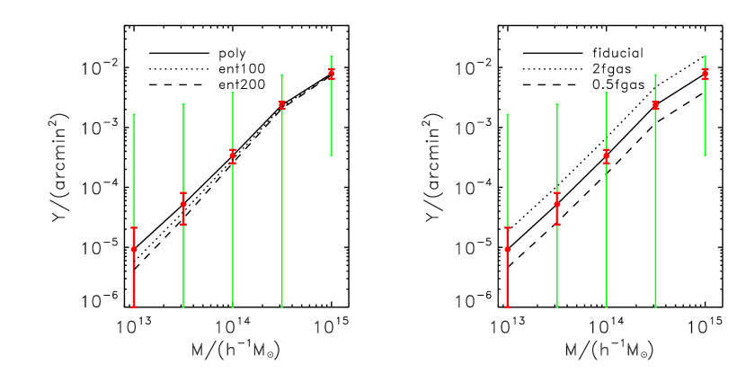
Figure 7: The integrated Compton parameter $Y$ as a function of halo mass. The halo redshifts are set to $z=0.1$. The left panel shows the results assuming different gas equations of state, while the right panel shows the results assuming different gas fraction. The green errorbars represent the 3 $\sigma$ instrument noise of the Planck telescope at 143 GHz, and the red errorbars shows the 3 $\sigma$ error expected from the stack of groups in the corresponding mass range.

With the spatial resolution of Planck, low-mass halos are not spatially resolved, and even the highest mass halos will only be marginally resolved (Aghanim et al., 1997). In this case, observation can only be used to estimate the integrated Compton parameter $Y$ of an entire group (or stack thereof). Fig.7 shows $Y$ as a function of group mass, $M$. Here $Y$ is obtained by integrating $y_{\rm comp}$ within the virial radius of the halo. As discussed in Section 3, for a group with a given mass, $M$, the $Y$-parameter decreases with the redshift of the group. For each mass bin we therefore average $Y$ using the mass and redshift distributions of the groups in GCY07.

To predict the error in a given mass bin, we use the number of groups in the GCY07 (see table 1) under the assumption that the noise for each group is independent of that of other groups. In that case the noise of the stacked signal decreases as $N^{-1/2}$, where $N$ is the number of groups in the stack.

In the left-hand panel of Fig.7, the $Y$ parameter is shown for our 3 different models for the gas equation of state. In all three cases, the $Y$ parameter is almost the same at the high-mass end. For low mass groups, however, the entropy-injection models predict lower values for $Y$. For example, for halos with $M\sim 10^{13}\>h^{-1}\rm M_{\odot}$ the $Y$ value predicted by the polytropic model is larger than that of the Ent200 model by a factor of about two. In the right-hand panel of Fig.7, we show the effect of gas fraction. Here again the results are shown for gas fraction that is 2 and $0.5$ times that adopted in the fiducial model. The larger error bars show the 3 $\sigma$ detection limit for individual halos expected for Planck. The smaller error bars represent the uncertainties in the corresponding stacks of groups. Clearly, by stacking groups of similar masses, the total SZE flux around groups with masses $M\lower 3.01385pt\hbox{$\;\buildrel>\over{\sim}\;$}10^{13.5}\>h^{-1}\rm M_{\odot}$ can be constrained well. In particular, the GCY07 is large enough to constrain the hot gas fractions to an accuracy of $\lower 3.01385pt\hbox{$\;\buildrel<\over{\sim}\;$}40\%$ for groups with masses higher than $10^{13.5}\>h^{-1}\rm M_{\odot}$. However the sensitivity and spatial resolution of Planck is not sufficient to distinguish among the different gas equations of state considered here, at least not when using a group catalogue the size of the GCY07. Larger and deeper optical surveys will be required to reduce the noise to sufficiently low levels. For example, if the number of groups is increased by a factor of 4, the observation will be able to distinguish Ent200 and the fiducial model at $\sim 3\sigma$ confidence level.

6.4 Predictions for the SPT and ACT Surveys

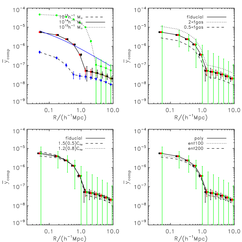
Figure 8: The average Compton parameter $\bar{y}_{\rm comp}$ as a function of the projected halo-centric distance $R$. The top left panel shows the results of the fiducial model for different halo mass. The errorbars show the expected $1\sigma$ uncertainty of the SPT for the corresponding stacks.The expected 1 $\sigma$ uncertainties of observing one single group is shown using blue solid line. The top right panel shows the results assuming different gas fraction. The bottom right panel shows the results assuming different gas equations of state, and the bottom left panel shows the result for different halo concentrations. In these three panels, we adopt a halo mass of $10^{14}\>h^{-1}\rm M_{\odot}$. The results are compared with SPT $1\sigma$ detection limit (green error bars) for a single observation, and the detection limit for stacks (red error bars). We also plot the $1\sigma$ detection limit of ACT(black error bars) for comparison.

In the case of the SPT, the resolution at 150 GHz is 1 arcmin with an instrument sensitivity of 10 $\mu$K/beam. For comparison, the angular sizes corresponding to the virial radii of groups with masses of $10^{13}$, $10^{14}$ and $10^{15}$ $h^{-1}M_{\odot}$ at $z=0.1$ are $5.24$, $11.3$ and $24.3$ arcmin, respectively. Thus, SPT has sufficient spatial resolution to probe the actual hot gas profiles of SDSS groups. However, in order to obtain sufficient S/N, one needs to stack groups of similar masses together, especially at the low mass end. As for Planck, we base our analysis on galaxy groups in the GCY07, even though the area on the sky covered by this group catalogue (obtained from the SDSS DR4) has no overlap with the area covered by the SPT survey (see discussion in Section 5.1). For a group of a given mass at a given redshift, we calculate the SZE profile and smooth it over a one-arcmin scale using a top-hat window. We then average the signal in each mass bin according to the host halo mass distribution given by the SDSS group catalog.

The estimate is made in 11 logarithmic bins of halo-centric distance ($R$), from the halo center to a maximum of $10h^{-1}{\rm Mpc}$. To maximize the S/N, we stack groups in a wide redshift range, from $0.05$ to $0.2$, following the redshift distribution of the GCY07 group catalog. For each $R$-bin, we compute the average signal as

$$\bar{y}_{\rm comp}=\frac{\Sigma_{i}w_{i}y_{i,{\rm comp}}}{\Sigma_{i}w_{i}}\,,$$ (48)

where $y_{i,{\rm comp}}$ is the SZE signal of the $i$th group, and $w_{i}$ is a weighting function chosen to be

$$w_{i}=\frac{1}{D_{i}^{2}}\,,$$ (49)

with $D_{i}$ the angular diameter distance of the $i$th group. This weighting scheme is chosen to account for the fact that for haloes of the same mass, the SZE flux within an annulus of a certain angular distance is inversely proportional to the square of the distance of the halo. The noise of $\bar{y}_{\rm comp}$ in a bin of $R$ is estimated through

$$\sigma_{\rm y}(R)=\sqrt{\frac{\Sigma_{i}w_{i}\,\sigma_{{\rm y},i}^{2}(R)}{\Sigma_{i}w_{i}}}\,,$$ (50)

where $\sigma_{{\rm y},i}(R)$ is the measurement noise of the $i$th group. Assuming that the noise contributions from different beams (i.e., different groups) are independent, we can estimate $\sigma_{{\rm y},i}(R)$ through

$$\sigma_{{\rm y},i}(R)=\frac{\sigma_{\rm m}}{\sqrt{N_{i}(R)}}\,,$$ (51)

where $\sigma_{\rm m}$ is the measurement noise of $\bar{y}_{\rm comp}$ per beam, and $N_{i}(R)$ is the number of beams the annulus contains. Note that $N_{i}(R)$ depends on $i$ because the beam size corresponds to different real space area at different redshifts. The SZE background fluctuation, $\sigma_{\rm bg}$, is estimated as described in Section 5.2, and is added in quadrature to $\sigma_{\rm y}$ to get the total uncertainty

$$\sigma_{\rm tot}=\sqrt{\sigma_{\rm bg}^{2}(R)+\sigma_{\rm y}^{2}(R)}\,.$$ (52)

The upper left-hand panel of Fig.8 shows the average Compton parameter, $\bar{y}_{\rm comp}$, as a function of the projected halo-centric distance $R$ for our fiducial model. Results are shown for the three mass bins around $10^{13}$, $10^{14}$, and $10^{15}\>h^{-1}\rm M_{\odot}$, respectively (see Table 1). The expected $1\sigma$ uncertainties for the stacks of groups are shown with the errorbars. For comparison, the 1-$\sigma$ uncertainty expected from a single group is indicated by the solid blue line. This shows that the SPT can only map the SZE profile of individual halos with masses significantly larger than $10^{14}\>h^{-1}\rm M_{\odot}$. However, by stacking the signal from groups in a catalogue the size of GCY07, one can study the (average) hot gas distribution around halos with masses as low as $\sim 10^{13}h^{-1}{\rm M}_{\odot}$. The remaining three panels of Fig.8 show the predicted, average SZ profile for the stack of GCY07 groups in the $10^{14}\>h^{-1}\rm M_{\odot}$ mass bin for different gas mass fractions (upper right-hand panel), different gas equations of state (lower right-hand panel), and different halo concentrations (lower left-hand panel). Comparing these model predictions with the expected SPT sensitivity, it is clear that SPT can provide stringent constraints on the properties of hot gas in dark matter halos. Even the 2-halo term can be detected with a group catalogue the size of GCY07, allowing one to probe hot gas in the infall regions around group-sized haloes (i.e., possibly associated with the WHIM inside filaments and pancakes).

We also predict the signal and detection limit expected from ACT. The procedure of the calculation is the same as for SPT, except that the predicted signal is now smoothed with a 1.4 arcmin top-hat window to match the resolution of ACT at 148 GHz. Since the signals are binned into relative large annuli, the results expected from ACT and SPT are almost identical, except that the signal-to-noise is slightly lower for ACT. For comparison, we plot the error-bars expected from the ACT in Fig.8. As one can see, ACT is still able to provide constraints on the hot gas fractions in halos with $M\lower 3.01385pt\hbox{$\;\buildrel>\over{\sim}\;$}10^{14}\>h^{-1}\rm M_{\odot}$.

Figure 9: The predicted SZE around galaxies in two different luminosity bins (as indicated by the $r$-band absolute magnitudes in the low two panels). In the upper panels, the predicted $y_{\rm comp}$ parameter is plotted as a function of the projected distance to the galaxy. The SZE is decomposed into a 1-halo central term (dotted lines), a 1-halo satellite term (dashed lines), and a 2-halo term (dash-dotted lines). The total signal is shown by the solid line. The $1\sigma$ expected uncertainties from SPT are shown as the errorbars on solid circles. We also plot the $1\sigma$ confidence level expected from the ACT survey as error-bars on triangles. In the two lower panels, the host halo mass distribution of the galaxies used to obtain the results shown in the upper two panels are shown for central galaxies (solid line) and satellites (dashed line). The distributions are normalized individually. The satellite fraction $f_{\rm sat}$ in each luminosity bin is marked in the respective panel.

Figure 10: The figure shows how the haloes in different mass range contribute to the SZE signal around galaxies that in certain luminosity bins. The absolute magnitude range of galaxies are marked on top right of each subplot. Different linestyles represent contribution from halo of different mass range as shown on top left panel. The unit is in $\>h^{-1}\rm M_{\odot}$

Figure 11: The model dependence of $y_{\rm comp}(R)$ predicted around galaxies in the luminosity bin $[-22,-21.5]$. The $1\sigma$ expected uncertainties from SPT are shown as the errorbars on solid circles. $1\sigma$ detection limit for ACT survey using error bar on triangle. The upper left panel shows the results for different equations of state. The upper right panel shows the results for different gas fractions. The lower left panel shows the results for two different set of cosmological parameters. And the lower right panel shows the effect of changing the halo concentration.

6.4.1 The Impact of Mass Uncertainties

In the analysis presented above, the calculations are made under the assumption that there are no errors in the halo mass assigned to each individual group. However, using mock galaxy redshift surveys, Y07 have shown that the error on the halo mass assigned to an individual group is of the order of 0.2 to 0.3 dex. To test the importantance of these errors, we repeat the same exersize as above, but this time adding a random ‘error’ to the halo mass of each group in the stack, drawn from a log-normal distribution with a rms of 0.2 dex. The ‘perturbed’ masses are then used to calculated the SZE signal. Fig.12 shows a comparison between the results thus obtained with the ‘perturbed’ masses and those obtained assuming the halo masses are perfectly estimated. The difference caused by the mass uncertainties is negligible at large radii (2-halo term). On small scales, where the 1-halo term dominates, the mass errors cause an increase in $y_{\rm comp}$ of about $7\%$, and the 1-halo term now extends to slightly larger radii. This is due to the inclusion of massive halos in the tail of the mass distribution.

In real observation, this effect may be quantified by applying the same analysis to mock group catalogs selected in the same way as the real catalog. Using these mock catalogs, one can estimate the uncertainties in the assigned halo masses, which in turn can be incorporated in the modeling, similar to what we have done here.

Figure 12: The effect of mass assignment errors. The solid line in the left panel shows the original mass distribution in the mass bin $[10^{13.9},10^{14.1}]\>h^{-1}\rm M_{\odot}$ as given by GCY07, while the dashed line shows the distribution including the broadening modeled with a lognormal distribution with a dispersion of 0.2 dex. The right panel shows the results obtained with these two mass distributions.

6.5 The Cross Correlation between Galaxies and the Compton Parameter

Another way to probe the properties of the hot gas in dark matter halos is to study how the hot gas correlates with galaxies of different luminosity. One advantage of such analysis is that the number of galaxies that can be used is large, so that one can stack the SZE signals around many galaxies, thus achieving high signal-to-noise. Even more importantly, measurement of the galaxy-SZE cross correlation does not require a selection of galaxy groups, which always carries some uncertainties and which typically requires spectroscopic redshifts for individual galaxies. In fact, as we demonstrate below, the precision of photometric redshift may be sufficient to obtain reliable measurements of the galaxy-SZE cross correlation. Since photometric redshifts are much easier to obtain than their spectroscopic counterparts, the galaxy-SZE correlation can be used to study the hot gas evolution out to higher redshift. The stacking results can then be interpreted with the CLF discussed in Section 4 The solid lines in the upper two panels of Fig. 9 show $y_{\rm comp}(R)$ around stacks of galaxies with absolute $r$-band magnitudes in the ranges $-20<M_{r}-5\log h\leq-19$ (left-hand panels) and $-21.5<M_{r}-5\log h\leq-22$ (right-hand panels). The dotted, dashed, and dot-dashed curves show the contributions from the 1-halo central, the 1-halo satellite and the 2-halo terms, respectively. These are computed using the method described in Section 4 with the CLF parameters of Cacciato et al. (2009). Errorbars are obtained using the same method as described in Section 6.4, except that rather than using the numbers of galaxy groups in the GCY07, we use the numbers of galaxies in the spectroscopic sample of the SDSS DR4 with absolute $r$-band magnitudes in the respective bins, and with redshifts $0.05\leq z\leq 0.20$. The error-bars are estimated using the total independent angular area of all the angular annuli (corresponding to the bin size in $R$) around all galaxies in the corresponding luminosity bin, in comparison to the SPT (ACT) beam size. The lower panels of Fig. 9 show the host halo mass distributions for central galaxies (solid lines) and satellite galaxies (dashed lines) in the corresponding magnitude bins. For clarity, the distributions are individually normalized, while the satellite fractions in each luminosity bin are indicated in the corresponding panels.

As one can see, the SZE signal for the brighter sample is dominated by different contributions on different scales. The 1-halo central term dominates the signal up to a scale of about $0.3h^{-1}{\rm Mpc}$. On scales of $0.3h^{-1}{\rm Mpc}\lower 3.01385pt\hbox{$\;\buildrel<\over{\sim}\;$}R\lower 3.01385pt\hbox{$\;\buildrel<\over{\sim}\;$}2h^{-1}{\rm Mpc}$ the signal is dominated by the 1-halo satellite term, while the 2-halo term dominates on larger scales. For the fainter sample, the situation is different. Since the host halos of these central galaxies are mostly low mass halos with $10^{11}\>h^{-1}\rm M_{\odot}\lower 3.01385pt\hbox{$\;\buildrel<\over{\sim}\;$}M\lower 3.01385pt\hbox{$\;\buildrel<\over{\sim}\;$}10^{12}$ $\>h^{-1}\rm M_{\odot}$ (see lower left-hand panel), the 1-halo-central term extends only to relatively small scales and never dominates the signal. The 1-halo satellite term dominates the SZ signal from the center out to $\sim 1\>h^{-1}{\rm{Mpc}}$, after which the 2-halo term dominates. This is important, as it indicates that even very accurate measurements of the average $y_{\rm comp}(R)$ around relatively faint galaxies yields virtually no constraints on the properties of hot gas in low mass haloes (i.e., the haloes that host central galaxies of those luminosities). Rather, since the SZ signal scales strongly with halo mass ($Y\propto M^{a}$ with $a\simeq 1.6$), the signal on small scales is dominated by the 1-halo satellites term, even though satellites only make up a relatively small fraction ($\sim 21\%$) of all galaxies in that luminosity bin.

This is also evident from Fig. 10 which shows how galaxies in halos of different masses contribute to the SZE effect. Results are shown for four different luminosity bins, as indicated. In the brightest bin, [-22.5,-21.5], halos in the mass range $10^{13}$ - $10^{14}\,\>h^{-1}\rm M_{\odot}$ dominate the signal in the inner part, while more massive halos only dominate the signal between $0.4$ and $1h^{-1}\>{\rm Mpc}$. This can be understood with the help of Fig.9. From the inner to outer parts, the signal of the brightest bin is first dominated by the 1-halo central term and then by the 1-halo satellite term. Since host halos of satellites on average are more massive than those of central galaxies of the same luminosity, the 1-halo satellite term dominates on intermediate scales. For faint luminosity bins, the SZ signal on small scales ($\lower 3.01385pt\hbox{$\;\buildrel<\over{\sim}\;$}1\>h^{-1}{\rm{Mpc}}$) is always dominated by the most massive halos. Although only a relatively small fraction of faint galaxies reside in these massive halos (as satellites) their contribution to the SZ effect is larger than that from the far more numerous centrals in less massive halos.

Fig. 11 shows the predictions for galaxies in the [-22.5,-21.5] luminosity bin for different gas equations of state (upper left-hand panel), different gas mass fractions (upper right-hand panel), different cosmological parameters (lower left-hand panel), and different halo concentrations (lower right-hand panel). Here again we see that the statistical uncertainties expected from a survey like SPT are much smaller than the differences between different models, indicating that an analysis along these lines can put tight constraints on the hot gas properties in dark matter halos spanning a relatively wide range in masses.

The lower left-hand panel of Fig. 11 shows a comparison between $y_{\rm comp}(R)$ expected around a stack of galaxies in the [-22.5,-21.5] luminosity bin in the WMAP1 and WMAP3 cosmologies (see Table 3 for the corresponding cosmological parameters). In addition to changing the cosmological parameters here we have also changed the CLF that is used to predict $y_{\rm comp}(R)$. For each cosmology, the best-fit CLF parameters have been obtained by Cacciato et al. (2009) using the combined constraints from the observed galaxy luminosity function, the luminosity dependence of galaxy clustering, and the SDSS group catalogue of Yang et al. (2007). As shown in Cacciato et al. (2009), both models fit the observed abundance and clustering of galaxies equally well. However, whereas the WMAP3 model simultaneously matches the galaxy-galaxy lensing data of Mandelbaum et al. (2006), the WMAP1 clearly overpredicts the lensing signal (i.e., the WMAP1 model predicts mass-to-light ratios that are too high). Hence, galaxy-galaxy lensing can be used to break the degeneracy between cosmology and halo occupation statistics (see also Yang et al., 2006; Li et al., 2009). Interestingly, the results presented here suggest that the cross correlation between galaxies and the Compton parameter can also be used to discriminate between these different models. However, it is clear from Fig. 11 that a change in cosmological parameters has a similar effect as a change in the hot gas fraction or a change in halo concentration. Hence, it will be important to have precise constraints on cosmological parameters in order to use the galaxy-Compton parameter cross correlation to constrain the properties of hot halo gas. The precision of upcoming CMB observations, such as Planck, will be able to pin down all important cosmological parameters to very high accuracy, making the SZE analysis presented here a powerful tool to study the gas distribution in dark matter halos.

Finally, for comparison, we also plot the error-bars expected from the ACT survey. Clearly, the uncertainties in ACT are slightly larger than that of SPT and can also tightly constrain the properties of the hot gas in halos that host these galaxies.

6.5.1 Photometric Redshifts

When calculating the cross-correlation between galaxies and hot gas, we have assumed that the redshifts of the galaxies have no errors. Although this is a reasonable assumption to make when using spectroscopic surveys, we now investigate how significantly redshift errors, such as those present in a photometric redshift survey, impact on the analysis. Redshift errors introduce errors in both the absolute magnitudes (luminosities) and the projected distances. In order to estimate the resulting impact on $y_{\rm comp}(R)$ we add a redshift error (and its associated luminosity error) to each galaxy in the $[-21.5,-22]$ luminosity bin of the SDSS DR4 catalog, using a Gaussian distribution with standard deviations of $(1+z)\times 5\%$ and $(1+z)\times 3\%$. This roughly mimics the redshift errors expected from future photometric surveys, such as the LSST. Next we compute the galaxy-Compton parameter cross correlation using the new redshifts. Results are shown in Fig. 13. The change in the cross correlation due to photo-z errors of 5% (3%) is negligible at small radii, but increases to $\sim 20\%$ ($\sim 10\%$) at $1-2$ $h^{-1}Mpc$. We also find that, if one can exclude the 20 percentile of the galaxies with the largest redshift errors, the measurement errors caused by the photo-$z$ errors shrink to about half this value. This suggests that the cross correlation analysis considered here can be extended to photometric surveys, but that precise modeling of the galaxy-Compton parameter cross correlation may require some treatment of the photo-$z$ error distribution.

Figure 13: This figure shows how the photo-$z$ error affects the observed $y_{\rm comp}$. The solid line shows the Compton parameter $y_{\rm comp}(R)$ in the luminosity bin [-22,-21.5]. The dashed and dotted lines show the results of the calculations that include a photo-$z$ error of $5\%$ and $3\%$ in (1+z), respectively.

6.6 Model based on observed X-ray gas profile

In previous sections, the hot gas profile is modeled based on the assumption of hydrostatic equilibrium between the hot gas and the dark matter halo. This model is roughly consistent with the observed X-ray luminoisty and gas fraction of galaxy clusters (e.g. Moodley et al., 2008). However, recent work by Komatsu et al. (2010) showed that the gas profile thus derived is different from that derived from X-ray observation (Arnaud et al., 2010, A10, hereafter). Since our fiducial model is very similar to the KS model (see Section 2.2.2), there is the same uncertainty due to the assumed hot gas density profile.

In Fig.14, we compare our hot gas pressure profile with that derived from A10, with the latter obtained using the formula given in the Appendix of Komatsu et al. (2010). The horizontal axis is scaled by $R_{500}$, the radii within which the mean density is 500 times the critical density. As in Komatsu et al. (2010), we also find that the pressure profile predicted by our model is flatter and more extended. This difference causes a significant difference in the predicted SZE at large radii.

One possibility to alleviate the tension between the two models is to change the gas fraction and boundary condition in our model. In our model, the boundary condition is set by $T(r_{\rm vir})=T_{\rm vir}$, but X-ray observations indicate that the temperature drops more rapidly in the outer part of the halo. For some halo massed, the slope of the X-ray derived pressure profile can be fitted by decreasing the temperature at virial radius. However, in hydrostatic equilibrium the low boundary temperature results in a higher inner gas density, and the amplitude of SZE at small scales becomes higher than that based on X-ray observations. For a halo of $10^{14}\>h^{-1}\rm M_{\odot}$, we can decrease the discrepancy between our fiducial profile and X-ray profile by setting $T(r_{\rm vir})=0.3T_{\rm vir}$ and the gas to total fraction $f_{\rm gas}=0.08$. However, we cannot find a single boundary condition that can fit the X-ray profile for all halo masses. Because of these uncertainties, the boundary condition should be treated as a free parameter when studying the hot gas properties of groups with future SZE observation.

Observationally, X-ray observations lack the sensitivity to reliably probe hot gas beyond $R_{500}$, because the X-ray luminosity scales with the square of the gas density. In A09, the pressure profile is derived using REXCESS data (Böhringer et al., 2007), where X-ray measurements are limited within $R_{500}$. Thus, the pressure profile at larger radii is still uncertain.

In order to test how the uncertainties in the hot gas pressure profile affect our prediction of the SZE, we compare in Fig.15 the cross-correlation between the SZE and galaxies predicted by our fiducial model with that predicted by the X-ray observation-based model. The predictions of our fiducial model is a factor of 2 to 3 larger. This indicates that the observation of the cross-correlation between SZE and galaxies can be used to distinguish these two models.

Figure 14: The hot gas profile of our fiducial model (solid lines) in comparison with that derived in (Arnaud et al., 2010) (dashed lines). The upper panel shows the hot gas pressure profile as a function of radius. The bottom panel shows the Compton $y$-parameter profile. In each panel, the upper set of lines are for the halo of $10^{14}\>h^{-1}\rm M_{\odot}$ and the lower set of lines for halo of $10^{13}\>h^{-1}\rm M_{\odot}$. The horizontal axis shows radii scaled by the corresponding $R_{500}$.

Figure 15: The $y_{\rm comp}(R)$ around galaxies in luminosity bins $[-22,-21.5]$ (left) and $[-20,-19]$ (right) predicted by our fiducial model (solid lines) in comparison with that predicted with the formula derived from (Arnaud et al., 2010) (dashed lines).

7 Conclusions

In this paper we have used simplified models to demonstrate the potential of using the SZE to probe the hot gas expected to be associated with dark matter halos. We have shown that by stacking SZE maps expected from the Planck, ACT and/or SPT surveys, one can probe the hot gas properties in galaxy groups with halo masses down to $\sim 10^{13}\>h^{-1}\rm M_{\odot}$. The SZE for halos with similar masses are examined in terms of halo models. Splitting the total SZE signal into 1-halo and 2-halo terms, we have shown that in high-mass halos the 1-halo term dominates the signal within the virial radius; in low-mass halos the 2-halo term is also significant on small scales. The model predictions are sensitive to the amount of hot gas assumed to be in halos, and our results show that a SPT-like survey can provide a stringent constraint on the hot gas fraction for halos with masses $M\lower 3.01385pt\hbox{$\;\buildrel>\over{\sim}\;$}10^{13}\>h^{-1}\rm M_{\odot}$. Furthermore, such observations can also provide stringent constraints on the equation of state of the hot gas as well as the concentrations of dark matter halos.

Using WMAP-7-year data, Komatsu et al. (2010) stacked clusters in X-ray catalog and compared the resulting SZE profile with the prediction of the KS model(Komatsu & Seljak, 2001) that uses a polytropic gas equation of state very similar to the polytropic model considered here. They found that this model over-predicts the SZE by a factor of 1.5 to 2. In a recent study using SPT data, Lueker et al. (2009) also found that the observed SZE power spectrum is lower than that expected from polytropic model. However, as we have shown above, entropy injection can reduce the amplitude of the SZE by a factor of 1.5 at the inner parts of halos with masses $10^{14}\>h^{-1}\rm M_{\odot}$, suggesting that non-gravitational heating may have played an important role.

We have also explored the idea of using the cross correlation between hot gas and galaxies of different luminosity to probe the hot gas in dark matter halos with the use of the CLF. Since the number of galaxies that can be used is large, especially in the forthcoming large photometric surveys where accurate photometric redshifts of individual galaxies can be obtained, the measurement can be made to high precision. Our results show that, with the help of CLF modeling, one can constrain the hot gas profile in halos with masses down to $10^{13}\>h^{-1}\rm M_{\odot}$. Cosmological parameters, especially the value of $\sigma_{8}$, can affect galaxy - hot gas cross-correlation. Thus, in order to use the observed SZE to constrain the hot gas properties in dark matter halos, precise constraints on cosmological parameters are required.

In summary, the upcoming SZE surveys are expected to provide an important avenue to study the hot gas properties in dark matter halos. Combining with large optical galaxy surveys and using the stacking method proposed here, the SZE to be observed in forthcoming surveys will allow us to study in great detail the hot gas properties in galaxy groups where most galaxies reside. This, in turn, will shed new light on how galaxy form and evolve in dark matter halos.

Appendix A Angular power spectrum and SZE map

We write the SZE power spectrum, $P_{\rm sz}(k,z)$, as

$$P_{\rm sz}(k,z)=P_{\rm sz}^{\rm 1h}(k,z)+P_{\rm sz}^{\rm 2h}(k,z)\,,$$ (53)

where the 1-halo contribution is

$$P_{\rm sz}^{\rm 1h}(k,z)=I^{2}_{1,\rm sz}(k,z),$$ (54)

and the 2-halo contribution is

$$P_{\rm sz}^{\rm 2h}(k,z)=P_{\rm lin}(k,z)I_{2,\rm sz}^{2}\,.$$ (55)

Here

$$I_{1,\rm sz}^{2}(k,z)=\int_{M_{\rm min}}^{M_{\rm max}}n(M,z)\,{\tilde{u}}_{p}^{2}(k|M,z)\,{\rm d}M\,.$$ (56)

and

$$I_{2,\rm sz}(k,z)=\int_{M_{\rm min}}^{M_{\rm max}}n(M,z)\,{\tilde{u}}_{p}(k|M,z)\,b(M,z)\,{\rm d}M\,.$$ (57)

Observationally, one typically measures the angular power spectrum, which is the integration of the power spectrum along the line-of-sight. To derive the angular power spectrum, we expand the CMB temperature fluctuations due to the SZE in spherical harmonics:

$$\frac{\Delta T}{T_{{\rm CMB}}}(\hat{\bf n})=\sum_{lm}\left(\frac{\Delta T}{T_{{\rm CMB}}}\right)_{lm}Y_{lm}(\hat{\bf n})$$ (58)

The angular power spectrum can then be written as:

$$\left\langle\left(\frac{\Delta T}{T_{\rm CMB}}\right)_{lm}\left(\frac{\Delta T}{T_{\rm CMB}}\right)_{l^{\prime}m^{\prime}}\right\rangle=C_{l}^{\rm sz}\delta_{ll^{\prime}}\delta_{mm^{\prime}}\,.$$ (59)

Using the Limber approximation (Limber, 1953), we have

$$C_{l}^{\rm sz}=\int^{z_{\rm max}}_{z_{\rm min}}dz\frac{{\rm d}^{2}V}{{\rm d}z{\rm d}\Omega}P_{l,\rm sz}(l,z)\,,$$ (60)

where ${\rm d}^{2}V/{\rm d}z{\rm d}\Omega$ is the comoving volume per unit redshift per unit solid angle, and the projected power spectrum, $P_{l,\rm sz}(l,z)$, is related to the 3-dimensional power spectrum via

$$P_{l,\rm sz}(l,z)=\left[\frac{W_{\rm sz}(z)}{D_{\rm c}(z)}\right]^{2}\,\left[I_{1,\rm sz}^{2}(l,z)+I_{2,\rm sz}^{2}(l,z)\right]\,,$$ (61)

with

$$W_{\rm sz}(z)=\Theta_{\nu}\frac{\sigma_{T}}{m_{\rm e}}\frac{k_{\rm B}}{a^{2}(z)}\,.$$ (62)

Here $D_{\rm c}(z)$ is the comoving distance from redshift $z$, and $a(z)$ is the scale factor.

We carry out the integration using Eq.(60) from redshift $z_{\rm min}=0$ to $z_{\rm max}=5$. For the mass limits, we use $M_{\rm min}=5\times 10^{11}\>h^{-1}\rm M_{\odot}$ and $M_{\rm max}=5\times 10^{15}\>h^{-1}\rm M_{\odot}$. We then use the angular power-spectrum as an input to the synfast subroutine in the HEALPIX package (Górski et al., 2005) in order to generate an all sky SZE map. In Fig.16, we show the standard deviation of the background SZE flux measured within an angular radius $\theta$ (solid line) and compare it with the instrumental noise levels of SPT, ACT and Planck. The background noise is much smaller than the instrumental noise. We also compare our result with the fitting formula given by Shaw et al. (2008) (dotted line) who use the background SZE noise measured from a light cone simulation with cosmological parameters similar to ours. Note the good agreement between the two.

Figure 16: The fluctuation of the SZE background as a function of angular radius $\theta$. The solid line shows our result, and the dotted line shows the fitting formula of Shaw et al. (2008). The triangles show the instrumental noise levels of SPT (150GHz), ACT triangles show the instrumental noise levels of SPT (143GHz), ACT (148 GHz) and Planck (150GHz), respectively.

References

- Adelman-McCarthy et al. (2006) Adelman-McCarthy J. K., Agüeros M. A., Allam S. S., Anderson K. S. J., Anderson S. F., Annis J., Bahcall N. A., Baldry 2006, ApJS, 162, 38
- Aghanim et al. (1997) Aghanim N., de Luca A., Bouchet F. R., Gispert R., Puget J. L., 1997, A&A, 325, 9
- Arnaud et al. (2010) Arnaud M., Pratt G. W., Piffaretti R., Böhringer H., Croston J. H., Pointecouteau E., 2010, A&A, 517, A92+
- Ascasibar et al. (2003) Ascasibar Y., Yepes G., Müller V., Gottlöber S., 2003, MNRAS, 346, 731
- Bartelmann (2001) Bartelmann M., 2001, A&A, 370, 754
- Bartlett (2006) Bartlett J. G., 2006, ArXiv Astrophysics e-prints
- Berlind et al. (2006) Berlind A. A., Frieman J., Weinberg D. H., Blanton M. R., Warren M. S., Abazajian K., Scranton R., Hogg 2006, ApJS, 167, 1
- Birkinshaw (1999) Birkinshaw M., 1999, PhR, 310, 97
- Birkinshaw et al. (1978) Birkinshaw M., Gull S. F., Northover K. J. E., 1978, MNRAS, 185, 245
- Böhringer et al. (2007) Böhringer H., Schuecker P., Pratt G. W., Arnaud M., Ponman T. J., Croston J. H., Borgani S. a., 2007, A&A, 469, 363
- Borgani et al. (2004) Borgani S., Murante G., Springel V., Diaferio A., Dolag K., Moscardini L., Tormen G., Tornatore L., Tozzi P., 2004, MNRAS, 348, 1078
- Bryan & Norman (1998) Bryan G. L., Norman M. L., 1998, ApJ, 495, 80
- Bullock et al. (2001) Bullock J. S., Kolatt T. S., Sigad Y., Somerville R. S., Kravtsov A. V., Klypin A. A., Primack J. R., Dekel A., 2001, MNRAS, 321, 559
- Cacciato et al. (2009) Cacciato M., van den Bosch F. C., More S., Li R., Mo H. J., Yang X., 2009, MNRAS, 394, 929
- Colless et al. (2001) Colless M., Dalton G., Maddox S., Sutherland W., Norberg P., Cole S., Bland-Hawthorn J., Bridges 2001, MNRAS, 328, 1039
- Comerford & Natarajan (2007) Comerford J. M., Natarajan P., 2007, MNRAS, 379, 190
- Cooray (2006) Cooray A., 2006, MNRAS, 365, 842
- Dolag et al. (2004) Dolag K., Bartelmann M., Perrotta F., Baccigalupi C., Moscardini L., Meneghetti M., Tormen G., 2004, A&A, 416, 853
- Eke et al. (2001) Eke V. R., Navarro J. F., Steinmetz M., 2001, ApJ, 554, 114
- Evrard et al. (1996) Evrard A. E., Metzler C. A., Navarro J. F., 1996, ApJ, 469, 494
- Finoguenov et al. (2007) Finoguenov A., Ponman T. J., Osmond J. P. F., Zimer M., 2007, MNRAS, 374, 737
- Frenk et al. (1999) Frenk C. S., White S. D. M., Bode P., Bond J. R., Bryan G. L., Cen R., Couchman H. M. P., 1999, ApJ, 525, 554
- Górski et al. (2005) Górski K. M., Hivon E., Banday A. J., Wandelt B. D., Hansen F. K., Reinecke M., Bartelmann M., 2005, ApJ, 622, 759
- Goto (2005) Goto T., 2005, MNRAS, 359, 1415
- Grego et al. (2001) Grego L., Carlstrom J. E., Reese E. D., Holder G. P., Holzapfel W. L., Joy M. K., Mohr J. J., Patel S., 2001, ApJ, 552, 2
- Guzik & Seljak (2002) Guzik J., Seljak U., 2002, MNRAS, 335, 311
- Hall et al. (2010) Hall N. R., Keisler R., Knox L., Reichardt C. L., Ade P. A. R., Aird K. A., Benson B. A., Bleem L. E. a., 2010, ApJ, 718, 632
- Hallman et al. (2007) Hallman E. J., O’Shea B. W., Burns J. O., Norman M. L., Harkness R., Wagner R., 2007, ApJ, 671, 27
- Hernández-Monteagudo et al. (2004) Hernández-Monteagudo C., Genova-Santos R., Atrio-Barandela F., 2004, ApJL, 613, L89
- Hernández-Monteagudo et al. (2006) Hernández-Monteagudo C., Trac H., Verde L., Jimenez R., 2006, ApJL, 652, L1
- Ho et al. (2009) Ho S., Dedeo S., Spergel D., 2009, ArXiv e-prints
- Holder & Carlstrom (2001) Holder G. P., Carlstrom J. E., 2001, ApJ, 558, 515
- Jing (2000) Jing Y. P., 2000, ApJ, 535, 30
- Jing & Suto (2000) Jing Y. P., Suto Y., 2000, ApJ, 529, L69
- Koester et al. (2007) Koester B. P., McKay T. A., Annis J., Wechsler R. H., Evrard A., Bleem L., Becker M., Johnston D., 2007, ApJ, 660, 239
- Komatsu & Seljak (2001) Komatsu E., Seljak U., 2001, MNRAS, 327, 1353
- Komatsu et al. (2010) Komatsu E., Smith K. M., Dunkley J., Bennett C. L., Gold B., Hinshaw G., Jarosik N., Larson D., 2010, ArXiv e-prints
- LaRoque et al. (2006) LaRoque S. J., Bonamente M., Carlstrom J. E., Joy M. K., Nagai D., Reese E. D., Dawson K. S., 2006, ApJ, 652, 917
- Lewis et al. (2000) Lewis G. F., Babul A., Katz N., Quinn T., Hernquist L., Weinberg D. H., 2000, ApJ, 536, 623
- Li et al. (2009) Li R., Mo H. J., Fan Z., Cacciato M., van den Bosch F. C., Yang X., More S., 2009, MNRAS, 394, 1016
- Limber (1953) Limber D. N., 1953, ApJ, 117, 134
- Lloyd-Davies et al. (2000) Lloyd-Davies E. J., Ponman T. J., Cannon D. B., 2000, MNRAS, 315, 689
- Lueker et al. (2009) Lueker M., Reichardt C. L., Schaffer K. K., Zahn O., Ade P. A. R., Aird K. A., Benson B. A., Bleem L. E., 2009, ArXiv e-prints
- Macciò et al. (2007) Macciò A. V., Dutton A. A., van den Bosch F. C., Moore B., Potter D., Stadel J., 2007, MNRAS, 378, 55
- Mandelbaum et al. (2006) Mandelbaum R., Seljak U., Kauffmann G., Hirata C. M., Brinkmann J., 2006, MNRAS, 368, 715
- Mather et al. (1999) Mather J. C., Fixsen D. J., Shafer R. A., Mosier C., Wilkinson D. T., 1999, ApJ, 512, 511
- Milkeraitis et al. (2010) Milkeraitis M., van Waerbeke L., Heymans C., Hildebrandt H., Dietrich J. P., Erben T., 2010, MNRAS, pp 701–+
- Miller et al. (2005) Miller C. J., Nichol R. C., Reichart D., Wechsler R. H., Evrard A. E., Annis J., McKay T. A., Bahcall N. A., Bernardi M., Boehringer H., Connolly A. J., Goto T., Kniazev A., Lamb D., Postman M., Schneider D. P., Sheth R. K., Voges W., 2005, AJ, 130, 968
- Mo & White (1996) Mo H. J., White S. D. M., 1996, MNRAS, 282, 347
- Moodley et al. (2008) Moodley K., Warne R., Goheer N., Trac H., 2008, ArXiv e-prints
- More et al. (2009) More S., van den Bosch F. C., Cacciato M., Mo H. J., Yang X., Li R., 2009, MNRAS, 392, 801
- More et al. (2010) More S., van den Bosch F. C., Cacciato M., Skibba R., Mo H. J., Yang X., 2010, ArXiv e-prints
- Muchovej et al. (2007) Muchovej S., Mroczkowski T., Carlstrom J. E., Cartwright J., Greer C., Hennessy R., Loh M., Pryke C., Reddall B., Runyan M., Sharp M., Hawkins D., Lamb J. W., Woody D., Joy M., Leitch E. M., Miller A. D., 2007, ApJ, 663, 708
- Myers et al. (1997) Myers S. T., Baker J. E., Readhead A. C. S., Leitch E. M., Herbig T., 1997, ApJ, 485, 1
- Navarro et al. (1997) Navarro J. F., Frenk C. S., White S. D. M., 1997, ApJ, 490, 493
- Nord et al. (2009) Nord M., Basu K., Pacaud F., Ade P. A. R., Bender A. N., Benson B. A., Bertoldi F., Cho H., 2009, ArXiv e-prints
- Oguri et al. (2009) Oguri M., Hennawi J. F., Gladders M. D., Dahle H., Natarajan P., Dalal N., Koester B. P., Sharon K., Bayliss M., 2009, ApJ, 699, 1038
- Ostriker et al. (2005) Ostriker J. P., Bode P., Babul A., 2005, ApJ, 634, 964
- Plagge et al. (2010) Plagge T., Benson B. A., Ade P. A. R., Aird K. A., Bleem L. E., Carlstrom J. E., Chang C. L. a., 2010, ApJ, 716, 1118
- Ponman et al. (1999) Ponman T. J., Cannon D. B., Navarro J. F., 1999, Nature, 397, 135
- Press & Schechter (1974) Press W. H., Schechter P., 1974, ApJ, 187, 425
- Rasia et al. (2004) Rasia E., Tormen G., Moscardini L., 2004, MNRAS, 351, 237
- Sealfon et al. (2006) Sealfon C., Verde L., Jimenez R., 2006, ApJ, 649, 118
- Shaw et al. (2008) Shaw L. D., Holder G. P., Bode P., 2008, ApJ, 686, 206
- Sheth et al. (2001) Sheth R. K., Mo H. J., Tormen G., 2001, MNRAS, 323, 1
- Spergel et al. (2007) Spergel D. N., Bean R., Doré O., Nolta M. R., Bennett C. L., Dunkley J., Hinshaw G., Jarosik N., 2007, ApJS, 170, 377
- Staniszewski et al. (2009) Staniszewski Z., Ade P. A. R., Aird K. A., Benson B. A., Bleem L. E., Carlstrom J. E., Chang C. L., Cho 2009, ApJ, 701, 32
- Sunyaev & Zeldovich (1972) Sunyaev R. A., Zeldovich Y. B., 1972, Comments on Astrophysics and Space Physics, 4, 173
- Swetz (2009) Swetz D. S., 2009, PhD thesis, University of Pennsylvania
- Thomas et al. (2001) Thomas P. A., Muanwong O., Pearce F. R., Couchman H. M. P., Edge A. C., Jenkins A., Onuora L., 2001, MNRAS, 324, 450
- Turner (2002) Turner C., 2002, APS Meeting Abstracts, pp 16007–+
- Umetsu et al. (2009) Umetsu K., Birkinshaw M., Liu G.-C., Wu J.-H. P., Medezinski E., Broadhurst T., Lemze D., Zitrin A., 2009, ApJ, 694, 1643
- van den Bosch et al. (2004) van den Bosch F. C., Norberg P., Mo H. J., Yang X., 2004, MNRAS, 352, 1302
- van den Bosch et al. (2003) van den Bosch F. C., Yang X., Mo H. J., 2003, MNRAS, 340, 771
- van den Bosch et al. (2007) van den Bosch F. C., Yang X., Mo H. J., Weinmann S. M., Macciò A. V., More S., Cacciato M., Skibba R., Kang X., 2007, MNRAS, 376, 841
- Vikhlinin et al. (2006) Vikhlinin A., Kravtsov A., Forman W., Jones C., Markevitch M., Murray S. S., Van Speybroeck L., 2006, ApJ, 640, 691
- Voit et al. (2002) Voit G. M., Bryan G. L., Balogh M. L., Bower R. G., 2002, ApJ, 576, 601
- White & Majumdar (2004) White M., Majumdar S., 2004, ApJ, 602, 565
- Yang et al. (2005) Yang X., Mo H. J., Jing Y. P., van den Bosch F. C., 2005, MNRAS, 358, 217
- Yang et al. (2003) Yang X., Mo H. J., van den Bosch F. C., 2003, MNRAS, 339, 1057
- Yang et al. (2008) Yang X., Mo H. J., van den Bosch F. C., 2008, ApJ, 676, 248
- Yang et al. (2005) Yang X., Mo H. J., van den Bosch F. C., Jing Y. P., 2005, MNRAS, 356, 1293
- Yang et al. (2006) Yang X., Mo H. J., van den Bosch F. C., Jing Y. P., Weinmann S. M., Meneghetti M., 2006, MNRAS, 373, 1159
- Yang et al. (2007) Yang X., Mo H. J., van den Bosch F. C., Pasquali A., Li C., Barden M., 2007, ApJ, 671, 153
- York et al. (2000) York D. G., Adelman J., Anderson Jr. J. E., Anderson S. F., Annis J., Bahcall N. A., Bakken J. A., Barkhouser R., 2000, AJ, 120, 1579
- Yoshikawa et al. (2000) Yoshikawa K., Jing Y. P., Suto Y., 2000, ApJ, 535, 593
- Zhao et al. (2003) Zhao D. H., Jing Y. P., Mo H. J., Börner G., 2003, ApJL, 597, L9
- Zhao et al. (2009) Zhao D. H., Jing Y. P., Mo H. J., Börner G., 2009, ApJ, 707, 354