Order-dependent mappings: strong coupling behaviour from
weak coupling expansions in non–Hermitian theories

Abstract

A long time ago, it has been conjectured that a Hamiltonian with a potential of the form $x^{2}+ivx^{3}$, $v$ real, has a real spectrum. This conjecture has been generalized to a class of so-called $\mathcal{PT}\,$symmetric Hamiltonians and some proofs have been given. Here, we show by numerical investigation that the divergent perturbation series can be summed efficiently by an order-dependent mapping (ODM) in the whole complex plane of the coupling parameter $v^{2}$, and that some information about the location of level crossing singularities can be obtained in this way. Furthermore, we discuss to which accuracy the strong-coupling limit can be obtained from the initially weak-coupling perturbative expansion, by the ODM summation method. The basic idea of the ODM summation method is the notion of order-dependent “local” disk of convergence and analytic continuation by an order-dependent mapping of the domain of analyticity augmented by the local disk of convergence onto a circle. In the limit of vanishing local radius of convergence, which is the limit of high transformation order, convergence is demonstrated both by numerical evidence as well as by analytic estimates.

I Introduction

The order-dependent mapping (ODM) summation method has been introduced in Ref. rsezzin and initially applied to series expansions of an integral whose perturbative expansion counts the number of Feynman diagrams with four-point vertices, to the quartic anharmonic oscillator, and to renormalization group (RG) functions in the three-dimensional $\phi^{4}$ quantum field theory rsezzin ; rZJODM . Later, other examples of quantum mechanics and field theory type have been studied rLGZJ ; rRGZJ ; rJLKMPRR ; rKPR ; rKPRS . Some convergence proofs have been given in Refs. rDuJo ; rRGKKHS . However, these examples have in common, as a starting point, perturbations of Hermitian quantum Hamiltonians. In most of them the ODM summation method appears as a higher order extension of some variational calculation rsezzin ; rWECas . Therefore, we may wonder whether Hermiticity plays a role in explaining some specific convergence properties of the method.

Here, we thus consider a non-Hermitian example, the expansion generated by an $\mathrm{i}\,x^{3}$ addition to the harmonic potential. The corresponding Hamiltonian is $\mathcal{PT}\,$symmetric, that is, symmetric under a simultaneous complex conjugation and space reflection. Even though this is not quite obvious, such a Hamiltonian has a real spectrum, as first conjectured by Bessis and Zinn-Justin (1992) and proven in rDDB ; rshin . In this note, we show numerically that the ODM method, suitably adapted to the problem, allows a precise determination of the ground state energy. The convergence properties also give some information about the analyticity as a function of the strength of the $\mathrm{i}\,x^{3}$ perturbation, in particular excluding level crossing in some region of the Riemann surface.

Another potential application of the method is the $\mathrm{i}\phi^{3}$ quantum field theory in two and three space dimensions, whose renormalization group functions describe the Lee–Yang edge singularity of Ising-like statistical models rLYFisher ; rBBJ , should longer perturbative series become available.

II The imaginary cubic potential

We here consider the spectrum of the simplest example of a $\mathcal{PT}\,$symmetric Hamiltonian,

$$H=-\frac{1}{2}\,\frac{\mathrm{d}^{2}}{\mathrm{d}x^{2}}+\frac{1}{2}\,x^{2}+\tfrac{\mathrm{i}}{6}\,\sqrt{g}\;x^{3}\,,$$ (1)

where $g$ is a real positive parameter. Indeed, the Hamiltonian is invariant under simultaneous complex conjugation and parity transformation $x\mapsto-x$. In this convention, the resonance energies of the cubic potential have their branch cut along the negative real $g$ axis, where the quantity $\mathrm{i}\,\sqrt{g}$ becomes real and the particle may tunnel through the “cubic wall” of the potential. One then verifies that the perturbative expansion of the energy eigenvalues $E_{n}$ for $g\to 0$ contains only integer powers of $g$:

$$E_{n}(g)=\sum_{k=0}^{\infty}E_{n,k}g^{k}$$ (2)

with real coefficients. Moreover, a steepest descent calculation of the path integral representation of the corresponding quantum partition function rLOBLip ; rLOBgen ; rZJLOreport yields a large order behaviour of the form

$$E_{n,k}\mathop{\sim}_{k\to\infty}C\;(-1)^{k}\,k^{b}\,A^{-k}\,k!\,,$$ (3)

where $A=24/5$ is the instanton action. The constant $C$ and the half-integer $b$ depend on $n$. The series is divergent for all $g$ and when the expansion parameter is not small, a summation of the perturbative expansion is indispensable. Note that the sign oscillation with $k$ and some additional considerations already suggest that the series is Borel summable (a property proved in rCGM ) and thus that the spectrum, beyond perturbation theory, is real. This was initially the origin of the conjecture of Bessis and Zinn-Justin, which was generalized to other $\mathcal{PT}\,$symmetric Hamiltonians rBeBo ; rBBrJ ; rCMBender . More recently, Padé summability was also rigorously established rVGMMAM . This proof confirms numerical investigations based on the summation of the perturbative expansion by Padé approximants rBeWe . Distributional Borel summability of the perturbation series to the complex resonance energies for negative coupling $g$ was proved in rCaliceti .

In this note, we show by a combination of numerical and analytic arguments that the ODM method is especially well adapted to summing the perturbative series, converging for all values of the expansion parameter in the complex plane and, in addition, in a region of the second sheet of the Riemann surface. It thus also provides additional information about the spectrum for $g$ complex on the Riemann surface rHKWJ .

However, before dealing with the quantum mechanics example, as a warm-up exercise, we first consider the simple integral

$$Z(g)=\frac{1}{\sqrt{2\pi}}\int_{-\infty}^{+\infty}\mathrm{d}x\,\exp\left(-\tfrac{1}{2}x^{2}-\tfrac{\mathrm{i}}{6}\sqrt{g}x^{3}\right),$$ (4)

whose expansion coefficients count the number of Feynman diagrams that appear in the expansion of the partition function $\mathrm{tr}\mathrm{e}^{-\beta H}$ corresponding to the Hamiltonian (1).

Figure 1: Mapping: example of a function analytic in a cut-plane. The cut in the $g$-plane (l.h.s.) is mapped onto the contour $\bar{\Gamma}$ of the $\lambda$-plane (r.h.s.).

III Order-dependent mapping summation method

III.1 Method

The ODM summation method rsezzin is based on some a priori knowledge, or educated guess, of the analytic properties of the function that is expanded. It applies both to convergent and divergent series, although it is mainly useful in the latter case rsezzin .

Let $E(g)$ be an analytic function that has the Taylor series expansion

$$E(g)=\sum_{\ell=0}^{\infty}E_{\ell}\,g^{\ell}\,,$$ (5)

where the equality has to be understood in the sense of a (possibly asymptotic) series expansion. In what follows, we consider two functions analytic at least in a sector (as in the example of Fig. 1) and only mappings $g\mapsto\lambda$ of the form

$$g=\rho\;\frac{\lambda}{(1-\lambda)^{\alpha}}\,,\qquad\alpha>1\,,$$ (6)

where $\alpha$ has to be chosen in accordance with the analytic properties of the function $E$ (a rational number in our examples) and $\rho$ is an adjustable parameter. A general discussion of the method can be found in Refs. rsezzin ; rZJODM . An important property that singles out such a mapping is the following: inverting the mapping, one finds that, for $g\to\infty$, $\lambda$ approaches unity, and $g^{-1/\alpha}$ has a regular expansion in powers of $1-\lambda$ (see the Appendix).

After the mapping (6), $E$ is given by a Taylor series in $\lambda$ of the form

$$E\bigl{(}g(\lambda)\bigr{)}=\sum_{\ell=0}^{\infty}P_{\ell}(\rho)\;\lambda^{\ell},$$ (7)

where the coefficients $P_{\ell}(\rho)$ are polynomials of degree $\ell$ in $\rho$. Since the result is formally independent of the parameter $\rho$, the parameter can be chosen freely. At $\rho$ fixed, the series in $\lambda$ is still divergent, but it has been verified on a number of examples (all Borel summable), and proved in certain cases rDuJo ; rRGKKHS that, by adjusting $\rho$ order by order, one can devise a convergent algorithm. The basic idea is that $\rho$ characterizes a “local radius of convergence” of the divergent input series. As the order of the mapping is increased, $\rho\to 0$. However, the mapping $g=g(\rho,\lambda)$ is constructed so that the circle of convergence of order-dependent radius $\rho$ is always mapped onto a finite domain of the $\lambda$ complex plane.

At a risk of some oversimplification, we can describe the general paradigm of the ODM summation as follows: One “pretends” that the divergent input series is in fact a convergent series, but with a circle of convergence whose radius gradually vanishes as the order of the perturbative expansion is increased. Since both $\rho\to 0$ and also $|\lambda|<1$, the direct expansion in $\lambda$, with variable $\rho$, may then lead to a convergent output series even for large $g$.

The $k$-th approximant $E^{(k)}(g)$ is constructed in the following way: one truncates the expansion (7) at order $k$ and chooses $\rho=\rho_{k}$ as to cancel the last term, i.e. $P_{k}(\rho_{k})=0$. Because $P_{k}(\rho)$ has $k$ roots (real or complex), in general one chooses for $\rho$ the largest possible root (in modulus) $\rho_{k}$ for which $P_{k}^{\prime}(\rho)$ is small (but see the more detailed discussion of Sec. III.2).

This leads to a sequence of approximants

$$E^{(k)}(g)=\sum_{\ell=0}^{k}P_{\ell}(\rho_{k})\;\lambda^{\ell}(g,\rho_{k})\quad\mbox{with}\quad P_{k}(\rho_{k})=0\,,$$ (8)

where $\lambda=\lambda(g,\rho)$ is obtained by inverting the relation (6). In the case of convergent series, it is expected that $\rho_{k}$ has a non-vanishing limit for $k\to\infty$. By contrast, for divergent series it is expected that $\rho_{k}$ goes to zero for large $k$ as

$$\rho_{k}=\mathcal{O}\left(E_{k}^{-1/k}\right)\,.$$ (9)

The intuitive idea here is that $\rho_{k}$ is proportional to a “local” radius of convergence.

The following remarks are in order. (i) Alternatively, one can choose the largest roots $\rho_{k}$ of the polynomials $P^{\prime}_{k}(\rho)$ for which $P_{k}$ is small. Other mixed criteria involving a combination of $P_{k}$ and $P^{\prime}_{k}$ can also be used. Indeed, the approximant is not very sensitive to the precise value of $\rho_{k}$, within errors. Finally, $P_{k+1}(\rho_{k})\lambda^{k+1}$, as well as the values of $P_{k}(\rho)\lambda^{k}$ in the neighbourhood of $\rho_{k}$, give an order of magnitude of the error. (ii) In the ODM method, the main task is to determine the sequence of $\rho_{k}$. Indeed, once the $\rho_{k}$ are known, for each value of $g$ the calculation reduces to inverting the mapping (6) and simply summing the Taylor series in $\lambda$ to the relevant order.

III.2 Optimal convergence analysis

We here give a heuristic analysis rsezzin of the convergence of the ODM method that shows how the convergence can be optimized. This will justify the choice of the class of zeros of the polynomials $P_{k}$ or $P^{\prime}_{k}$ and provide a quantitative analysis of the corresponding convergence.

In this note, we consider only real functions analytic in a cut plane with a cut along the real negative axis (see Fig. 1) and a Cauchy representation of the form

$$E(g)=\frac{1}{\pi}\int^{0_{-}}_{-\infty}\mathrm{d}g^{\prime}\frac{\mathrm{Im}E(g^{\prime}+i0)}{g^{\prime}-g}\,,$$ (10)

up to possible subtractions to ensure the convergence of the integral for $g\to-\infty$. For later purpose, we introduce the notation

$$\Delta(g)=\mathrm{Im}\,E(g+i0).$$ (11)

Moreover, we assume that the function $\Delta$ asymptotically fulfils

$$\Delta(g)\mathop{\propto}_{g\to 0_{-}}(-g)^{-b-1}\mathrm{e}^{A/g}\,,\qquad A>0\,.$$ (12)

For the two examples discussed below, this exponential asymptotic form can be derived by steepest descent calculations rLOBLip ; rLOBgen ; rZJLOreport . The function $E(g)$ can be expanded in powers of $g$:

$$E(g)=\sum_{\ell=0}^{\infty}E_{\ell}\,g^{\ell}\qquad\mbox{with}\qquad E_{\ell}=\frac{1}{\pi}\int_{-\infty}^{0_{-}}\frac{\mathrm{d}g}{g^{\ell+1}}\;\Delta(g)\,.$$ (13)

The assumption (12) then leads to a large order behaviour of the form

$$E_{k}\mathop{\propto}_{k\to\infty}(-A)^{-k}\,\Gamma(k+b+1)\sim(-A)^{-k}\,k^{b}\,k!$$ (14)

as assumed in Sec. II. We now introduce the mapping (6),

$$g=\rho\frac{\lambda}{(1-\lambda)^{\alpha}}\,.$$ (15)

The cut on the real negative axis of the $g$-plane is then mapped onto the contour $\bar{\Gamma}$ (Fig. 1).

The Cauchy representation then can be written as

$$E\bigl{(}g(\lambda)\bigr{)}=\frac{1}{2i\pi}\,\oint_{\bar{\Gamma}}\mathrm{d}\lambda^{\prime}{E\bigl{(}g(\lambda^{\prime})\bigr{)}\over\lambda^{\prime}-\lambda}=\frac{1}{\pi}\,\oint_{\Gamma}\mathrm{d}\lambda^{\prime}\frac{\Delta\bigl{(}g(\lambda^{\prime})\bigr{)}}{\lambda-\lambda^{\prime}}\,,$$ (16)

where $\Gamma$ is the image of the upper-part of the cut on the real negative axis under the mapping $\lambda=\lambda(g)$ at fixed $\rho$, with a segment of the real $\lambda$ negative axis, $1/(1-\alpha)<\lambda^{\prime}<0$, and the complex contour $\mathrm{Im}(\bar{\Gamma})>0$ ending at $\lambda=1$. The contours can be deformed if the function $E(g)$ has analyticity properties beyond the first Riemann sheet.

We expand, omitting the dependence on $\rho$ in $\lambda$,

$$E\bigl{(}g(\lambda)\bigr{)}=\sum_{\ell=0}^{\infty}P_{\ell}(\rho)[\lambda(g)]^{\ell}$$ (17)

where the approximants are obtained by the truncated expansion

$$E\bigl{(}g(\lambda)\bigr{)}\approx\sum_{\ell=0}^{k}P_{\ell}(\rho_{k})[\lambda(g)]^{\ell}\,,$$ (18)

and $\rho_{k}$ is chosen so that $P_{k}(\rho_{k})\approx 0$. Moreover,

$$P_{\ell}(\rho)=\frac{1}{\pi}\oint_{\Gamma}\frac{\mathrm{d}\lambda}{\lambda^{\ell+1}}\,\Delta\bigl{(}g(\lambda)\bigr{)}.$$ (19)

For $k\to\infty$, the factor $\lambda^{-k-1}$ favours small values of $|\lambda|$, but for too small values of $\lambda$, the exponential decay of $\Delta\bigl{(}g(\lambda)\bigr{)}$ takes over. Thus, the remainder value of the polynomial $P_{k}(\rho_{k})$ can be evaluated by the steepest descent method. The ansatz

$$\rho_{k}\sim R/k\,,\qquad R>0\,,$$ (20)

implies that the saddle-point values of $\lambda$ are independent of $k$ and $g(\lambda)\to 0$. Thus, $\Delta(g)$ can be replaced by its asymptotic form (12) for $g\to 0_{-}$, except for $g$ of order $1$ and thus $\lambda$ close to $1$. In what follows, we set

$$\mu=\frac{R}{A}\,,$$ (21)

since this is the only parameter (and it is independent of the normalization of $g$). The behaviour of $P_{k}(\rho_{k})$, with $\rho_{k}$ being given by Eq. (20), is then given by the leading saddle point contributions:

$$P_{k}(\rho_{k})=\mathcal{O}(\mathrm{e}^{k\sigma})\quad\mbox{with}\quad\sigma=\frac{1}{\lambda\mu}(1-\lambda)^{\alpha}-\ln\lambda\,.$$ (22)

At a zero of $P_{k}(\rho_{k})$, several leading contributions cancel but each contribution is expected to give an order of magnitude of the error.

The saddle point equation is

$$\sigma^{\prime}(\lambda)=-\frac{1}{\mu\lambda^{2}}\left[(1-\lambda)^{\alpha-1}\bigl{(}1-(1-\alpha)\lambda\bigr{)}+\lambda\mu\right]=0\,.$$ (23)

For $\mu$ large, the equation has a unique solution (for $\mu\to 0$, $\lambda\sim-1/\mu$), which is real negative and also exists for all values of $\mu$ with $1/(1-\alpha)<\lambda<0$. Then we note that at this saddle point, as a function of $\mu$,

$$\frac{\mathrm{d}\sigma}{\mathrm{d}\mu}=-\frac{(1-\lambda)^{\alpha}}{\lambda\mu^{2}}>0\,,$$ (24)

since the saddle point value of $\lambda$ is negative. This suggests decreasing $\mu$ as much as possible to improve the convergence, and thus, taking the zero $\rho_{k}$ with the smallest modulus. The exponential rate $\sigma$ corresponding to the saddle point vanishes for

$$\frac{1}{\lambda\mu}(1-\lambda)^{\alpha}-\ln(-\lambda)=0\,,$$ (25)

and this defines a special value $\mu_{c}$ of the parameter $\mu$. Some numerical values, obtained by combining Eqs. (23) and (25) are displayed in Table 1. For $\mu>\mu_{c}$, this contribution to $P_{k}(\rho_{k})$ grows exponentially while for $\mu<\mu_{c}$ it decreases exponentially.

The further analysis then somewhat depends on whether $\alpha$ is smaller or larger than $2$. If $\alpha>2$, there exists a region on $\Gamma$ where $\sigma$ is positive and convergence is only possible if the initial integration contours $\Gamma$ or $\bar{\Gamma}$ can be deformed in what corresponds to the second sheet of the function $E(g)$. More generally, the contribution of the contour from the neighbourhood of $\lambda=1$ plays an important role except, again, if it is possible to deform $\bar{\Gamma}$ in the first expression (16) in such a way that $\lambda=1$ is no longer on the contour but inside it.

Two cases need to be distinguished:

(i) One can decrease $\mu$ until other, complex, saddle points or maxima of the modulus on the contour give contributions with the same modulus. Relevant zeros of the polynomials $P_{k}$ and $P^{\prime}_{k}$ then correspond to the cancellation between the different saddle point contributions. If then $\mu>\mu_{c}$, $\sigma$ is positive and the new approximants eventually also diverge and just yield a better behaved asymptotic expansion. If $\mu<\mu_{c}$, $\sigma$ is negative and the contributions to $P_{k}(\rho_{k})$ decrease exponentially with $k$ (this implies the possibility of contour deformation), and, as we show later, the method converges for all values of the parameter $g$. This also implies that the mapping (6) removes all singularities of $E(g)$, obviously an exceptional situation but illustrated by the example of Sec. IV.

(ii) Generically, the mapping (6) does not cancel all singularities of the function $E(g)$ and if it is possible to decrease $\mu$ up to $\mu_{c}$, $\sigma$ vanishes and then other contributions of order at most $\exp\left(C\,k^{1-1/\alpha}\right)$ (in particular coming from the integration near $\lambda=1$) appear and the relevant zeros of $P_{k}$ and $P^{\prime}_{k}$ correspond to the cancellation of these contributions. One can further decrease $\mu$ but the convergence properties are unlikely to improve since contributions of order $\exp\left(C\,k^{1-1/\alpha}\right)$ survive and can no longer be reduced.

Returning to the expansion (17), at $g$ fixed, from the behaviour of $\rho_{k}$ one infers

$$1-\lambda\sim\left(\frac{R}{kg}\right)^{1/\alpha}$$ (26)

and so

$$\lambda^{k}\sim\exp\left(-k^{1-1/\alpha}\;\left(\frac{R}{g}\right)^{1/\alpha}\right)\,.$$ (27)

If the saddle point with $\lambda<0$ is a leading saddle point and $\mu\neq\mu_{c}$ [case (i)], convergence is dominated by the behaviour of $\mathrm{e}^{k\sigma}$ and this irrespective of the value of $g$.

If the integral is dominated by contributions of order $1$ in the sense of case (ii), $\mu$ must be chosen in the range $\mu<\mu_{c}$ to avoid exponential divergence, but then to decrease the factor $\lambda^{k}$ one should choose $R$, and thus $\mu$, as large as possible. This implies choosing $\mu=\mu_{c}$.

In a generic situation, we then expect the behaviour of the contributions to $P_{k}(\rho_{k})$ to be dominated by a factor of the form

$$\exp\left(C\,k^{1-1/\alpha}\right)\,,$$ (28)

and the domain of convergence depends on the sign of the constant $C$. For $C>0$, the domain of convergence is

$$|g|<R\,C^{-\alpha}\,[\cos({\rm arg}(g)/\alpha)]^{\alpha}.$$ (29)

For $\alpha>2$, this domain extends beyond the first Riemann sheet and requires analyticity of the function $E(g)$ in the corresponding domain.

For $C<0$, the domain of convergence is the union of the sector $|{\rm arg}(g)|<\pi\alpha/2$ and the domain

$$|g|>R\,|C|^{-\alpha}[-\cos({\rm arg}(g)/\alpha)]^{\alpha}\,.$$ (30)

Again for $\alpha>2$, this domain extends beyond the first Riemann sheet.

Table 1: Values of $\mu_{c}$ and $\lambda_{c}$.

$\alpha$	3/2	2	5/2	3	4
$\mu_{c}$	4.031233504	4.466846120	4.895690188	5.3168634291	6.1359656420
$-\lambda_{c}$	0.2429640300	0.2136524524	0.1896450439	0.1699396648	0.14003129119

IV Example of the $\bm{\mathrm{i}\,x^{3}}$ integral

We now study, as an example, the integral

$$Z(g)=\frac{1}{\sqrt{2\pi}}\,\int_{-\infty}^{+\infty}\mathrm{d}x\,\exp\left(-\tfrac{1}{2}x^{2}-\tfrac{\mathrm{i}}{6}\,\sqrt{g}\;x^{3}\right)\,.$$ (31)

The function has a divergent series expansion in powers of $g$,

$$Z(g)=1-\frac{5}{24}g+\frac{385}{1152}g^{2}+\mathcal{O}(g^{3})\,,$$ (32)

and the coefficient $A$ in (3) is given by the non-trivial saddle point

$$x+\tfrac{\mathrm{i}}{2}\,\sqrt{g}\;x^{2}=0\quad\Rightarrow\quad x=\frac{2\mathrm{i}}{\sqrt{g}}\,,$$ (33)

and so the saddle-point value of the integrand is

$$\mathrm{e}^{A/g}\quad\mbox{with}\quad A=\frac{2}{3}\,.$$ (34)

Moreover, the function $Z(g)$ has a convergent large $g$ expansion of the form

$$Z(g)=g^{-1/6}\sum_{\ell=0}^{\infty}z_{\ell}\;g^{-\ell/3}\,,$$ (35)

where the evaluation of the integral yields

$$z_{0}=6^{1/3}\frac{\sqrt{2\pi}}{3\;\Gamma(\tfrac{2}{3})}=1.1212331717419689582\ldots$$ (36)

This suggests the mapping (see the Appendix)

$$g=\rho\frac{\lambda}{(1-\lambda)^{3}}$$ (37)

and the introduction of the function

$$\phi(\lambda,\rho)=(1-\lambda)^{-1/2}Z\bigl{(}g(\lambda)\bigr{)}.$$ (38)

Setting in the integral $x=s\sqrt{1-\lambda}$, one obtains

$$\phi(\lambda,\rho)= \;\frac{1}{\sqrt{2\pi}}\int_{-\infty}^{\infty}\mathrm{d}s\,\exp\left(-\tfrac{1}{2}s^{2}+\tfrac{1}{2}\lambda s^{2}-\tfrac{\mathrm{i}}{6}\,\sqrt{\lambda\rho}s^{3}\right)$$

$$= \;\sum_{\ell=0}^{\infty}\phi_{\ell}\lambda^{\ell}$$ (39)

where

$$\phi_{k}= \;\frac{1}{\sqrt{2\pi}}\,\frac{1}{2\mathrm{i}\pi}\,\oint_{\bar{\Gamma}}\frac{\mathrm{d}\lambda}{\lambda^{k+1}}$$

$$\;\times\int_{-\infty}^{\infty}\mathrm{d}s\,\exp\left(-\tfrac{1}{2}s^{2}+\tfrac{1}{2}\lambda s^{2}-\tfrac{\mathrm{i}}{6}\,\sqrt{\lambda\rho}s^{3}\right)\,.$$ (40)

The first terms are

$$\phi(\lambda,\rho)= \;1+\left(\frac{1}{2}-\frac{5}{24}\rho\right)\,\lambda$$

$$\;+\left(\frac{3}{8}-\frac{35}{48}\rho+\frac{385}{1152}\rho^{2}\right)\lambda^{2}+\mathcal{O}(\lambda^{3})\,.$$ (41)

The asymptotic behaviour of $Z$ for $g\to\infty$,

$$Z(g)\sim z_{0}\,g^{-1/6}\,$$ (42)

is obtained for $\lambda\to 1$,

$$Z(g)\sim g^{-1/6}\rho^{1/6}\phi(1,\rho).$$ (43)

It follows

$$\phi(1,\rho)=z_{0}\,\rho^{-1/6}.$$ (44)

We use the following values of $\rho_{k}$ in order to calculate the first ODM approximants $\phi^{(k)}(1,\rho)$ to $\phi(1,\rho)$ according to Eq. (8), but with the condition $P^{\prime}_{k}(\rho_{k})=0$ (zeros of the derivative) except for $k=1$ where we choose the condition $P_{1}(\rho_{1})=0$. These read (for $k=1,2,3,4$)

$$2.4\,,\quad 1.0909\,,\quad 0.7058\pm 0.1866\,\mathrm{i}\,\quad 0.5894\pm 0.2633\,\mathrm{i}\,.$$ (45)

The approximants to $z_{0}$ defined in Eq. (36) yield (we give only the real parts when $\rho_{k}$ is complex)

$$\rho^{1/6}\phi^{(1)}(1,\rho)= \;1.15709373\,,$$ (46a)

$$\rho^{1/6}\phi^{(2)}(1,\rho)= \;1.26825944\,,$$ (46b)

$$\rho^{1/6}\phi^{(3)}(1,\rho)= \;1.18358984\,,$$ (46c)

$$\rho^{1/6}\phi^{(4)}(1,\rho)= \;1.08048484\,.$$ (46d)

Surprisingly, using only a minimum number of terms from the input series, a rather good approximation to the strong-coupling limit is obtained.

Table 2: Values of $\rho_{k}$ and errors in the ODM approximants in the limit $g\to\infty$. For the estimated convergence rate of the output series obtained by the ODM, $(\delta_{k})^{1/k}$ should approach a constant as $k\to\infty$.

$k$	5	10	15	20	25	30
$\dfrac{k\,\mathrm{Re}(\rho_{k})}{A}$	3.3612	4.3300	4.3450	4.4210	4.4954	4.5365
$\dfrac{k\,\mathrm{Im}(\rho_{k})}{A}$	0.7187	0	0	0.4544	0.2984	0.2260
$(\delta_{k})^{1/k}$	0.4910	0.6149	0.6480	0.6526	0.4972	0.6819
$k$	35	40	45	50	55	60
$\dfrac{k\,\mathrm{Re}(\rho_{k})}{A}$	4.54721	4.5509	4.5580	4.5698	4.5840	4.5884
$\dfrac{k\,\mathrm{Im}(\rho_{k})}{A}$	0.1800	0.4522	0.3706	0.5774	0	0.4390
$(\delta_{k})^{1/k}$	0.7008	0.7064	0.7004	0.7019	0.7232	0.7323

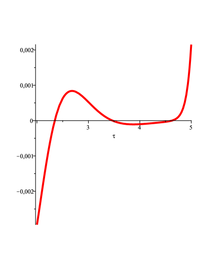
Figure 2: The ODM polynomial $P_{k}(\rho)$ as a function of the scaled variable $\tau=k\rho/A$ for $k=30$. The model problem (31) is being studied.

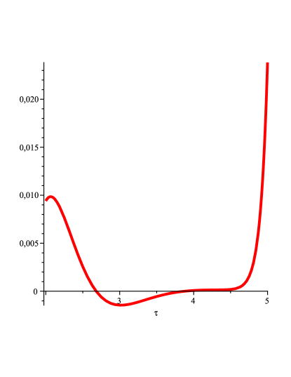
Figure 3: The plot shows $AP^{\prime}_{k}(\rho)/k$ as a function of $\tau=k\rho/A$ for $k=30$, for the model problem (31).

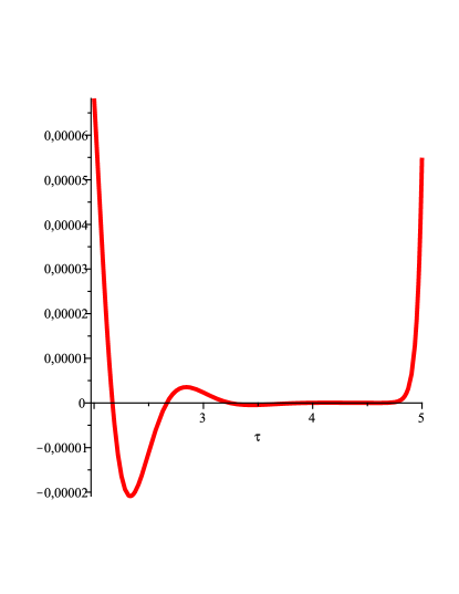
Figure 4: The plot shows $P_{k}(\rho)$ as a function of $\tau=k\rho/A$ for $k=60$, for the model problem (31), demonstrating that a range where $P_{k}(\rho)$ is small persists in higher transformations orders.

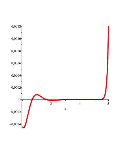
Figure 5: The plot shows $AP^{\prime}_{k}(\rho)/k$ as a function of $\tau=k\rho/A$ for $k=60$, again for the model problem (31). We demonstrate that the favourable region where both $P_{k}(\rho)$ and $P^{\prime}_{k}(\rho)$ are small persists in higher transformations orders.

Figures 2, 3, 4 and 5 show that for $P_{k}(\rho)$, in a rescaled variable $\tau=k\rho/A$, there is an essentially $k$-independent range where $P_{k}(\rho)$ and $P^{\prime}_{k}(\rho)$ are small. This is also the region in the neighbourhood of which the zeros of $P_{k}$ and $P^{\prime}_{k}$ are located. Quite generally, we choose for $\rho_{k}$ the complex zeros of $P^{\prime}_{k}(\rho)$ with the largest real part in this range because they are easy to systematically identify.

The expected theoretical value, obtained by expressing that the real negative and the two complex conjugate solutions of the saddle point equation (23),

$$\lambda= \;-0.1897168\ldots\,,$$ (47a)

$$\lambda= \;0.8448584\ldots\pm\mathrm{i}\,1.386261\ldots\,,$$ (47b)

yield contributions that have the same modulus (which allows for compensation) is $\mu=R/A\approx 4.62987613\ldots$ and then the rate of convergence is predicted to be of the form $0.775^{k}$ from the corresponding estimate (22).

The numerical investigation for $g\to\infty$ extrapolated to $k=\infty$ leads to (see Table 2 and Fig. 6)

$$\lim_{k\to\infty}k\,\mathrm{Re}(\rho_{k})/A=4.65\pm 0.03\,,$$ (48)

yielding a value of $\mu$ significantly smaller than the value $5.31\ldots$ of Table 1 in section III.2 and consistent with the theoretical expectation.

To calculate the ODM approximants, we fit $\rho_{k}$ combining the theoretical asymptotic form and the calculated values of $\rho_{k}$ in the range $k\leq 60$. This is achieved by adding a slightly ad hoc small correction term to the asymptotic formula.

For $g\to\infty$, we define the following quantity which estimates how well the asymptotic strong-coupling limit is approximated by the ODM approximants of order $k$,

$$\delta_{k}=\left|\frac{\left.\mathrm{Re}(Z(g))\,g^{1/6}\right|_{\rm ODM,k}}{\left.Z(g)\,g^{1/6}\right|_{\rm exact}}-1\right|\,.$$ (49)

Some data are then displayed in Table 2 and Fig. 7. From a fit to the numerical data in Fig. 7, One infers a geometric convergence of the form $(0.78\pm 0.02)^{k}$ quite consistent with the theoretical prediction. When $g$ is finite and for $k\to\infty$, the additional factor coming from $\lambda^{k}$ has the form (see Sec. III.2)

$$\lambda^{k}\sim\exp\left(-\frac{k^{3/5}R^{2/5}}{g^{2/5}}\right).$$ (50)

This factor can never cancel the geometric convergence factor and, thus, the ODM approximants converge on the whole Riemann surface.

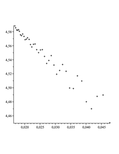
Figure 6: $k\,\mathrm{Re}(\rho_{k})/A$, odd-even averaged, as a function of $1/k$, for the model problem (31). The plot illustrates how the asymptotic limit given in Eq. (48) is approached for $k\to\infty$.

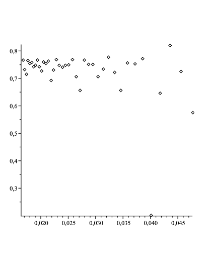
Figure 7: The plot shows $(\delta_{k}/\delta_{19})^{1/(k-19)}$ as a function of $1/k$. We illustrate the asymptotic rate of convergence of the ODM approximants to the strong-coupling limit for the model problem (31), in higher transformation orders beyond $k=19$.

V Quantum mechanics

V.1 Strong coupling limit of the cubic potential

We now consider the spectrum of the Hamiltonian (1), which can be obtained by solving the time-independent Schrödinger equation

$$-\tfrac{1}{2}\psi^{\prime\prime}(x)+\left(\tfrac{1}{2}x^{2}+\tfrac{\mathrm{i}}{6}\,\sqrt{g}\;x^{3}\right)\psi(x)=E\,\psi(x)$$ (51)

with appropriate boundary conditions. The path integral representation of the corresponding partition function has a structure that bears some analogy with the integral (31) discussed in Sec. IV.

The spectrum has an expansion in integer powers of $g$ with real coefficients. For example, for the ground state

$$E_{0}(g)=\frac{1}{2}+\frac{11}{216}\,g-\frac{155}{384}\,g^{2}+\mathcal{O}(g^{3}).$$ (52)

Instanton calculus, based on a steepest descent evaluation of the corresponding path integral, allows us to calculate the classical action relevant for the large order behaviour (3). One finds

$$A=\frac{24}{5}\,.$$ (53)

For $g$ large, from the scaling properties of Eq. (51), one infers that the ground state energy $E_{0}=E_{0}(g)$, as a function of $g$, for large $g$, has an expansion of the form

$$E_{0}=g^{1/5}\sum_{\ell=0}^{\infty}\epsilon_{\ell}\,g^{-2\ell/5}.$$ (54)

This suggests the mapping (see the Appendix)

$$g=\rho\frac{\lambda}{(1-\lambda)^{5/2}}\,,\quad E_{0}=(1-\lambda)^{-1/2}\phi(\lambda,\rho)\,.$$ (55)

In what follows, we again first concentrate on the behaviour of $E_{0}(g)$ for $g\to\infty$, which is related to $\phi(1,\rho)$. More precisely, taking the strong coupling limit $\lambda\to 1$, one finds

$$\phi(1,\rho)=\rho^{1/5}\epsilon_{0}\,.$$ (56)

We now proceed as for the model problem discussed in Sec. IV. Figures 8 and 9 show in a rescaled variable, that there is a range, which is $k$-independent up to corrections of order $k^{-2/5}$, where $P_{k}(\rho)$ and its derivative are small. This is also the region in the neighbourhood of which the zeros of $P_{k}$ and $P^{\prime}_{k}$ are located. We have first determined the complex zeros $\rho_{k}$ of $P^{\prime}_{k}(\rho)$ with the largest real part in this range. Again, these zeros have been chosen because it is easy to identify them systematically.

A fit of the numerical data for orders $k\leq 55$ and an extrapolation to $k\to\infty$ then yields

$$\frac{k\mathrm{Re}(\rho_{k})}{A}=5.5\pm 0.2-\frac{6.0\pm 0.5}{k^{2/5}}\,,$$ (57)

and thus

$$\mu=\frac{R}{A}=5.5\pm 0.2\,,$$ (58)

to be compared with the expected maximum value $\mu=4.895\ldots$ of Table 1.

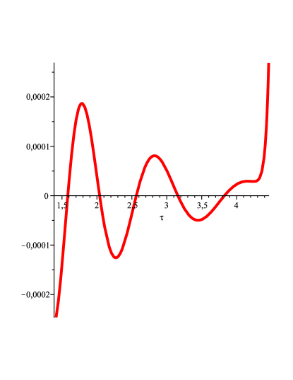
Figure 8: We show $P_{k}(\rho)$ as a function of $\tau=k\rho/A$ for the ODM approximant of order $k=55$ to the ground state energy of the cubic Hamiltonian (51).

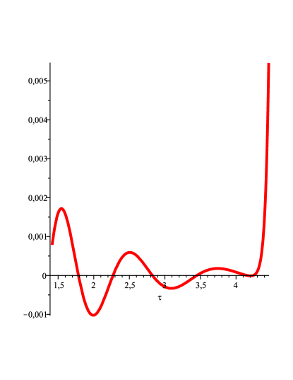
Figure 9: The plot displays $AP^{\prime}_{k}(\rho)/k$ as a function of the scaled variable $\tau=k\rho/A$ for the ODM approximant of transformation order $k=55$ to the ground state energy of the cubic Hamiltonian (51).

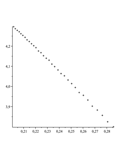
Figure 10: $k\mathrm{Re}(\rho_{k})/A$ as a function of $1/k^{2/5}$. The range for the abscissa is the interval $(0.20,0.29)$, and an extrapolation of the data to $k\to\infty$ is compatible with Eq. (57).

Figure 11: $E_{0,k}$, even-odd averaged, as a function of $1/k^{2/5}$. As $k\to\infty$, the energy converges—under oscillations—to the point indicated as $1/k^{2/5}\to 0$. The plot illustrates the findings of Eqs. (61) and (62).

The numerical relative rate of convergence is compatible with an exponential of the form $0.05\times 0.94^{k}$ and yields the estimate

$$\frac{E_{0}}{g^{1/5}}\mathop{\rightarrow}_{g\to\infty}0.3727\pm 0.0003\,.$$ (59)

However, the value of $\mu$ would lead eventually to a divergence of order $1.2^{k}$. This indicates that the form (57) cannot be used asymptotically. If we take into account the expected value $\mu=4.895\ldots$ and again fit $\mathrm{Re}(\rho_{k})$, we find

$$\frac{k\rho_{k}}{A}=4.895690188-\frac{3.02}{k^{2/5}}\,,$$ (60)

a form we use in the remaining calculations. With this form, we indeed find a smoother convergence with

$$\frac{E_{0}}{g^{1/5}}\mathop{\rightarrow}_{g\to\infty}0.37255\pm 0.00004\,,$$ (61)

at order $55$ to be compared with the value obtained by solving the Schrödinger equation $E_{0}=0.372545791$ rUJJZJxiii .

The errors can be fitted by the form

$$\tfrac{1}{2}(E_{0,k}+E_{0,k-1})=E_{0\,{\rm as.}}$$ (62)

$$-0.00092\,\exp[-0.292\,k^{3/5}]\cos(4.02\,(k^{3/5}-1.20)),$$

where the odd-even averaging improves the fit of the error (and slightly the convergence) by cancelling some subleading oscillatory correction. The form of the oscillatory factor in (62) is just a simple guess (see Fig. 11).

V.2 Finite value of the coupling parameter

For $g$ finite, the additional factor (27) governing the convergence of the ODM approximants in transformation order $k$ is

$$\lambda^{k}\sim\exp\left(-\frac{R^{2/5}\,k^{3/5}}{g^{2/5}}\right)$$ (63)

with

$$R^{2/5}\approx 3.535\ldots\,.$$ (64)

As a check, we have summed the series for $g=5$. The result is

$$E_{0}(5)=0.60168393320519(6),$$ (65)

and the convergence rate of the order of $\mathrm{e}^{-2.10\,k^{3/5}}$. Comparing with the convergence for $g\to\infty$, one finds a variation of the coefficient of $k^{3/5}$ of $1.81$ to be compared with $3.5/g^{2/5}=1.86$.

For $g=1$, the result obtained from a numerical solution of the Schrödinger equation yields

$$E_{0}(1)=0.53078175930417667113556\,,$$ (66)

with all digits being significant. The ODM at order 55 yields (we give its explicit numerical value for illustration)

$$E_{0}(1)=0.53078175930417667113565\,.$$ (67)

The analysis of the convergence is consistent with the theoretical form with a coefficient of $k^{3/5}$ equal to $3.85$ compared to the theoretical expectation of $3.82$.

Finally, to compare with the Padé summation of Ref. rBeWe , we give results for $g=288/49$, which corresponds to $\lambda^{2}=1/7$ in Ref. rBeWe ,

$$k=54\,,\quad E_{0}(\tfrac{288}{49})= \;0.6127381063888\,,$$

$$\Delta E_{0}(\tfrac{288}{49})= \;5.524167213054\,,$$ (68)

$$k=55\,,\quad E_{0}(\tfrac{288}{49})= \;0.6127381063891\,$$

$$\Delta E_{0}(\tfrac{288}{49})= \;5.524167213068\,.$$ (69)

where $\Delta E_{0}=49\,(E_{0}-\tfrac{1}{2})$. At order 54, in Ref. rBeWe one finds $\Delta E_{0}=5.5241683$ and, at order 192, $\Delta E_{0}=5.52416721306031$. The theoretical formula for the ODM methods predicts an error for $\Delta E$ of the order of a few times $10^{-22}$ for $k=192$, confirming the improved convergence achievable by use of the ODM. For completeness, we have verified that $\Delta E_{0}=5.5241672130602221133\dots$ by numerical solution of the Schrödinger equation.

V.3 The imaginary part on the real negative axis

The ODM method converges on the real negative axis and thus the Stieltjes property rVGMMAM , that is, the positivity of the discontinuity, can be verified. For $g\to 0_{-}$ with $\mathrm{Im}(g)>0$, the imaginary part is known analytically from semi-classical considerations (instantons) rUJJZJxiii :

$$\mathrm{Im}E_{0}(g)\mathop{=}_{g\to 0_{-}}\frac{6}{\sqrt{\pi}}\frac{\mathrm{e}^{24/5g}}{\sqrt{-g}}\,\left(1+\frac{169}{576}\,g+\mathcal{O}(g^{2})\right)\,,$$ (70)

where we recall that we are using the cubic Hamiltonian here in the convention (1). For $|g|\to\infty$ and $\mathrm{Im}(g)=0_{+}$, one finds

$$E_{0}(g\to-\infty+\mathrm{i}\,0)\sim(0.301396+\mathrm{i}\,0.218977)\,|g|^{1/5}\,.$$ (71)

Above the negative real axis, the antiresonance energy has a positive imaginary part. For $g=-21.6$, at order 55 we find $E_{0}=0.5540544+0.351399\mathrm{i}$ to be compared with the value $E_{0}=0.554053519+0.351401778\mathrm{i}$ given in rUJJZJxiii . Similarly, for $g=-5+\mathrm{i}0$, $E_{0}=0.4338906+0.1838582\mathrm{i}$, for $g=-1+\mathrm{i}0$, $E_{0}=0.4425200442+0.015517927\mathrm{i}$. In fact, the imaginary part is a simple positive decreasing function providing a smooth interpolation between the two asymptotic forms (see Fig. 12).

Figure 12: The function $-\ln\bigl{(}\mathrm{Im}E_{0}(g)\bigr{)}$ as a function of $-g$.

V.4 Convergence and singularities

Combining Eqs. (62) and (63), one finds that the convergence domain is given by

$$\mathrm{Re}(g^{-2/5})>-0.0826\,.$$ (72)

This contains the sector $|{\rm arg}\,g|<5\pi/4$, that is, the whole Riemann sheet and a sector of the second sheet. Moreover, in the neighbourhood of $g=\infty$, one finds the additional domain

$$|g|>510.0\;[-\cos(2{\rm arg}\,g/5)]^{5/2}.$$ (73)

In the union of these two domains, the function $E_{0}(g)$ is analytic and thus free of level-crossing singularities. In particular, the expansion (54) has about $0.0826$ as a radius of convergence.

VI Conclusions

In this article, we have explored the properties of the order-dependent mapping (ODM) for the summation of the divergent series originating from non-Hermitian Hamiltonians. In these cases, the resulting resonance energies may be complex, and their behaviour may be studied as a function of the complex coupling parameter $g$. In Sec. II, we discuss the motivation for the current study and the two physical problems treated here, which are the cubic anharmonic oscillator in quantum mechanics, and a model problem that counts the number of Feynman diagrams that occur in the perturbative expansion of the partition function of the cubic anharmonic oscillator.

In Sec. III, we recall some important properties of the ODM summation method, and in particular, we describe how the saddle-point approximation helps in determining asymptotic estimates for the parameter $\rho_{k}$ that are needed in order to construct the ODM in higher orders, for the convergence rate of the resulting approximants in the strong coupling limit, and for the analyticity domains of the approximants as the complex phase of the coupling parameter is varied.

In Sec. IV, we discuss the model problem defined in Eq. (IV) which is a simple integral that counts Feynman diagrams in a cubic theory and gives rise to a divergent series. We demonstrate that good approximations to the strong coupling limit can be obtained on the basis of few perturbative terms [see Eq. (46)]. In Sec. V, the analysis is first carried over to the $\mathcal{PT}\,$symmetric cubic potential, with similarly encouraging numerical results, before demonstrating the applicability of the method to manifestly complex resonance energies (see Sec. V.3).

The basic idea of the ODM is that one pretends that the divergent input series, which is to be summed, is in fact a convergent series, but with a circle of convergence whose radius gradually vanishes as the order of the perturbative expansion is increased. This algorithm, together with the representation of the coupling parameter $g$ given in Eq. (6), leads to a very rapid convergence rate of the ODM transforms, in part because the double expansion in $\rho$ and $\lambda$ implied by Eq. (6) represents $g$ as a function of two variables $\rho$ and $\lambda$ whose modulus is bounded by unity for approximants constructed in the strong coupling limit. If one additionally makes a suitable change of variable (and function), in order to incorporate the information about the strong coupling asymptotic expansion (see the Appendix), then one may approximate the strong coupling behaviour using only very few perturbative input data.

Appendix A Parameters in the ODM

Let the strong-coupling asymptotic expansion for the quantity $E(g)$ be known,

$$E(g)=g^{\beta}\sum_{n=0}\epsilon_{n}g^{-n/\alpha}\,,\qquad g\to\infty\,,$$ (74)

a property shared by the two examples we have discussed here (Eqs. (35),(54)) but also by the quartic anharmonic oscillator rsezzin and all $x^{N}$ perturbations to the quantum harmonic oscillator. We consider the conformal mapping $g=\rho\lambda\,(1-\lambda)^{-\alpha}$. This transformation maps the real positive $g$-axis onto the finite $\lambda$ interval $[0,1]$.

For $g\to\infty$, $\lambda\to 1$ and $g$ has an expansion at $\lambda=1$ of the form

$$g^{-1/\alpha}=\sum_{n=0}\Lambda_{n}(1-\lambda)^{n+1}$$ (75)

with $\Lambda_{0}=\rho^{-1/\alpha}$. The function

$$\phi(\lambda)=(1-\lambda)^{\alpha\beta}E\bigl{(}g(\lambda)\bigr{)}$$ (76)

has then a Taylor series expansion at $\lambda=0$,

$$\phi(\lambda)=\sum_{n=0}\phi_{n}\lambda^{n},$$ (77)

as well as at $\lambda=1$,

$$\phi(\lambda)=\sum_{n=0}\varphi_{n}(1-\lambda)^{n}$$ (78)

with $\varphi_{0}=\epsilon_{0}\rho^{\beta}$, where $\epsilon_{0}$ is the coefficient defined in (74). This last property explains, to a large extent, the good convergence of the method even for $g\to\infty$.

References

- (1) R. Seznec, J. Zinn-Justin, Summation of divergent series by order dependent mappings: Application to the anharmonic oscillator and critical exponents in field theory , J. Math. Phys. 20 (1979) 1398–1408.
- (2) J. Zinn-Justin, Summation of divergent series: Order-dependent mapping, arXiv:1001.0675 [math-ph].
- (3) J. C. Le Guillou and J. Zinn-Justin, The hydrogen atom in strong magnetic fields: summation of the weak field series expansion, Ann. Phys. (N.Y.) 147 (1983), 57-84.
- (4) R. Guida and J. Zinn-Justin, 3D Ising model: the scaling equation of state, Nucl. Phys. B489 (1997) 626-652.
- (5) J. L. Kneur, M.B. Pinto, R.O. Ramos, Asymptotically improved convergence of optimized perturbation theory in the Bose-Einstein condensation problem, Phys. Rev. A 68 (2003) 043615.
- (6) J. L. Kneur, M. B. Pinto, R. O. Ramos, Critical and tricritical points for the massless 2D Gross–Neveu model beyond large , Phys. Rev. D 74 (2006) 125020.
- (7) J. L. Kneur, M. B. Pinto, R. O. Ramos, E. Staudt, Emergence of tricritical point and liquid-gas phase in the massless 2+1 dimensional Gross–Neveu model, Phys. Rev. D 76 (2007) 045020.
- (8) A. Duncan, H. F. Jones, Convergence proof for optimized expansion: Anharmonic oscillator, Phys. Rev. D 47 (1993) 2560-2572.
- (9) R. Guida, K. Konishi, H. Suzuki, Improved Convergence Proof of the Delta Expansion and Order Dependent Mappings, Ann. Phys. 249 (1996) 109-145.
- (10) W. E. Caswell, Accurate energy levels for the anharmonic oscillator and a summable series for the double-well potential in perturbation theory, Ann. Phys. 123 (1979) 153-184.
- (11) P. Dorey, C. Dunning and R. Tateo, Spectral equivalences, Bethe ansatz equations, and reality properties in PT-symmetric quantum mechanics, J. Phys. A 34 (2001) L391; ibid. 34 (2001) 5679-5704.
- (12) K. C. Shin, On the reality of eigenvalues for a class of PT-symmetric oscillators, Commun. Math. Phys. 229 (2002) 543-564.
- (13) M. E. Fisher, Yang–Lee Edge Singularity and Field Theory, Phys. Rev. Lett. 40 (1978) 1610-1613.
- (14) C. M. Bender, D. C. Brody and H. F. Jones, Scalar Quantum Field Theory with Cubic Interaction, Phys. Rev. Lett. 93 (2004) 251601.
- (15) L. N. Lipatov, Divergence of the perturbation-theory series and pseudoparticles, JETP Lett. 25 (1977) 104-107; Divergence of the perturbation-theory series and the quasi-classical theory, Sov. Phys. JETP 45 (1977) 216-223.
- (16) E. Brézin, J. C. Le Guillou, J. Zinn-Justin, Perturbation theory at large order. I. The interaction, Phys. Rev. D 15 (1977) 1544-1557.
- (17) J. Zinn-Justin, Perturbation series at large orders in quantum mechanics and field theories: application to the problem of resummation, Phys. Rep. 70 (1981) 109–167.
- (18) E. Caliceti, S. Graffi, and M. Maioli, Perturbation theory of odd anharmonic oscillators, Comm. Math. Phys. 75 (1980) 51-66.
- (19) C. M. Bender and S. Boettcher, Real spectra in non-hermitian Hamiltonian having PT symmetry, Phys. Rev. Lett. 80 (1998) 5243.
- (20) C. M. Bender, D. C. Brody, and H. F. Jones, Complex Extension of Quantum Mechanics, Phys. Rev. Lett. 89, 270402 (2002) and Am. J. Phys. 71, 1095 (2003).
- (21) C. M. Bender, Making sense of non-Hermitian Hamiltonians, Rep. Prog. Phys. 70 (2007) 947-1018.
- (22) V. Grecchi, M. Maioli and A. Martinez, Pad summability of the cubic oscillator, J. Phys. A: Math. Theor. 42 (2009) 425208.
- (23) C. M. Bender, E. J. Weniger, Numerical evidence that the perturbation expansion for a non-Hermitian PT-symmetric Hamiltonian is Stieltjes, J. Math. Phys. 42 (2001) 2167-2183.
- (24) E. Caliceti, Distributional Borel summability of odd anharmonic oscillators, J. Phys. A 33 (2000) 3753-3770.
- (25) H. Kleinert, W. Janke, Convergence behavior of variational perturbation expansion — A method for locating Bender-Wu singularities, Phys. Lett. A 206 (1995) 283-289.
- (26) U. D. Jentschura, A. Surzhykov, J. Zinn-Justin, Generalized nonanalytic expansions, PT-symmetry and large order formulas for odd anharmonic oscillators, SIGMA 5 (2009) 005.
- (27) U. D. Jentschura, J. Zinn-Justin, Calculation of the Characteristic Functions of Anharmonic Oscillators, ArXiv:1001.4313 [math-ph].