Condensate entanglement and multigap superconductivity in nanoscale superconductors

Abstract

A Green functions approach is used to study superconductivity in nanofilms and nanowires. We show that the superconducting condensate results from the multimodal entanglement, or internal Josephson coupling, of the subcondensates associated with the manifold of Fermi surface subparts resulting from size-quantisation. This entanglement is of critical importance in these systems, since without it superconductivity would be extremely weak, if not completely negligible. Further, the multimodal character of the condensate generally results in multigap superconductivity, with great quantitative consequence for the value of the critical parameters. Our approach suggests that these are universal characteristics of confined superconductors.

In recent years, superconductivity has been studied with great interest in nanoscale systems, such as nanofilms (NFs) guo04 ; eom06 ; qin09 ; zhang10 and nanowires (NWs) tian05 ; zgirski07 . From the theory point of view, there was interest in superconductivity in NFs blatt63 long before the advent of nanoscience. The great advances in materials synthesis technology, however, allows today the fabrication of high quality nanoscale samples, in which the effects of confinement, or quantum size effects, can be closely examined. Thus, for instance, the oscillations of the superconducting gap with film thickness predicted in Ref. blatt63, have now been observed convincingly in experiment, albeit with a weaker amplitude than the one predicted guo04 ; eom06 ; qin09 . Recent theoretical work has shown similar quantum size-induced oscillations in the critical temperature, specific heat, and critical field in NFs chen06 ; shanenko07 as well as in NWs han04 ; shanenko06 . Interestingly, it is found that, for sufficiently small confinement length (i.e., film thickness or wire radius), the oscillations can drive the critical temperature well above the bulk value. This was not observed in the ultrathin NFs of Refs. guo04, ; eom06, ; qin09, , but appears to be the case in the NFs of Ref. court08, , and also in NWs tian05 ; zgirski07 .

Here we show that confinement has far reaching consequences regarding the character of the superconducting condensate itself. In this regard, the study of superconductivity in nanosystems is of broader interest. Indeed, superfluidity also fascinates researchers in atomic physics schunck08 and nuclear physics pastore08 , where confinement occurs only naturally. Superfluidity is a macroscopic quantum phenomenon, in which the order parameter, or condensate “wave function” plays a central role. Thus, much effort is put in trying to characterise it in the different systems in which superfluidity is observed schunck08 ; fernandes10 . In this work, we use a Green functions approach to superconductivity in nanosystems, bringing to light previously unrecognised but significant confinement effects. We find that the splitting of the Fermi surface in a discrete set of nonintersecting parts because of the size-quantisation of the energy levels results inevitably in a condensate of composite nature. That is, the condensate arises from the multimodal entanglement, or internal Josephson coupling leggett66 ; hines03 , of the subcondensates associated with the Fermi surface subparts. Further, the entanglement is crucial, because without it the systems collapses into uncorrelated subcondensates, in which superconductivity is dramatically weaker, if not completely negligible. Finally, the manifold of subcondensates will generally result in multigap superconductivity, with significant impact on the predicted value of the critical temperature, compared to single-gap models. The generality of our formalism suggests that these characteristics are universal properties of confined superconductors.

Consider a system of quasiparticles with a weak attractive effective interaction coupling only particles with opposite spin (e.g., the net effect of phonon exchange and the screened Coulomb interaction), which will eventually couple only particles near the Fermi level (chemical potential), $\mu$. We have the Hamiltonian $\hat{H}=\hat{H}_{0}+\hat{H}_{I}-\mu\hat{N}$, where $\hat{H}_{0}$ describes the noninteracting system, $\hat{N}$ is the number operator, and $\hat{H}_{I}={1\over 2}\int d^{3}r\,d^{3}r^{\prime}\hat{\psi}_{\uparrow}^{\dagger}({\bf r})\hat{\psi}_{\downarrow}^{\dagger}({\bf r}^{\prime})v_{\rm eff}({\bf r},{\bf r}^{\prime})\hat{\psi}_{\downarrow}^{\dagger}({\bf r}^{\prime})\hat{\psi}_{\uparrow}({\bf r}).$ Consider next the Green function, ${\cal G}({\bf r}{\bf r}^{\prime},\tau)=-\langle T_{\tau}\hat{\psi}_{\uparrow}^{\dagger}({\bf r}\tau)\hat{\psi}_{\uparrow}^{\phantom{\dagger}}({\bf r}^{\prime}0)\rangle$. As in BCS theory fetter71 , to solve the equation of motion for ${\cal G}$ we introduce the Gorkov functions ${\cal F}({\bf r}{\bf r}^{\prime},\tau)=-\langle T_{\tau}\hat{\psi}_{\uparrow}({\bf r}\tau)\hat{\psi}_{\downarrow}({\bf r}^{\prime}0)\rangle$ and ${\cal F}^{\dagger}({\bf r}{\bf r}^{\prime},\tau)=-\langle T_{\tau}\hat{\psi}_{\downarrow}^{\dagger}({\bf r}\tau)\hat{\psi}_{\uparrow}^{\phantom{\dagger}}({\bf r}^{\prime}0)\rangle$, and take the mean-field approximation $\langle T_{\tau}\hat{\psi}_{\downarrow}^{\dagger}({\bf r}_{1}\tau_{1})\hat{\psi}_{\downarrow}^{\phantom{\dagger}}({\bf r}_{2}\tau_{2})\hat{\psi}_{\uparrow}^{\phantom{\dagger}}({\bf r}_{3}\tau_{3})\hat{\psi}_{\uparrow}^{\dagger}({\bf r}_{4}\tau_{4})\rangle\simeq-{\cal F}({\bf r}_{3}{\bf r}_{2},\tau_{3}-\tau_{2}){\cal F}^{\dagger}({\bf r}_{1}{\bf r}_{4},\tau_{1}-\tau_{4})$. The resulting coupled equations for ${\cal G}$ and ${\cal F}^{\dagger}$ read, in frequency domain,

$${\cal L}_{p}({\bf r})\tilde{\cal G}({\bf r}{\bf r}^{\prime},\omega_{p})-\int d^{3}x\Delta({\bf r}{\bf x})\tilde{\cal F}^{\dagger}({\bf x}{\bf r}^{\prime},\omega_{p})=\hbar\delta({\bf r}-{\bf r}^{\prime}),$$

$${\cal L}_{p}({\bf r})\tilde{\cal F}^{\dagger}({\bf r}{\bf r}^{\prime},\omega_{p})-\int d^{3}x\Delta({\bf r}{\bf x})\tilde{\cal G}({\bf x}{\bf r}^{\prime},\omega_{p})=0.$$ (1)

Here, ${\cal L}_{p}({\bf r})=i\hbar\omega_{p}-H_{0}({\bf r})+\mu$, with $\omega_{p}$ is a fermionic frequency, $\tilde{\phantom{G}}$ denoting a $\tau$-Fourier transformed function, and we have introduced $\Delta({\bf r}{\bf r}^{\prime\prime})\equiv v_{\rm eff}({\bf r},{\bf r}^{\prime\prime}){\cal F}({\bf r}{\bf r}^{\prime\prime},0)$, i.e., a nonlocal pairing potential pastore08 ; bruder90 .

Assume now that $H_{0}$ is such that its eigenstates form an orthonormal set, i.e., $H_{0}|\nu\rangle=E_{\nu}|\nu\rangle$, with $\langle\nu|\nu^{\prime}\rangle=\delta_{\nu,\nu^{\prime}}$. Inserting the expansions $\hat{\psi}_{\sigma}({\bf r}\tau)=\sum_{\nu}\psi_{\nu}({\bf r})c_{\nu\sigma}(\tau)$ and $\hat{\psi}^{\dagger}_{\sigma}({\bf r}\tau)=\sum_{\nu}\psi^{*}_{\nu}({\bf r})c^{\dagger}_{\nu\sigma}(\tau)$ in Eqs. (1) leads to [with, e.g., $\tilde{\cal G}({\bf r}{\bf r}^{\prime},\omega_{p})=\sum_{\nu\nu^{\prime}}\psi_{\nu}({\bf r})\psi^{*}_{\nu^{\prime}}({\bf r}^{\prime})\tilde{\cal G}(\nu\nu^{\prime},\omega_{p})$]

$$\left[i\hbar\omega_{p}-\epsilon_{\nu}\right]\tilde{\cal G}(\nu\nu^{\prime},\omega_{p})+\sum_{\kappa}\Delta(\nu\kappa)\tilde{\cal F}^{\dagger}(\kappa\nu^{\prime},\omega_{p})=\hbar\delta_{\nu\nu^{\prime}},$$

$$\left[i\hbar\omega_{p}+\epsilon_{\nu}\right]\tilde{\cal F}^{\dagger}(\nu\nu^{\prime},\omega_{p})+\sum_{\kappa}\Delta^{*}(\nu\kappa)\tilde{\cal G}(\kappa\nu^{\prime},\omega_{p})=0.$$ (2)

Here, $\epsilon_{\nu}=E_{\nu}-\mu$ and $\Delta(\nu\nu^{\prime})=\sum_{\kappa\kappa^{\prime}}V_{\nu\nu^{\prime},\kappa\kappa^{\prime}}{\cal F}(\kappa\kappa^{\prime},0),$ with $V_{\nu\nu^{\prime},\kappa\kappa^{\prime}}\equiv=-\langle\nu\nu^{\prime}|v_{\rm eff}|\kappa\kappa^{\prime}\rangle$. The formal solution of Eqs. (2) can readily be written in closed form. But we further assume that $v_{\rm eff}$ couples only time-reversed states anderson59 . If $|-\!\nu\rangle$ and $|\nu\rangle$ denote time-reversed states, we have $V_{\nu\nu^{\prime},\kappa\kappa^{\prime}}=V_{\nu\,-\!\nu,\kappa\,-\!\kappa}\delta_{-\nu\,\nu^{\prime}}\delta_{-\kappa\,\kappa^{\prime}}\equiv V_{\nu\kappa}\delta_{-\nu\,\nu^{\prime}}\delta_{-\kappa\,\kappa^{\prime}}$ and $\Delta(\nu\nu^{\prime})=\delta_{-\nu\nu^{\prime}}\sum_{\kappa}V_{\nu\kappa}{\cal F}(-\!\kappa\,\kappa,0)\equiv\Delta(\nu)\delta_{-\nu\nu^{\prime}}$. As in BCS theory, it is straightforward to deduce that $\tilde{\cal G}(\nu\nu^{\prime},\omega_{p})=-\delta_{\nu\nu^{\prime}}(i\omega_{p}+\epsilon_{\nu}/\hbar)/(\omega_{p}^{2}+\xi_{\nu}^{2}/\hbar^{2})$ and $\tilde{\cal F}^{\dagger}(\nu\nu^{\prime},\omega_{p})=\delta_{-\nu\nu^{\prime}}(\Delta^{*}(\nu)/\hbar)/(\omega_{p}^{2}+\xi^{2}_{\nu}/\hbar^{2}),$ with $\xi^{2}_{\nu}=\epsilon_{\nu}^{2}+|\Delta(\nu)|^{2}$. Thus, the gap values are given by the coefficients of the expansion of $\Delta({\bf r}{\bf r}^{\prime\prime})$ over the quasiparticle states. Finally, noting that ${\cal F}(-\!\kappa\,\kappa,0)=\sum_{p}\tilde{\cal F}(-\!\kappa\,\kappa,\omega_{p})/\beta\hbar,$ we obtain the gap equation

$$\Delta(\nu)=\sum_{\nu^{\prime}}V_{\nu\nu^{\prime}}\Delta(\nu^{\prime}){1\over{2\xi_{\nu^{\prime}}}}\tanh{{\xi_{\nu^{\prime}}}\over{{2k_{\rm B}T}}}.$$ (3)

Once $\Delta(\nu)$ is determined, the condensate wave function, defined by $\Psi({\bf r}{\bf r}^{\prime})\equiv{\cal F}({\bf r}{\bf r}^{\prime},0)$ leggett08 , and the pairing potential can be calculated from

$$\Psi({\bf r}{\bf r}^{\prime})=\sum_{\nu}\psi_{\nu}({\bf r})\psi_{-\nu}({\bf r}^{\prime})\Delta(\nu){1\over{2\xi_{\nu}}}\tanh{{\xi_{\nu}}\over{2k_{\bf B}T}},$$ (4)

$$\Delta({\bf r}{\bf r}^{\prime})=\sum_{\nu}\psi_{\nu}({\bf r})\psi_{-\nu}({\bf r}^{\prime})\Delta(\nu).$$ (5)

In the following we apply our formalism to NFs and NWs. We take parameters corresponding to Al comment0 , which is a weak coupling superconductor (so a mean-field approach is applicable), and is also free-electron-like. Given that the spatial dependence of $v_{\rm eff}$ is not really known, it is best to use phenomenologically motivated $V_{\nu\nu^{\prime}}$’s in Eq. (3) (thereby, implicitly defining the spatial form of $v_{\rm eff}$). We use as reference the BCS coupling constant for the bulk material, $V_{0}$, estimated from the experimental value of $T_{c}$ and $k_{\rm B}T_{c}=1.13\hbar\omega_{D}e^{-1/N_{0}V_{0}}$ fetter71 . Below, unless otherwise stated, energies are in Rydbergs (Ry), and lengths in $a_{0}$.

To model a NF we follow Ref. thompson63, . Briefly, the system of quasiparticles is in a potential well defined by two large planes of side $L$, a distance $d$ apart, with $V({\bm{\rho}},z)=0$ for $0\leq z\leq d$, and $\infty$ otherwise. The quasiparticles states are $\psi_{{\bf q}n}({\bm{\rho}},z)=(2/L^{2}d)^{1/2}e^{i{\bf q}\cdot{\bm{\rho}}}\sin a_{n}z,$ where $a_{n}=\pi n/d$ and ${\bf q}=2\pi(l,m)/L$, with $l,m\in\mathbb{Z}$. Thus, $|\nu\rangle=|{\bf q}n\rangle$ and $|-\!\nu\rangle=|-\!{\bf q}n\rangle$ are time-reversed states. The energy levels are given by $E_{{\bf q}n}=q^{2}+a_{n}^{2}$ (for simplicity, the quasiparticle mass is taken equal to the bare electron mass). The Fermi “surface” breaks into a set of concentric circumferences of radii $q_{\rm F}^{(n)}=(\mu-a_{n}^{2})^{1/2}.$ For the $V_{\nu\nu^{\prime}}$ in Eq. (3) we take a BCS-type model fetter71 ,

$$V_{{\bf q}n,{\bf q}^{\prime}n^{\prime}}={{U_{nn^{\prime}}}\over{L^{2}d}}\theta(\epsilon_{w}-|\epsilon_{{\bf q}n}|)\theta(\epsilon_{w}-|\epsilon_{{\bf q}^{\prime}n^{\prime}}|),$$ (6)

$\epsilon_{w}$ defining the energy window around $\mu$ within which $v_{\rm eff}$ is effective. We estimate the $U_{nn^{\prime}}$ with a contact potential $v_{\rm eff}({\bf r}-{\bf r}^{\prime})=-V_{0}\delta({\bf r}-{\bf r}^{\prime})$ fetter71 ; comment1 , hence $U_{nn^{\prime}}=V_{0}(1+\delta_{nn^{\prime}}/2)$ thompson63 . Note that Eq. (6) will lead in general to a multigap equation, similar to the expression of Suhl et al. suhl59 . But because the contact interaction results in off-diagonal $U_{nn^{\prime}}$’s that are all equal, there is only one gap. Thereafter, it is straightforward to derive the results of previous authors (cf., e.g., Refs. shanenko07, ; thompson63, ).

It is important to recognise, however, is that even with the simple contact potential, this still is a system with multiple subcondensates. To see this, we rewrite the Hamiltonian in second-quantised form. In close analogy to the two band case studied by Leggett leggett66 , one finds $\hat{H}=\hat{H}_{\rm D}+\hat{H}_{\rm J}$, with

$$\hat{H}_{\rm D}=\sum_{n}\Big{[}\sum_{{\bf q}\sigma}\epsilon_{{\bf q}n\sigma}c^{\dagger}_{{\bf q}n\sigma}c^{\phantom{\dagger}}_{{\bf q}n\sigma}$$

$$\phantom{MMMMMM}-U_{n}\sum_{{\bf q}{\bf q}^{\prime}}c^{\dagger}_{{\bf q}n\uparrow}c^{\dagger}_{-{\bf q}n\downarrow}c^{\phantom{\dagger}}_{-{\bf q}^{\prime}n\downarrow}c^{\phantom{\dagger}}_{{\bf q}^{\prime}n\uparrow}\Big{]}$$

$$\hat{H}_{\rm J}=\sum_{n\neq n^{\prime}}\Big{[}-J\sum_{{\bf q}{\bf q}^{\prime}}c^{\dagger}_{{\bf q}n\uparrow}c^{\dagger}_{-{\bf q}n\downarrow}c^{\phantom{\dagger}}_{-{\bf q}^{\prime}n^{\prime}\downarrow}c^{\phantom{\dagger}}_{{\bf q}^{\prime}n^{\prime}\uparrow}\Big{]}.$$ (7)

Here, $\hat{H}_{\rm D}$ is the Hamiltonian of the independent condensates, with $U_{n}=3V_{0}/2$, while $\hat{H}_{\rm J}$ represents an internal Josephson coupling leggett66 , with $J=V_{0}$.

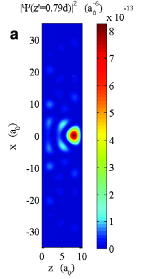
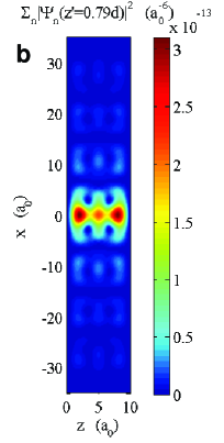
Figure 1: (color online) Condensate probability density (a) $|\sum_{n}\Psi_{n}({\bm{\rho}},z;z^{\prime})|^{2}$ and $\sum_{n}|\Psi_{n}({\bm{\rho}},z;z^{\prime})|^{2}$ (b), plotted in the $xOz$ plane, at $z^{\prime}=0.79d$, for $d=10\,a_{0}$ (see text). In (b) there are no interference effects.

Thus, the condensate is given by a multimodal entanglement of subcondensates hines03 . The entanglement is beautifully illustrated by the resulting interference pattern in the probability density, $|\Psi({\bf r}{\bf r}^{\prime})|^{2}$. In the present case, Eq. (4) leads to $\Psi=\Psi({\bm{\rho}},z;z^{\prime})=\sum_{n}\Psi_{n}({\bm{\rho}},z;z^{\prime})$, with (at $T=0$ K)

$$\Psi_{n}({\bm{\rho}},z;z^{\prime})={\Delta\over{4\pi^{2}d}}I_{n}({\bm{\rho}})\sin a_{n}z\sin a_{n}z^{\prime},$$ (8)

where $I_{n}({\bm{\rho}})=\int^{\prime}dq\,qJ_{0}(q|{\bm{\rho}}|)/\xi_{{\bf q}n}$ comment2 . Given two quasiparticles of opposite spin, at $(0,z^{\prime})$ and $({\bm{\rho}},z)$, respectively, $\Psi({\bm{\rho}},z;z^{\prime})$ is their pairing probability amplitude. In Fig. 1(a), we plot $|\sum_{n}\Psi_{n}({\bm{\rho}},z;z^{\prime})|^{2}$ for $({\bm{\rho}},z)$ in the $xOy$ plane, for a $d=10\,a_{0}$ NF, and contrast it to $\sum_{n}|\Psi_{n}({\bm{\rho}},z;z^{\prime})|^{2}$ [cf. Fig. 1(b)], to highlight the interference effects. To choose $z^{\prime}$, we calculated first the local pair density, $\varrho_{s}(z^{\prime})\equiv\int d^{2}\rho\,dz|\Psi({\bm{\rho}},z;z^{\prime})|^{2}$. One readily finds $\varrho_{s}(z^{\prime})=(\Delta/16\pi^{3}d)\arctan(\epsilon_{w}/\Delta)\sum_{n}\sin^{2}a_{n}z^{\prime}$. In Fig. 2(a) we plot $\varrho_{s}(z^{\prime})$ for three $d$ values. For $d=10\,a_{0}$, $\varrho_{s}(z^{\prime})$ is maximum at $z^{\prime}=0.79d$ (note that the number of maxima in $\varrho_{s}(z^{\prime})$ corresponds the number of subcondensates in the film).

Furthermore, the strength of the $J$ coupling is of critical importance, its magnitude largely determining the value of the critical parameters. Indeed, for a renormalised coupling $J=fV_{0}$, with $f\leq 1$, both $\Delta$ and $T_{c}$ fall dramatically as $f$ decreases. We illustrate this in Fig. 2(b), for $d=10$ $a_{0}$. At $f=1$, the critical parameters are significantly higher than the bulk values, namely $T_{c}/T_{c}^{b}=2.51$ and $\Delta/\Delta^{b}=2.60$. For $f=0$, i.e., decoupled condensates, $\Delta/\Delta^{b}$ and $T_{c}/T_{c}^{b}$ are negligible, of the order of $10^{-3}.$ In contrast, in Refs. guo04, ; eom06, ; qin09, , $\Delta$ and $T_{c}$ are found to be a large fraction of the bulk values, requiring $0.5\lesssim f<1$ in our model, i.e., a substantial coupling. A value $f<1$ is easily understood, since interband pair scattering requires a minimum momentum transfer, so has a smaller scattering phase space volume than intraband scattering [an aspect not accounted for in Eq. (6)]. In fact, this may be another reason why in experiment the critical parameters are lower than in the bulk.

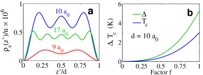
Figure 2: (color online) (a) Local pair density, $\varrho_{s}(z^{\prime})$, for three $d$ values (in units of the bulk electron density, $n$). The number of maxima indicate the number of subcondensates. (b) $\Delta$ and $T_{c}$ change strongly with factor $f$ (see text). At $f=0$ (decoupled condensates), $T_{c}\simeq 10^{-3}T_{c}^{b}$, and $\Delta\simeq 10^{-3}\Delta^{b}$.

We now turn our attention to NWs. The quasiparticles are now in a cylindrical potential well of radius $R$ and length $L$: $V(\rho,\phi,z)=0$ for $\rho\leq R$, and $\infty$ otherwise. The quasiparticle states are han04 $\psi_{kmn}(\rho,\phi,z)=[\pi R^{2}LJ_{|m|+1}^{2}(\eta_{mn})]^{-1/2}J_{|m|}(\rho\eta_{mn}/R)e^{i(kz+m\phi)},$ where $J_{m}$ is the $m$-th order Bessel function of the 1st kind and $\eta_{mn}$ is its $n$-th zero abramowitz72 , and $k=2\pi l/L$, with $l\in\mathbb{Z}$. Here, $|\nu\rangle=|kmn\rangle$ and $|-\!\!\nu\rangle=|-\!\!k\,-\!\!m\,n\rangle$ are time-reversed states. The eigenenergies are given by $E_{kmn}=k^{2}+\eta_{mn}^{2}/R^{2}$, and the Fermi surface reduces to a discrete set $\{-k_{\rm F}^{(mn)},k_{\rm F}^{(mn)}\}^{\phantom{\dagger}}_{mn}$. The energy bands are now 1-dimensional, while they were 2-dimensional in the NFs. This gives rise to important quantitative differences between the two cases regarding the behaviour of their properties as a function of confining length han04 ; shanenko06 . Here we focus, however, on the multigap character of superconductivity in NWs. To see this, let us approximate the $V_{\nu\nu^{\prime}}$ in Eq. (3) by

$$V_{kmn,k^{\prime}m^{\prime}n^{\prime}}={U_{mn,m^{\prime}n^{\prime}}\over{\pi^{2}RL}}\theta(\epsilon_{w}-|\epsilon_{kmn}|)\theta(\epsilon_{w}-|\epsilon_{k^{\prime}m^{\prime}n^{\prime}}|).$$ (9)

To estimate the $U_{mn,m^{\prime}n^{\prime}}$ we again use a contact potential. Unlike the NF case, the off-diagonal elements are different from each other. This immediately results in multiple gaps, $\Delta_{mn}$. In Fig. 3(a) we plot the gap values as a function of temperature for a $R=7.5\,a_{0}$ NW comment5 . In this case there are seven occupied bands, thus seven subcondensates. The $\Delta_{mn}(0)$ values depend on the interplay between the $U_{mn,m^{\prime}n^{\prime}}$ strengths and how far from $\mu$ are the bottoms of the bands [recall that in 1-dimension the density of states has an (integrable) singularity at $k=0$].

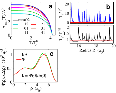
Figure 3: (color online) (a) Plot of the seven $\Delta_{mn}(T)$ in a $R=7.5\,a_{0}$ NW; $T_{c}=4.2\,T_{c}^{b}$. (b) Upper panel: $T_{c}$ as a function of $R$. $T_{c}$ increases sharply when a new band starts to be occupied. The horizontal line indicates $T_{c}^{b}$. For large $R$, $T_{c}$ tends to $T_{c}^{b}$ (not shown here). Lower panel: The ratio of $T_{c}$ to the single-gap value, $T_{c}^{sg}$, shows that they differ significantly. (c) The pairing potential, $\Delta$, and order parameter, $\Psi$, are not proportional to each other (here shown in the ${\bf r}={\bf r}^{\prime}$ limit).

$T_{c}$ and the $\Delta_{mn}$ oscillate strongly as a function $R$, rising sharply when the bottom of a newly occupied band falls below $\mu$ as $R$ increases. This is illustrated for $T_{c}$ in Fig. 3(b) (upper panel) comment6 . Although similar to the oscillations found in single-gap models han04 ; shanenko06 , the multigap character of the condensate results in significant quantitative differences. Indeed, Fig. 3(b), lower panel, shows the plot of the ratio of $T_{c}$’s obtained in the multigap and single-gap cases (the latter, $T_{c}^{sg}$, is obtained by approximating the $U_{mn,m^{\prime}n^{\prime}}$ by their average value, $\bar{U}_{mn,m^{\prime}n^{\prime}}$). We see that $T_{c}^{sg}$ can be more than 100% too low respect to the multigap value. As one would expect, the magnitude of the $J$ coupling is just as critical here as in NFs. Indeed, setting $U_{mn\neq m^{\prime}n^{\prime}}=0$ in the gap equation results in uncorrelated condensates, with $T_{c}^{(mn)}$ values largely reduced respect to the true $T_{c}$. For example, in a $R=5$ $a_{0}$ NW, for which $T_{c}=2.12\,T_{c}^{b}$, there would be three condensates, with critical temperatures $T_{c}^{(21)}\simeq 0.078\,T_{c}^{b}$, $T_{c}^{(11)}\simeq 10^{-5}\,T_{c}^{b}$, and $T_{c}^{(01)}\simeq 10^{-12}\,T_{c}^{b}$.

We add that, because the matrix elements decrease with confining length, a finite $J$ coupling is essential to obtain the bulk values of the critical parameters in the limit of large systems (i.e., $R\to\infty$ in NWs and $d\to\infty$ in NFs). Also, as defined in Eqs. (4) and (5), the pairing potential and the order parameter are not proportional to each other (unlike in homogeneous systems fetter71 ), even in the ${\bf r}={\bf r}^{\prime}$ limit. For example, in Fig. 3(c) we compare $\Delta(\rho)$ (renormalised, for comparison) and $\Psi(\rho)$ (in that limit both depend only on $\rho$) for the $R=7.5\,a_{0}$ wire. So our $\Delta(\rho)$ is not equivalent to the “order parameter” in other approaches han04 ; shanenko06 . Also, our $\Delta(\rho)$ should not be confused with the spatially varying gap seen, e.g., in some high-$T_{c}$ superconductors mcelroy05 . Indeed, in our case the gap(s) are constant throughout the system.

We thank J. Tempere for fruitful discussions. This work was supported by FWO-Vl and the Belgian Science Policy (IAP).

References

• (1) Y. Guo, Y.-F. Zhang, X.-Y. Bao, T.-Z. Han, Zhe Tang, L.-X. Zhang, W.-G. Zhu, E. G. Wang, Q. Niu, Z. Q. Qiu, J.-F. Jia, Z.-X. Zhao, and Q.-K. Xue, Science 306, 1915 (2004).
• (2) D. Eom, S. Qin, M.-Y. Chou, and C. K. Shih, Phys. Rev. Lett. 96, 027005 (2006).
• (3) S. Qin, J. Kim, Q. Niu, and C.-K. Shih, Science 324, 1314 (2009).
• (4) T. Zhang, P. Cheng, W.-J. Li, Y.-J. Sun, G. Wang, X.-G. Zhu, K. He, L. Wang, X. Ma, X. Chen, Y. Wang, Y. Liu, H.-Q. Lin, J.-F. Jia, and Q.-K. Xue, Nature Phys. 6 104, (2010).
• (5) M. Tian, J. Wang, J. S. Kurtz, Y. Liu, M. H. W. Chan, T. S. Mayer, and T. E. Mallouk, Phys. Rev. B 71, 104521 (2005).
• (6) M. Zgirski and K. Y. Arutyunov, Phys. Rev. B 75, 172509 (2007).
• (7) J. M. Blatt and C. J. Thompson, Phys. Rev. Lett. 10, 332 (1963).
• (8) B. Chen, Z. Zhu, and X. C. Xie, Phys. Rev. B 74, 132504 (2006).
• (9) A. A. Shanenko, M. D. Croitoru, and F. M. Peeters, Phys. Rev. B 75, 014519 (2007).
• (10) J. E. Han and V. H. Crespi, Phys. Rev. B 69, 214526 (2004).
• (11) A. A. Shanenko and M. D. Croitoru, Phys. Rev. B 73, 012510 (2006).
• (12) N. A. Court, A. J. Ferguson, and R. G. Clark, Supercond. Sci. Technol. 21, 015013 (2008).
• (13) C. H. Schunck, Y. Shin, A. Schirotzek, and W. Ketterle, Nature (London) 454, 739 (2008).
• (14) A. Pastore, F. Barranco, R. A. Broglia, and E. Vigezzi, Phys. Rev. C 78, 024315 (2008).
• (15) R. M. Fernandes, D. K. Pratt, W. Tian, J. Zarestky, A. Kreyssig, S. Nandi, M. G. Kim, A. Thaler, N. Ni, P. C. Canfield, R. J. McQueeney, J. Schmalian, and A. I. Goldman, Phys . Rev. B 81 140501(R), 2010.
• (16) A. J. Leggett, Prog. Theor. Phys. 36, 901 (1966).
• (17) A. P. Hines, R. H. McKenzie, and G. J. Milburn, Phys. Rev. A 67, 013609 (2003).
• (18) A. L. Fetter and J. D. Walecka, Quantum Theory of Many-Particle systems, (McGraw-Hill, New York, 1971).
• (19) Chr. Bruder, Phys. Rev. B 41, 4017 (1990).
• (20) P. W. Anderson, J. Phys. Chem. Solids 11, 26 (1959).
• (21) A. J. Leggett, in Superconductivity, Vol. 1, edited by K. H. Bennemann and J. B. Ketterson (Springer-Verlag, Berlin, 2008).
• (22) The particle density is $r_{s}=2.07\,a_{0}$, the (bulk) critical parameters are $T_{c}^{b}=1.2$ K and $\Delta^{b}=1.7k_{B}T_{c}^{b}$, and density of states per spin ($N_{0}$) is obtained with the electron gas expression ashcroft76 ; $\hbar\omega_{D}/k_{B}=375$ K fetter71 .
• (23) N. W. Ashcroft and N. D. Mermin, Solid State Physics (Saunders College, Philadelphia, 1976).
• (24) C. J. Thompson and J. M. Blatt, Phys. Lett. 5, 6 (1963).
• (25) It is not obvious that the value of $V_{0}$ is appropriate here. But previous work shows chen06 ; shanenko07 ; han04 ; shanenko06 that it does lead to results comparable with experiment.
• (26) H. Suhl, B. T. Matthias, and L. R. Walker, Phys. Rev. Lett. 3, 552 (1959).
• (27) $J_{0}$ is the 0-th order Bessel function of the 1st kind abramowitz72 . Translational symmetry in the $xOy$ plane implies $\Psi({\bf r}{\bf r}^{\prime})=\Psi({\bm{\rho}}-{\bm{\rho}}^{\prime},z;z^{\prime})$, so one can take ${\bm{\rho}}-{\bm{\rho}}^{\prime}\to{\bm{\rho}}$. $\int^{\prime}$ indicates that the integral is limited to $\epsilon_{{\bf q}n}\in[-\epsilon_{w},+\epsilon_{w}]$.
• (28) M. Abramowitz and I. Stegun, editors, Handbook of Mathematical Functions (Dover, New York, 1972).
• (29) In NFs, it is likely that the off-diagonal $V_{{\bf q}n,{\bf q}^{\prime}n^{\prime}}$ are not all equal, exhibiting multigap superconductivity as well. It would be very interesting to see any sign of this in, e.g., scanning tunneling spectra.
• (30) The very large $T_{c}/T_{c}^{b}$ ratios should be taken with a grain of salt, since the appropriate $V_{0}$ value is quite uncertain.
• (31) K. M. McElroy, J. Lee, J. A. Slezak, D.-H. Lee, H. Eisaki, S. Uchida, and J. C. Davis, Science 309 1048 (2005).