Infrared Singularities and Soft Gluon Resummation with Massive Partons

Abstract

Infrared divergences of QCD scattering amplitudes can be derived from an anomalous dimension matrix, which is also an essential ingredient for the resummation of large logarithms due to soft gluon emissions. We report a recent analytical calculation of the anomalous dimension matrix with both massless and massive partons at two-loop level, which describes the two-loop infrared singularities of any scattering amplitudes with an arbitrary number of massless and massive partons, and also enables soft gluon resummation at next-to-next-to-leading-logarithmic order. As an application, we calculate the infrared poles in the $q\bar{q}\to t\bar{t}$ and $gg\to t\bar{t}$ scattering amplitudes at two-loop order.

1 Introduction

Due to the complicated self-interactions among the gauge bosons, the structure of infrared (IR) singularities is a highly non-trivial property of non-abelian gauge theories such as quantum chromodynamics (QCD). The knowledge of IR divergences in the scattering amplitudes is essential to the derivation of factorization theorems [1]. And while factorization theorems guarantee the absence of IR divergences in sufficiently inclusive observables, in many cases large Sudakov logarithms remain after this cancellation. A detailed control over the structure of IR poles in the virtual corrections to scattering amplitudes is a prerequisite for the resummation of these logarithms beyond the leading order [2, 3].

For scattering amplitudes involving only massless partons, Catani was the first to predict the singularities at two-loop order apart from the single pole [4], whose general form was only understood much later in [5, 6, 7]. In recent works [8, 9], it was shown that the IR singularities of on-shell amplitudes in massless QCD can be derived from the ultraviolet (UV) poles of operator matrix elements in soft-collinear effective theory (SCET) [10, 11, 12]. They can be subtracted by means of a multiplicative renormalization factor, whose structure is constrained by the renormalization group. The corresponding anomalous-dimension matrix is constrained by soft-collinear factorization, the non-abelian exponentiation theorem, and the behavior of scattering amplitudes in two-parton collinear limits. With these constraints, the results of [4, 5, 6, 7] can be easily understood, and it was further proposed that the simplicity of the anomalous-dimension matrix holds not only at one- and two-loop order, but may in fact be an exact result of perturbation theory. This possibility was raised independently in [13], while potential new structures at three-loop were investigated in [14].

It is relevant for many physical applications to generalize these results to the case of massive partons. The IR singularities of one-loop amplitudes containing massive partons were obtained some time ago in [15], but until very recently little was known about higher-loop results. In the effective theory language used in [8, 9], one needs heavy-quark effective theory (HQET) (see, e.g., [16] and references therein) besides SCET, and the simplicity of the anomalous dimension matrix observed in the massless case no longer persists in the presence of massive partons. While the non-abelian exponentiation theorem still restricts the allowed color structures, important constraints from soft-collinear factorization and two-parton collinear limits are lost. In [17], the generic form of the anomalous-dimension matrix are given, with two universal functions $F_{1}$ and $f_{2}$ representing three-parton correlations left unspecified.

Very recently, in [18, 19], the two functions $F_{1}$ and $f_{2}$ were calculated analytically, and therefore the generic two-loop anomalous-dimension matrix with arbitrary number of massive and massless partons is now completely determined. These results provide a general, unified, and analytic description of the IR singularities arising up to two-loop order in arbitrary scattering amplitudes with massive and massless external legs in unbroken gauge theories such as QCD and QED. They also form the basis for the systematic resummation at next-to-next-to-leading logarithmic (NNLL) order of large Sudakov logarithms affecting the rates for such processes. As a first application, the IR poles in the two-loop virtual amplitudes for $q\bar{q}\to t\bar{t}$ and $gg\to t\bar{t}$ processes were determined in [18, 19]. Utilizing these results, an approximate next-to-next-to-leading order (NNLO) formula and an NNLL resummation formula for top quark pair production at hadron colliders were later derived in [20, 21] with detailed discussions on numerical results and phenomenological implications. In this talk, we first briefly review the generic setup in [8, 9, 17] and then present the results of [18, 19].

2 Infrared singularities and anomalous dimension matrix

We denote by $\Ket{\mathcal{M}_{n}(\epsilon,\{\underline{p}\},\{\underline{m}\})}$ a UV-renormalized on-shell $n$-parton scattering amplitude with IR singularities regularized in $d=4-2\epsilon$ dimension. Here $\{\underline{p}\}=\{p_{1},\ldots,p_{n}\}$ and $\{\underline{m}\}=\{m_{1},\ldots,m_{n}\}$ denote the momenta and masses of the external partons. The amplitude is a function of the Lorentz invariants $s_{ij}\equiv 2\sigma_{ij}p_{i}\cdot p_{j}+i0$ and $p_{i}^{2}=m_{i}^{2}$, where the sign factor $\sigma_{ij}=+1$ if the momenta $p_{i}$ and $p_{j}$ are both incoming or outgoing, and $\sigma_{ij}=-1$ otherwise. For massive partons we define four velocities $v_{i}=p_{i}/m_{i}$ with $v_{i}^{2}=1$. We further define the recoil variables $w_{ij}\equiv-\sigma_{ij}v_{i}\cdot v_{j}-i0$. We use the color-space formalism in [22] extended to the case with Wilson coefficients and effective operators, which has been explained in detail in [19, 21] and will not be repeated here.

It was shown in [8, 9, 17] that the IR poles of such amplitudes can be removed by a multiplicative renormalization factor $\bm{Z}^{-1}(\epsilon,\{\underline{p}\},\{\underline{m}\},\mu)$, which is the same one used to renormalize the UV divergences of the operator matrix elements in the effective theory. The renormalization factor satisfied the renormalization group equation (RGE)

$$\bm{Z}^{-1}\frac{d}{d\ln\mu}\bm{Z}(\epsilon,\{\underline{p}\},\{\underline{m}\},\mu)=-\bm{\Gamma}(\{\underline{p}\},\{\underline{m}\},\mu)\,.$$ (1)

In the case of only massless partons, the anomalous dimension matrix $\bm{\Gamma}$ has the simple form [8, 9]

$$\bm{\Gamma}=\sum_{(i,j)}\frac{\bm{T}_{i}\cdot\bm{T}_{j}}{2}\,\gamma_{\text{cusp}}(\alpha_{s})\ln\frac{\mu^{2}}{-s_{ij}}+\sum_{i}\gamma^{i}(\alpha_{s})\,,$$

where the absence of three-parton correlation terms was explicitly demonstrated in [6, 7]. In [8, 9, 13], it was conjectured that this result may hold to all orders of perturbation theory. On the other hand, when massive partons are involved in the scattering process, then starting at two-loop order, correlations involving more than two partons appear. At two-loop order, the general structure of the anomalous dimension matrix is [17]

$$\bm{\Gamma}=\sum_{(i,j)}\frac{\bm{T}_{i}\cdot\bm{T}_{j}}{2}\,\gamma_{\text{cusp}}(\alpha_{s})\ln\frac{\mu^{2}}{-s_{ij}}+\sum_{i}\gamma^{i}(\alpha_{s})$$

$$-\sum_{(I,J)}\frac{\bm{T}_{I}\cdot\bm{T}_{J}}{2}\,\gamma_{\text{cusp}}(\beta_{IJ},\alpha_{s})+\sum_{I}\gamma^{I}(\alpha_{s})$$

$$+\sum_{I,j}\bm{T}_{I}\cdot\bm{T}_{j}\,\gamma_{\text{cusp}}(\alpha_{s})\ln\frac{m_{I}\mu}{-s_{Ij}}$$

$$+\sum_{(I,J,K)}if^{abc}\,\bm{T}_{I}^{a}\bm{T}_{J}^{b}\bm{T}_{K}^{c}\,F_{1}(\beta_{IJ},\beta_{JK},\beta_{KI})$$

$$+\sum_{(I,J)}\sum_{k}if^{abc}\,\bm{T}_{I}^{a}\bm{T}_{J}^{b}\bm{T}_{k}^{c}\,f_{2}\left(\beta_{IJ},\ln\frac{-\sigma_{Jk}\,v_{J}\cdot p_{k}}{-\sigma_{Ik}\,v_{I}\cdot p_{k}}\right)$$

$$+\mathcal{O}(\alpha_{s}^{3})\,,$$ (2)

where the lower case indices $i$, $j$, $k$ denote massless partons and the upper case indices $I$, $J$, $K$ denote massive partons in the external states. The cusp angles $\beta_{IJ}$ are defined via $\cosh\beta_{IJ}=w_{IJ}$.

The coefficient functions $\gamma_{\text{cusp}}(\alpha_{s})$, $\gamma^{i}(\alpha_{s})$ (for $i=q,g$) have been determined to three-loop order in [9] by considering the case of the massless quark and gluon form factors [23]. Similarly, the coefficients $\gamma^{I}(\alpha_{s})$ for massive quarks and color-octet partons such as gluinos have been extracted at two-loop order in [17] using the known two-loop anomalous dimension of heavy-light currents in SCET [24]. In addition, the velocity-dependent function $\gamma_{\text{cusp}}(\beta,\alpha_{s})$ has been derived from the known two-loop anomalous dimension of a current composed of two heavy quarks moving at different velocity [25, 26]. The most difficult ones to compute are the two functions $F_{1}$ and $f_{2}$, which start at two-loop order and involve correlations among three partons. They have been derived in closed analytic form in [18, 19], and were confirmed in the non-physical region by a numerical result in [27, 28].

It is worth noting here that the anomalous dimension matrix $\bm{\Gamma}$ not only determines the IR divergences in the amplitudes, but also enters the renormalization group evolution of the hard functions in the factorization formulas, and therefore serves as the basis for predicting and resumming logarithmic enhanced terms to all orders in $\alpha_{s}$.

3 The functions $F_{1}$ and $f_{2}$

The calculation of $F_{1}$ and $f_{2}$ involves the evaluation of the Feynman diagrams in Figure 1 in the soft limit. More formally, we evaluate the two-loop vacuum matrix element of the operator $\bm{O}_{s}=\bm{S}_{v_{1}}\bm{S}_{v_{2}}\bm{S}_{v_{3}}$, which consists of three soft Wilson lines along the directions of the velocities of the three partons, without imposing color conservation. For $F_{1}$, all the three directions are time-like; while for $f_{2}$, one of them become light-like. We will describe the calculation of $F_{1}$ and then obtain $f_{2}$ from a limiting procedure.

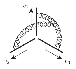
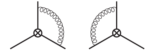
Figure 1: Two-loop Feynman graphs (top row) and one-loop counterterm diagrams (bottom row) contributing to the two-loop coefficient of the renormalization factor $\bm{Z}_{s}$.

The operator $\bm{O}_{s}$ is renormalized multiplicatively so that $\bm{O}_{s}\bm{Z}_{s}$ is UV finite. The anomalous dimension of this operator, which equals $6if^{abc}\,\bm{T}_{1}^{a}\bm{T}_{2}^{b}\bm{T}_{3}^{c}\,F_{1}(\beta_{12},\beta_{23},\beta_{31})$, can then be obtained from $\bm{Z}_{s}$ by using Eq. (1). To determine $\bm{Z}_{s}$, we need to separate the UV and IR divergences in the amplitude, for that we introduce an offshellness for the heavy quarks to regulate the IR divergences, while the UV divergences are regulated dimensionally.

The planar and counter-term diagrams in Figure 1 can be evaluated with standard techniques. The contribution to $F_{1}$ from those diagrams reads

$$F_{1}^{(2)\,\text{planar+CT}}=\frac{4}{3}\sum_{I,J,K}\epsilon_{IJK}\,\beta_{KI}\coth\beta_{KI}\\ \times\coth\beta_{IJ}\Bigg{[}\beta_{IJ}^{2}+2\beta_{IJ}\ln(1-e^{-2\beta_{IJ}})\\ -\operatorname{\mathrm{Li}}_{2}(e^{-2\beta_{IJ}})+\frac{\pi^{2}}{6}\Bigg{]}\,.$$

The diagram involving the triple-gluon vertex is the most technically challenging one. We have computed this diagram using a Mellin-Barnes representation with the result [19]

$$F_{1}^{(2)\,\text{non-planar}}=-\frac{4}{3}\sum_{I,J,K}\epsilon_{IJK}\beta_{IJ}^{2}\beta_{KI}\coth\beta_{KI}\,.$$

For Euclidean velocities, our result agrees numerically with a position-space-based integral representation derived in [27]. Combining all contributions, we find

$$F_{1}^{(2)}(\beta_{12},\beta_{23},\beta_{31})=\frac{4}{3}\sum_{I,J,K}\epsilon_{IJK}g(\beta_{IJ})r(\beta_{KI})\,,$$ (3)

where

$$r(\beta) =\beta\coth\beta\,,$$

$$g(\beta) =\coth\beta\Bigg{[}\beta^{2}+2\beta\ln(1-e^{-2\beta})$$

$$\hskip 30.00005pt-\operatorname{\mathrm{Li}}_{2}(e^{-2\beta})+\frac{\pi^{2}}{6}\Bigg{]}-\beta^{2}-\frac{\pi^{2}}{6}\,.$$ (4)

The function $f_{2}$ can be obtained from the above result by writing $w_{23}=-\sigma_{23}v_{2}\cdot p_{3}/m_{3}$, $w_{31}=-\sigma_{31}v_{1}\cdot p_{3}/m_{3}$ and taking the limit $m_{3}\to 0$ at fixed $v_{I}\cdot p_{3}$. In that way, we obtain

$$f_{2}^{(2)}\left(\beta_{12},\ln\frac{-\sigma_{23}v_{2}\cdot p_{3}}{-\sigma_{13}v_{1}\cdot p_{3}}\right)\\ =-4g(\beta_{12})\,\ln\frac{-\sigma_{23}v_{2}\cdot p_{3}}{-\sigma_{13}v_{1}\cdot p_{3}}\,.$$ (5)

Whether a factorization of the three-parton terms into two functions depending on only a single cusp angle persists at higher orders in $\alpha_{s}$ is an open question, but our results certainly suggest a hidden structure, which seems worthy of further exploration.

It is interesting to investigate the behavior of the two functions $F_{1}$ and $f_{2}$ in the limit where two velocities coincide. This is relevant, e.g., for the situation when two heavy quarks are produced nearly at rest. Contrary to naive expectations based on antisymmetry, the two functions don’t vanish in this limit. Instead, they tend to a finite value due to the presence of Coulomb singularities. On the other hand, in the limit when all the parton masses are small, both functions vanish like $(m_{I}m_{J})^{2}/s_{IJ}$, in accordance with a factorization theorem proposed in [29, 30].

4 Top quark pair production

Top quark pair production at hadron colliders is an important process in the standard model. It is also the simplest example which involves two heavy quarks where $F_{1}$ and $f_{2}$ can contribute. Therefore, as a first application, it is interesting to use our results in this case. In [18, 19] we have worked out the relevant anomalous dimension matrices for both $q\bar{q}\to t\bar{t}$ and $gg\to t\bar{t}$ partonic processes, and derived the IR poles in the two-loop amplitudes. For the $q\bar{q}$ channel, our results agree with the numerical ones from [31], with the analytic results for some of the color coefficients given in [32, 33], and with the results in the small-mass limit from [34]. For the $gg$ channel, results in the literature are available only in the small-mass limit [35], and we have checked the agreement of our exact results with this limiting case. Later at the RADCOR 2009 conference, M. Czakon claimed that they had confirmed our results in the $gg$ channel [36].

Given the knowledge of the anomalous dimension matrices, it is possible to derive approximate formulas beyond next-to-leading order for various differential cross sections as well as the total cross section for this process. This was done for the invariant mass distribution in [18] where all the threshold enhanced terms at NNLO were exactly predicted. In [19], these threshold enhanced terms were resummed to all orders in $\alpha_{s}$ at NNLL accuracy, where also the total cross section was computed by integrating over the invariant mass. Details about these two works are discussed by A. Ferroglia in this proceeding.

5 Conclusions

The IR divergences of scattering amplitudes in non-abelian gauge theories can be absorbed into a multiplicative renormalization factor, whose form is determined by an anomalous-dimension matrix in color space. For processes with only massless partons in the external states, a simple form of the anomalous-dimension matrix has been conjectured. Although a lot of supporting arguments were given, a rigorous proof is still lacking. When massive partons are involved, at two-loop order, the anomalous-dimension matrix contains pieces related to color and momentum correlations among three partons as long as at least two of them are massive. This information is encoded in two universal functions: $F_{1}$, describing correlations among three massive partons, and $f_{2}$, describing correlations among two massive and one massless parton. These two functions have been calculated analytically in [18, 19], and therefore the IR divergences of any two-loop scattering amplitude with arbitrary number of massive and massless external particles are completely understood. These results also provide the basis for a systematic resummation of Sudakov logarithms at NNLL order, and are relevant to a large class of interesting hadron collider processes and thus have important implications for precision measurements at the LHC. As first applications, we worked out the IR poles in the two-loop amplitudes for $q\bar{q}\to t\bar{t}$ and $gg\to t\bar{t}$ processes, derived an approximate NNLO formula for the invariant mass distribution as well as total cross section for top quark pair production at hadron colliders, and also resummed the threshold enhanced terms to all orders in $\alpha_{s}$ at NNLL accuracy.

References

- [1] J. C. Collins, D. E. Soper and G. Sterman, Adv. Ser. Direct. High Energy Phys. 5, 1 (1988) [arXiv:hep-ph/0409313].
- [2] G. Sterman, Nucl. Phys. B 281, 310 (1987).
- [3] S. Catani and L. Trentadue, Nucl. Phys. B 327, 323 (1989).
- [4] S. Catani, Phys. Lett. B 427, 161 (1998) [arXiv:hep-ph/9802439].
- [5] G. Sterman and M. E. Tejeda-Yeomans, Phys. Lett. B 552, 48 (2003) [arXiv:hep-ph/0210130].
- [6] S. M. Aybat, L. J. Dixon and G. Sterman, Phys. Rev. Lett. 97, 072001 (2006) [arXiv:hep-ph/0606254].
- [7] S. M. Aybat, L. J. Dixon and G. Sterman, Phys. Rev. D 74, 074004 (2006) [arXiv:hep-ph/0607309].
- [8] T. Becher and M. Neubert, Phys. Rev. Lett. 102, 162001 (2009) [arXiv:0901.0722 [hep-ph]].
- [9] T. Becher and M. Neubert, JHEP 0906, 081 (2009) [arXiv:0903.1126 [hep-ph]].
- [10] C. W. Bauer, S. Fleming, D. Pirjol and I. W. Stewart, Phys. Rev. D 63, 114020 (2001) [arXiv:hep-ph/0011336].
- [11] C. W. Bauer, D. Pirjol and I. W. Stewart, Phys. Rev. D 65, 054022 (2002) [arXiv:hep-ph/0109045].
- [12] M. Beneke, A. P. Chapovsky, M. Diehl and T. Feldmann, Nucl. Phys. B 643, 431 (2002) [arXiv:hep-ph/0206152].
- [13] E. Gardi and L. Magnea, JHEP 0903, 079 (2009) [arXiv:0901.1091 [hep-ph]].
- [14] L. J. Dixon, E. Gardi and L. Magnea, JHEP 1002, 081 (2010) [arXiv:0910.3653 [hep-ph]].
- [15] S. Catani, S. Dittmaier and Z. Trocsanyi, Phys. Lett. B 500, 149 (2001) [arXiv:hep-ph/0011222].
- [16] M. Neubert, Phys. Rept. 245, 259 (1994) [arXiv:hep-ph/9306320].
- [17] T. Becher and M. Neubert, Phys. Rev. D 79, 125004 (2009) [Erratum-ibid. D 80, 109901 (2009)] [arXiv:0904.1021 [hep-ph]].
- [18] A. Ferroglia, M. Neubert, B. D. Pecjak and L. L. Yang, Phys. Rev. Lett. 103, 201601 (2009) [arXiv:0907.4791 [hep-ph]].
- [19] A. Ferroglia, M. Neubert, B. D. Pecjak and L. L. Yang, JHEP 0911, 062 (2009) [arXiv:0908.3676 [hep-ph]].
- [20] V. Ahrens, A. Ferroglia, M. Neubert, B. D. Pecjak and L. L. Yang, Phys. Lett. B 687, 331 (2010) [arXiv:0912.3375 [hep-ph]].
- [21] V. Ahrens, A. Ferroglia, M. Neubert, B. D. Pecjak and L. L. Yang, arXiv:1003.5827 [hep-ph].
- [22] S. Catani and M. H. Seymour, Phys. Lett. B 378, 287 (1996) [arXiv:hep-ph/9602277].
- [23] S. Moch, J. A. M. Vermaseren and A. Vogt, Phys. Lett. B 625, 245 (2005) [arXiv:hep-ph/0508055].
- [24] M. Neubert, Eur. Phys. J. C 40, 165 (2005) [arXiv:hep-ph/0408179].
- [25] G. P. Korchemsky and A. V. Radyushkin, Nucl. Phys. B 283, 342 (1987).
- [26] N. Kidonakis, Phys. Rev. Lett. 102, 232003 (2009) [arXiv:0903.2561 [hep-ph]].
- [27] A. Mitov, G. Sterman and I. Sung, Phys. Rev. D 79, 094015 (2009) [arXiv:0903.3241 [hep-ph]].
- [28] A. Mitov, G. Sterman and I. Sung, arXiv:1005.4646 [hep-ph].
- [29] A. Mitov and S. Moch, JHEP 0705, 001 (2007) [arXiv:hep-ph/0612149].
- [30] T. Becher and K. Melnikov, JHEP 0706, 084 (2007) [arXiv:0704.3582 [hep-ph]].
- [31] M. Czakon, Phys. Lett. B 664, 307 (2008) [arXiv:0803.1400 [hep-ph]].
- [32] R. Bonciani, A. Ferroglia, T. Gehrmann, D. Maitre and C. Studerus, JHEP 0807, 129 (2008) [arXiv:0806.2301 [hep-ph]].
- [33] R. Bonciani, A. Ferroglia, T. Gehrmann and C. Studerus, JHEP 0908, 067 (2009) [arXiv:0906.3671 [hep-ph]].
- [34] M. Czakon, A. Mitov and S. Moch, Phys. Lett. B 651, 147 (2007) [arXiv:0705.1975 [hep-ph]].
- [35] M. Czakon, A. Mitov and S. Moch, Nucl. Phys. B 798, 210 (2008) [arXiv:0707.4139 [hep-ph]].
- [36] M. Czakon, arXiv:1001.3994 [hep-ph].