Local spin polarization of Landau levels under Rashba spin-orbit coupling

Abstract

We investigate the local spin polarization texture of Landau levels under Rashba spin-orbit coupling in bulk two-dimensional electron gas (2DEG) systems. In order to analyze the spin polarization as a function of two-dimensional coordinates within the 2DEG, we first solve the system eigenstates in the symmetric gauge. Our exact analytical wavefunction solutions are shown to be gauge invariant with solutions obtained in the commonly used Landau gauge. We illustrate the two-dimensional spatial spin profile for a single Landau level and suggest means to measure and utilize the local polarization in practice.

I Introduction

Spin dependent transport phenomena in low dimensional systems have attracted considerable attention in recent years because of their potential application in information processing and storage devices sa ; zutic ; awsch . A paradigmatic proposal is the spin field-effect-transistor which utilizes the gate-controllable nitta Rashba spin-orbit coupling (SOC) rashba1 ; rashba2 in two-dimensional electron gases (2DEGs) to control the spin rotation of electrons as they propagate across the device datta ; mireles ; fujita . The Rashba SOC results from the structural inversion asymmetry of the microscopic confinement potential formed at the interface of semiconductor heterostructures rashba1 ; rashba2 . There is much interest recently in 2DEG systems with SOC and external magnetic fields. By applying a perpendicular magnetic field to the 2DEG system, the SOC competes with Zeeman spin-splitting and this interplay leads to further modification of band structure and other interesting results. A few examples are resonant spin-Hall conductance shen ; shun due to induced degeneracies of Landau levels at certain values of magnetic field zhigang , modified magneto-optical transition spectrums yang , beating patterns in the density of states and longitudinal resistivity wang , and altered Hall conductance demikhovskii which differs from the quantized values in the integer quantum Hall (IQH) regime. We note that previous works (including all of the above) perform their analyses in the Landau gauge. While the use of the Landau gauge is perfectly valid due to gauge invariance, the form of the wavefunction in this gauge does not capture the natural, rotational symmetry of the eigenstates. For example, in the presence of Rashba SOC, the spin polarization of eigenstates exhibits interesting spatial textures whose features cannot adequately be reflected by the wavefunctions obtained in the Landau gauge. The study of the locally varying spin polarization within a 2DEG may have a number of interesting applications. For instance, a well-controlled spin texture with distinct spatial modulation may be used as a resolution test for surface spin probe techniques. Additionally, it may be possible, by means of some localized probes, to harness an efficient spin current source from spatial regions with high spin polarization. Here, the spatial separation of spins is reminiscent of the optical dispersion (spatial separation of optical frequencies) found in monochromators, suggesting that it may be used as a form of spin filter.
In this article, we theoretically study the local spin polarization of Landau levels in the presence of Rashba SOC within an infinite 2DEG. To do so, we first present analytical solutions of the eigenstates of the system in the rotationally isotropic symmetric gauge. We demonstrate the gauge equivalence of our solutions with previously known solutions obtained in the Landau gauge. Finally, we show the spatial distribution of the spin components of Landau level states in the presence of Zeeman and Rashba SOC effects.

II Theory

II.1 Landau levels in the symmetric gauge

We first solve the Landau level wavefunctions without the Rashba SOC and Zeeman interactions in the symmetric gauge i.e. the IQH states. The wavefunctions form an orthonormal set which we use as the basis functions in solving the complete system. Under an external vertical magnetic field $\mathbf{B}$, the Hamiltonian of a spinless and otherwise free electron in a 2DEG is written as $\mathcal{H}_{0}=\mathbf{\Pi}^{2}/2m_{e}$, where $\mathbf{\Pi}=\mathbf{p}+e\mathbf{A}$ is the covariant momentum under the vector potential $\mathbf{A}$ which satisfies $\text{curl }\mathbf{A}=\mathbf{B}$, $-e$ is the electron charge, and $m_{e}$ the effective electron mass. Fixing the magnetic field $\mathbf{B}$ does not uniquely determine the vector potential, i.e. there is a gauge freedom. For a magnetic field that is perpendicular to the plane of the 2DEG, pointing in the $\hat{z}$-direction by convention, the Landau (L) gauge is given by $\mathbf{A}^{L}=(-B_{z}y,0,0)$ whilst the symmetric (sym) gauge is given by $\mathbf{A}^{\text{sym}}=B_{z}/2(-y,+x,0)$, where $B_{z}$ is the magnetic flux density (in Tesla) of the external field and $x,y$ are spatial coordinates in the plane of the 2DEG. In the presence of a uniform magnetic field, the system exhibits both translational and rotational symmetry about the $\hat{z}$-axis. Under the Landau gauge, it is well known that the solutions to the Hamiltonian are of the form capri

$$\Psi^{L}_{n}(x,y)=\exp{(ik_{x}x)}\psi_{n}[(y-y_{0})/r)],$$ (1)

where $y_{0}=\hbar k_{x}/eB_{z}$ is the $y$ coordinate of the cyclotron center, $r=\sqrt{\hbar/eB_{z}}$ is the magnetic length and $\psi_{n}$ ($n$, an integer) are the normalized $n$th order Hermite polynomials. The wavefunction $\Psi^{L}_{n}(x,y)$ characterizes the $n$th discrete Landau level in the presence of a magnetic field, with corresponding quantized energy spectrum $E_{n}=\hbar\omega(n+\frac{1}{2})$. Although the choice of Landau gauge preserves the translational symmetry of the system, the rotational invariance is lost in Eq. (1). In describing the circular Landau orbits of electrons which form in the presence of $\mathbf{B}$ fields, it is more natural to use the rotationally isotropic symmetric gauge. The use of the symmetric gauge has been applied previously to analyze other systems exhibiting rotational symmetry, e.g. in 2D two-electron systems goro , and quantum dots (QDs) in 2D parabolic confinement potentials (see, for example, noboru ; davies ), and QDs in radially symmetric hard-wall potentials with SOC tsit , in the presence of magnetic fields. Under this choice of gauge, it is convenient to define the complex variable $z=x+iy$ to represent spatial coordinates within the 2DEG, and introduce the operators capri :

$$a^{\dagger}=\frac{r}{\sqrt{2}\hbar}(\Pi_{x}+i\Pi_{y})\text{, }a=\frac{r}{\sqrt{2}\hbar}(\Pi_{x}-i\Pi_{y}).$$ (2)

In analogy to the harmonic oscillator, the Hamiltonian can be rewritten in terms of $a$ and $a^{\dagger}$, i.e., $\mathcal{H}_{0}=\hbar\omega(a^{\dagger}a+\frac{1}{2})$ with angular frequency $\omega=eB_{z}/m_{e}$. The operators $a^{\dagger}$ and $a$ satisfy the usual bosonic commutation relations and act as raising and lowering operators on the system eigenfunctions, respectively. Through the raising operator, we can generate the system eigenfunctions in any level $n$, by starting with the ground state wavefunctions $n=0$ or the lowest Landau level (LLL). The LLL is characterized by $a\Psi_{n=0}(z)=0$, whose solutions are given by the normalized wavefunctions capri ; laughlin :

$$\Psi_{n=0,m}(z)=\frac{1}{\sqrt{2\pi r^{2}2^{m}m!}}\left(\frac{z^{*}}{r}\right)^{m}\exp{\left(-\frac{|z|^{2}}{4r^{2}}\right)},$$ (3)

where ^∗ denotes complex conjugation, and the quantum number $m$ denotes the angular momentum. The degeneracy of the above wavefunction in $m$ implies that one can construct general LLL wavefunctions of the form

$$\Psi_{n=0} \propto \left(\sum_{m}a_{m}(z^{*})^{m}\right)\exp{\left(-\frac{|z|^{2}}{4r^{2}}\right)}$$ (4)

$$= \text{(const)}f(z^{*})\exp{\left(-\frac{|z|^{2}}{4r^{2}}\right)},$$

where $f(z^{*})$ is any arbitrary analytic function of $z^{*}$. The normalized eigenfunctions for arbitrary $n$ and $m$ are given by

$$\Psi_{n,m}=\frac{1}{\sqrt{n!}}{a^{\dagger}}^{n}\Psi_{0,m}.$$ (5)

II.2 Landau levels with Rashba SOC and Zeeman coupling in the symmetric gauge

We introduce spin into the system which in the case of 2DEGs in heterostructures enters the Hamiltonian through the Zeeman coupling and Rashba SOC rashba1 ; rashba2 terms. We assume a narrow-gap heterostructure, in which the Rashba SOC term is the dominant contribution, while the Dresselhaus SOC term dressel can be neglected. The Zeeman coupling and the Rashba SOC effects are, respectively, described by the matrix operators $\mathcal{H}_{Z}=g\mu B_{z}\sigma_{z}$, and $\mathcal{H}_{R}=\alpha/\hbar(\Pi_{y}\sigma_{x}-\Pi_{x}\sigma_{y})$, where $g$ is the Landé factor of electrons, $\mu=e\hbar/2m$ is the Bohr magneton, $\sigma_{i=x,y,z}$ are the Pauli spin matrices and $\alpha$ is the Rashba SOC parameter. In terms of the raising and lowering operators, the Rashba Hamiltonian has the compact form

$$\mathcal{H}_{R}=\frac{\sqrt{2}\alpha i}{r}\left(\begin{array}[]{cc}0&a\\ -a^{\dagger}&0\end{array}\right).$$ (6)

We solve the total Hamiltonian $\mathcal{H}=\mathcal{H}_{0}+\mathcal{H}_{R}+\mathcal{H}_{Z}$ for its eigenspinors, $\mathbf{\Psi}_{n,m}(z)=\left(\Psi_{n,m}^{\uparrow}(z),\Psi_{n,m}^{\downarrow}(z)\right)^{\text{T}}$, by writing the spinor components as a linear combination of the spinless and normalized eigenfunctions given by Eq. (5),

$$\mathbf{\Psi}_{N,m}(z)=\sum_{n=0}^{N}\Psi_{n,m}(z)\left(\begin{array}[]{c}a_{n}^{\uparrow}\\ a_{n}^{\downarrow}\end{array}\right),$$ (7)

where $a_{n}^{\uparrow(\downarrow)}$ denotes the up (down) spin coefficient of the $n$th Landau level, and we use the vector notation $\mathbf{\Psi}$ to denote eigenspinor solutions. Note that in Eq. (7) the summation runs over the Landau level index $n$ whilst the angular momentum $m$ is kept constant . The Schrödinger equation $(\mathcal{H}-E\mathbf{I})\mathbf{\Psi}_{N,m}=\mathbf{0}$ ($\mathbf{I}$ is the 2-by-2 identity matrix) then reads

$$\left(\begin{array}[]{cc}(\hbar\omega(a^{\dagger}a+\frac{1}{2})+g\mu B_{z}-E)\sum_{n=0}^{N}a_{n}^{\uparrow}\Psi_{n,m}+\frac{\sqrt{2}\alpha i}{r}a\sum_{n=0}^{N}a_{n}^{\downarrow}\Psi_{n,m}\\ -\frac{\sqrt{2}\alpha i}{r}a^{\dagger}\sum_{n=0}^{N}a_{n}^{\uparrow}\Psi_{n,m}+(\hbar\omega(a^{\dagger}a+\frac{1}{2})-g\mu B_{z}-E)\sum_{n=0}^{N}a_{n}^{\downarrow}\Psi_{n,m}\end{array}\right)=\mathbf{0}.$$ (8)

To simplify Eq. (8) we utilize the orthogonality of the Landau level wavefunctions, namely that $\langle\Psi_{n,m}|\Psi_{n^{\prime},m}\rangle=\delta_{n,n^{\prime}}$ for any value of $m$. Let us denote as $\mathbf{M}$ the column vector on the left hand side of Eq. (8). Now, we consider multiplying both sides of Eq. (8) by the state-bra $\langle\Psi_{s,m}|$, which yields the equation $\int_{\mathbb{C}}\Psi_{s,m}^{*}(z)\mathbf{M}d^{\text{ }2}z=\mathbf{0}$, where the integration is performed over the entire complex space $\mathbb{C}$. After canceling the orthogonal terms and applying the raising and lowering operators, Eq. (8) is simplified as

$$\left(\begin{array}[]{cc}(\hbar\omega(s+\frac{1}{2})+g\mu B_{z}-E)a_{s}^{\uparrow}+\frac{\sqrt{2}\alpha i}{r}a_{s+1}^{\downarrow}\sqrt{s+1}\\ -\frac{\sqrt{2}\alpha i}{r}a_{s-1}^{\uparrow}\sqrt{s}+(\hbar\omega(s+\frac{1}{2})-g\mu B_{z}-E)a_{s}^{\downarrow}\end{array}\right)=\mathbf{0}.$$ (9)

The resulting equation is a simple system of two equations relating the spinor components of state $s$ and its adjacent states $s\pm 1$. Therefore, we can replace $s\rightarrow s-1$ without any loss of generality in the top row of Eq. (9), to yield a regular eigenvalue equation whose energy eigenvalues $E$ are

$$E^{\pm}=s\hbar\omega\pm\sqrt{\xi^{2}+2s(\alpha/r)^{2}}$$ (10)

where $\xi=\hbar\omega/2-g\mu B_{z}$. In particular, $\xi$ is the energy of the LLL with eigenspinors $(a_{s-1}^{\uparrow},a_{s}^{\downarrow})^{\text{T}}=(0,1)^{\text{T}}$. Compared to the energy spectrum of pure Landau levels, the LLL energy differs only by the Zeeman term $-g\mu B_{z}$ corresponding the electron spins pointing antiparallel to the applied magnetic field. Furthermore, in the LLL the wavefunctions do not experience any spin splitting from the Zeeman term (since all eigenstates are spin down, $\sigma_{z}=-1$) and the wavefunctions are completely independent of the Rashba SOC in the system. In general, when $s\neq 0$, the Zeeman and Rashba SO coupling breaks the spin degeneracy and the wavefunctions are highly dependent on the SOC. Let us label the spin-split states $\mathbf{\Psi}_{s,m}^{\pm}$, such that $\mathcal{H}\mathbf{\Psi}_{s,m}^{\pm}=E_{s}^{\pm}\mathbf{\Psi}_{s,m}^{\pm}$. The eigenspinor solutions are given by

$$\mathbf{\Psi}_{s,m}^{\pm}=N_{s}^{\pm}\left(\begin{array}[]{c}\kappa_{s}^{\pm 1}\Psi_{s-1,m}\\ \Psi_{s,m}\end{array}\right),$$ (11)

where $\kappa_{s}=\frac{i\alpha\sqrt{2s}/r}{\xi+\sqrt{\xi^{2}+2s(\alpha/r)^{2}}}$, and $N_{s}^{\pm}$ are the normalization constants. Since the basis wavefunctions $\{\Psi_{s,m}\}$ are normalized, $N_{s}^{\pm}$ satisfies $|N_{s}^{\pm}|=1/\sqrt{|\kappa_{s}^{\pm 1}|^{2}+1}$. Once again, we find that the Landau levels are infinitely degenerate since the choice of $m$ does not affect the energy eigenvalue. Therefore, taking arbitrary linear combinations in $m$ of the wavefunctions yield general solutions as before:

$$\mathbf{\Psi}_{s}^{\pm}=N\sum_{m}a_{m}\left(\begin{array}[]{c}\kappa_{s}^{\pm}\Psi_{s-1,m}\\ \Psi_{s,m}\end{array}\right),$$ (12)

where the normalization constant is determined by the requirement $\langle\mathbf{\Psi}_{s}^{\pm}|\mathbf{\Psi}_{s}^{\pm}\rangle=1$, i.e. $|N|=\left(\sum_{m}|a_{m}|^{2}\right)^{-1/2}$ $\left(|\kappa_{s}^{\pm}|^{2}+1\right)^{-1/2}$.

II.3 Gauge invariance

We demonstrate gauge invariance of our solutions obtained in the symmetric gauge with respect to the wavefunctions in the Landau gauge. The U(1) gauge invariance of electromagnetism requires that for a gauge transformation, $\mathbf{A}^{\text{ }^{\prime}}=\mathbf{A}+\nabla\chi$, the electron wavefunction must undergo a corresponding transformation,

$$\psi^{{}^{\prime}}=U\psi=\exp{\left(-\frac{ie}{\hbar c}\chi\right)}\psi,$$ (13)

in order for the Schrödinger equation to remain invariant in form. In other words the electrons acquire an extra phase factor due to the gauge transformation, which implies that physical observables are identical in both gauges. In going from the Landau to the symmetric gauge, the required gauge transformation is given by

$$\chi=\frac{B_{z}xy}{2}.$$ (14)

For simplicity, we illustrate the principle for only the $s=1$ eigenstates. Without any loss of generality, we can focus on the eigenfunctions that have their cyclotron centres at the origin of the system of coordinates, $(x_{0},y_{0})=\mathbf{0}$. Under these set of conditions, the normalized eigenfunctions in the Landau gauge have form wang ; tan :

$$\mathbf{\Psi}^{L}(x,y)=\frac{N}{\sqrt{\sqrt{\pi}r}}\left(\begin{array}[]{c}\kappa_{s=1}^{\pm}\\ \sqrt{2}y/r\end{array}\right)\exp{\left(-\frac{y^{2}}{2r^{2}}\right)},$$ (15)

On the other hand, considering Eqs. (4), (5) and (11), the general $s=1$ wavefunctions in the symmetric gauge are of the form

$$\mathbf{\Psi}^{\pm}(z)=N\left(\begin{array}[]{c}\kappa_{1}^{\pm 1}f(z^{*})\exp{\left(-\frac{|z|^{2}}{4r^{2}}\right)}\\ (2\partial_{z^{*}}-z/2r^{2})\left[f(z^{*})\exp{\left(-\frac{|z|^{2}}{4r^{2}}\right)}\right]\end{array}\right)$$ (16)

Note that Eq. (16) is obtained after normalizing $\Psi_{0}(z)$ and $a^{\dagger}\Psi_{0}(z)$, and substituting the explicit expression for the $a^{\dagger}$ operator. Now, gauge invariance is valid if the same wavefunctions in the respective gauges are linked via the relation of Eq. (13). It therefore suffices to construct a wavefunction in the symmetric gauge—via the analytic function $f(z^{*})$—for which this holds. Consider

$$f(z^{*})=\exp{\left(\frac{z^{*2}}{4r^{2}}\right)}=\sum_{k=0}^{\infty}\frac{1}{k!}\left(\frac{z^{*2}}{4r^{2}}\right)^{k}.$$ (17)

Substituting this choice of $f$ into our symmetric gauge solution, we obtain after some manipulation

$$\mathbf{\Psi}^{\pm}(x,y)=N\left(\begin{array}[]{c}\kappa_{1}^{\pm 1}\eta^{\uparrow}\exp{\left(\frac{-y^{2}-ixy}{2r^{2}}\right)}\\ -\frac{2iy}{r^{2}}\eta^{\downarrow}\exp{\left(\frac{-y^{2}-ixy}{2r^{2}}\right)}\end{array}\right)$$ (18)

where $\eta^{\uparrow(\downarrow)}$ is the normalization coefficient for the up (down) spin branch of the spinor. For $\Psi_{0}(z)$ in the up-spin branch to be correctly normalized, we require $\eta^{\uparrow}=\sqrt{\sqrt{\pi}r}$. On the other hand, in the down-spin branch we set $\eta^{\downarrow}=i\sqrt{r/\left(2\sqrt{\pi}\right)}$ to satisfy normalization for $a^{\dagger}\Psi_{0}(z)$. This then yields for our symmetric gauge wavefunction

$$\mathbf{\Psi}^{\pm}(x,y) = \frac{N}{\sqrt{\sqrt{\pi}r}}\left(\begin{array}[]{c}\kappa_{1}^{\pm 1}\\ \sqrt{2}y/r\end{array}\right)\exp{\left(\frac{-y^{2}}{2r^{2}}\right)}\exp{\left(\frac{-ixy}{2r^{2}}\right)},$$ (21)

which is just the wavefunction in the Landau gauge multiplied by the gauge transformation phase factor:

$$\mathbf{\Psi}^{\pm}(x,y)=\mathbf{\Psi}^{L}(x,y)\exp{\left(\frac{-ie\chi}{\hbar}\right)}.$$ (22)

III Numerical simulations of local spin polarization

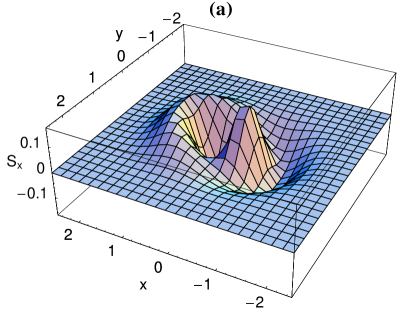
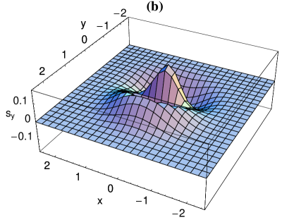
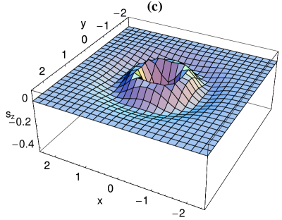
Figure 1: (color online) Local spatial distribution of spin polarization of $(s=1;m=1;+)$ level obtained in the symmetric gauge, $\langle\mathbf{\Psi}_{s=1,m=1}^{+}|\sigma_{i}|\mathbf{\Psi}_{s=1,m=1}^{+}\rangle$. The spatial coordinates are in arbitrary units. The $x$ and $y$ spin components, shown in (a) and (b) respectively, arise directly from the Rashba spin-orbit coupling. In (c) the spin polarization along the $z$ direction due to the Zeeman coupling is shown.

We present some numerical results based on the eigenspinors we derived for the symmetric gauge. In Fig. 1 we plot the local, spatial spin polarization $\langle\mathbf{\Psi}_{s,m}^{\pm}|\sigma_{i}|\mathbf{\Psi}_{s,m}^{\pm}\rangle$ for the $(s=1;m=1;+)$ level in the symmetric gauge in the 2DEG plane. First of all, we notice that the spin distributions are circular in nature, reflecting the spatial probability density distribution of the Landau orbits. Of the $x,y,z$-spin components, the most interesting are the in-plane $x$ and $y$ components [Figs. 1(a) and (b) respectively] as these components arise from the Rashba SOC. For the Rashba Hamiltonian $\mathcal{H}_{R}$, the effective magnetic field $\mathbf{\Omega}(\mathbf{k})$ is oriented in the plane of the 2DEG, and is orthogonal to the in-plane momentum $\mathbf{k}_{\parallel}$, i.e. $\mathbf{\Omega}(\mathbf{k})\cdot\mathbf{k}_{\parallel}=0$. The spin alignment along $\mathbf{\Omega}(\mathbf{k})$ can be seen in Fig. 1, if one imagines an electron moving in a circular orbit around the origin with a tangential velocity of $\mathbf{v}=\hbar\mathbf{k}_{\parallel}/m_{e}$. Thus, the results of our quantum mechanical analysis are in general agreement with the classical picture. The $z$-component of the spin, on the other hand, shown in Fig. 1(c) is uniform along the orbit, as it arises from the $\mathbf{k}$-independent Zeeman coupling. For the opposite eigenstate $(s=1;m=1;-)$, the values of the $x$ and $y$-spin components have opposite sign. The $z$-components, however, are not related by any simple transformation, although the general shape of the spatial distributions is the same. Increasing $m$, one observes an increase in the radius of the circular distributions. Finally, the Landau level index $s$ defines the maximum number of concentric circular orbits in the electron probability distribution. Therefore, the electron states in the higher Landau levels are characterized by a larger number of “ripples” in their spin texture. In practice, this spatial modulation of the spin polarization can be characterized by means of quantum point contacts (QPC) rokhinson , as the spatial resolution of this technique ($\sim 100$ nm) is comparable to the Landau orbital radii. In particular, one could conceive a magnetic-focusing arrangement whereby two QPCs are separated in space by twice the cyclotron radius. The first QPC behaves as an electron source, whilst the other serves as the collector. Under the influence of the magnetic field, electrons from the source follow a semi-circular trajectory in the 2DEG with a cyclotron radius, $r_{c}=\hbar k_{F}/eB$ ($k_{F}$ is the Fermi wavevector of electrons in the source QPC) and are collected by the detector. This technique has been used previously to image the trajectory of cyclotron orbits in 2DEG systems in the presence of a vertical magnetic field crook ; aidala . Additionally, we have shown that the momentum-dependent SOC field manifests itself as a spatially non-uniform in-plane spin-polarization along the electron orbits. This spatial variation may be detected experimentally through the use of magneto-optical techniques such as polarized absorption spectroscopy aifer , magneto-optical Kerr rotation kikk or magneto-reflectivity measurements chug . A probe-based QPC technique could also be used to tap the spin-current from the system locally (assuming that it does not introduce significant local perturbations to the system). By placing the probe at optimal positions corresponding to the peak polarization values, we could conceivably draw a highly spin-polarized current, thus implementing an efficient spin filtering scheme.
In summary, we studied the spatial spin polarization texture of Landau levels in the presence of Rashba SOC. To do so we solved the wavefunctions for the system in the symmetric gauge, demonstrating the gauge invariance of our solutions with previously known solutions in the Landau gauge. The two-dimensional analysis of the spatial spin dispersion may be important for several reasons (i) the momentum-dependent spin-orbit coupling effect is clearly seen in the Landau orbits (see Fig. 1), and this unifies the quantum mechanical and classical pictures, (ii) the theoretically predicted spatial spin distribution may readily be verified experimentally using standard magnetic-focusing techniques, and (iii) it may find useful applications in spintronics, such as efficient spin filtering devices and sources of spin polarized current.

References

References

- (1) Wolf S A, Awschalom D D, Buhrman R A, Daughton J M, von Molnar S, Roukes M L, Chtchelkanova A Y and Treger D M 2001 Science 294 1488
- (2) Žutić I, Fabian J and Sarma S D 2004 Rev. Mod. Phys. 76 323
- (3) Awschalom D D, Loss D and Samarth N (ed) 2002 Semiconductor Spintronics and Quantum Computing (Berlin: Springer)
- (4) Nitta J, Akazaki T, Takayanagi H and Enoki T 1997 Phys. Rev. Lett. 78 1335
- (5) Rashba E I 1960 Fiz. Tverd. Tela (Leningrad) 2 1224 [1960 Sov. Phys. Solid State 2 1109]
- (6) Bychkov Y A and Rashba E I 1984 J. Phys. C 17 6039
- (7) Datta S and Das B 1990 Appl. Phys. Lett. 56 665
- (8) Mireles F and Kirczenow G 2001 Phys. Rev. B 64 024426
- (9) Fujita T, Jalil M B A and Tan S G 2008 J. Phys.: Condens. Matter 20 115206
- (10) Shen S -Q, Bao Y -J, Ma M, Xie X C, and Zhang F C 2005 Phys. Rev. B 71 155316
- (11) Shen S -Q, Ma M, Xie X C, and Zhang F C 2004 Phys. Rev. Lett. 92 256603
- (12) Wang Z and Zhang P 2007 Phys. Rev. B 75 233306
- (13) Yang C H, Xu W and Tang C S 2007 Phys. Rev. B 76 155301
- (14) Wang X F and Vasilopoulos P 2003 Phys. Rev. B 67 085313
- (15) Demikhovskii V Ya and Perov A A 2007 Phys. Rev. B 75 205307
- (16) Goroshchenko S Ya and Ukrainskii I I 1988 Phys. Stat. Sol. (b) 145 187
- (17) Miura N 2008 Physics of Semiconductors in High Magnetic Fields (Oxford University Press)
- (18) Davies J H 1998 The Physics of Low-dimensional Semiconductors: An Introduction (Cambridge University Press)
- (19) Tsitsishvili E, Lozano G S and Gogolin A O, preprint: cond-mat/0310024 (October 2003)
- (20) Capri A Z 1985 Nonrelativistic Quantum Mechanics (California: Benjammin/Cummings)
- (21) Laughlin R B 1983 Phys. Rev. Lett. 50 1395
- (22) Dresselhaus G 1955 Phys. Rev. 100 580
- (23) Tan S G, Jalil M B A, Teo K L and Liew T 2005 J. Appl. Phys. 97 10A716
- (24) Rokhinson L P, Larkina V, Lyanda-Geller Y B, Pfeiffer L N and West K W 2004 Phys. Rev. Lett. 93 146601
- (25) Crook R, Smith C G, Simmons M Y and Ritchie D A 2000 Phys. Rev. B 62 5174
- (26) Aidala K E, Parrott R E, Kramer T, Heller E J, Westervelt R M, Hanson M P and Gossard A C 2007 Nature Phys. 3 464
- (27) Aifer E H, Goldberg B B, Broido D A 1996 Phys. Rev. Lett. 76 680
- (28) Kikkawa J M, Smorchkova I P, Samarth N, Awschalom D D 1997 Science 277 1284
- (29) Chughtai R, Zhitomirsky V, Nicholas R J and Henini M, pre-print: cond-mat/0111492 (November 2001)