Hot Stars with Hot Jupiters Have High Obliquities

Abstract

We show that stars with transiting planets for which the stellar obliquity is large are preferentially hot ($T_{\rm eff}~{}>~{}6250$ K). This could explain why small obliquities were observed in the earliest measurements, which focused on relatively cool stars drawn from Doppler surveys, as opposed to hotter stars that emerged later from transit surveys. The observed trend could be due to differences in planet formation and migration around stars of varying mass. Alternatively, we speculate that hot-Jupiter systems begin with a wide range of obliquities, but the photospheres of cool stars realign with the orbits due to tidal dissipation in their convective zones, while hot stars cannot realign because of their thinner convective zones. This in turn would suggest that hot Jupiters originate from few-body gravitational dynamics, and that disk migration plays at most a supporting role.

1. Introduction

There are now 28 cases of stars with transiting planets for which the stellar obliquity—or more precisely its sky projection—has been measured via the Rossiter-McLaughlin effect. The history of these measurements is perplexing. Starting with the pioneering measurement of Queloz et al. (2000), for 8 years a case was gradually building that the orbits of hot Jupiters are always well-aligned with the rotation of their parent stars. Then in a sudden reversal, several misaligned systems were found, with the first sighting by Hébrard et al. (2008) and the most recent spate of discoveries by Triaud et al. (2010).

In this Letter we point out that the misaligned systems are preferentially those with the hottest photospheres. In § 2 we discuss the sample, and in § 3 we display the patterns involving the order in which the measurements were made, the stellar effective temperature, and the stellar obliquity. In § 4 we speculate on the meaning of the patterns, and in § 5 we summarize the results and their implications for theories of the origin of hot Jupiters.

2. The Sample

We focused on those systems for which the projected spin-orbit angle, $\lambda$, was measured with a 1$\sigma$ precision of $10^{\circ}$ or better. The less precise cases are not as helpful because we cannot tell definitively whether the system is aligned or misaligned, and because the large uncertainties are usually associated with strong systematic effects.

We omitted Kepler-8 (Jenkins et al. 2010) from consideration even though the quoted uncertainty is smaller than $10\arcdeg$, because no data were gathered immediately before or after the transit, precluding tests for a systematic velocity offset on the transit night. Such offsets are possible, or even probable, for stars as faint as Kepler-8 observed in bright moonlight (see, e.g., Tripathi et al. 2010). When we reanalyzed the Kepler-8 data allowing for such an offset, the result was $\lambda=20^{\circ}\pm 20^{\circ}$.

Table 1 summarizes the resulting sample of 19 systems, along with the properties of the 9 omitted systems, for completeness. For simplicity we refer to the planets as “hot Jupiters” because they are all giant planets with short periastron distances, although it should be remembered that they span a wide range of masses (0.36–11.8 $M_{\rm Jup}$) and orbital periods (1.3–111 d).

3. The Pattern

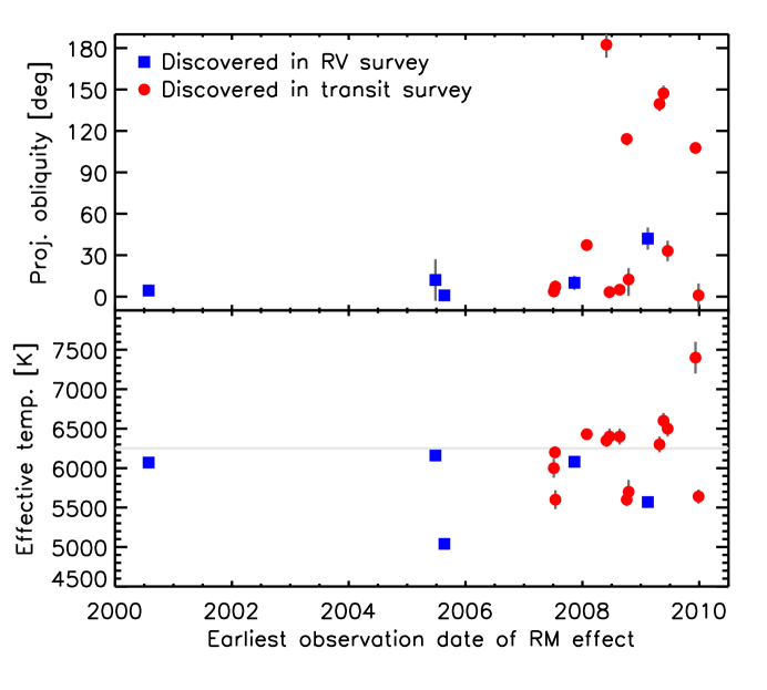
Figure 1.— A brief history of Rossiter-McLaughlin measurements. Top.—The projected obliquity (spin-orbit angle) is plotted as a function of the earliest date of observation reported in the literature. Blue squares indicate systems discovered by RV surveys, while red circles indicate systems found in photometric transit surveys. Bottom.—The stellar effective temperature of the same systems. Systems with $T_{\rm eff}$ higher than 6250 K have been discovered by transit surveys, and began to be examined for the RM effect in 2008.

The top panel of Fig. 1 shows $\lambda$ as a function of the date of the earliest reported observation of the Rossiter-McLaughlin effect. The trend of low values (good alignment) for the first few years is evident, as is the “spike” of high values (misalignment) in the most recent years. This plot also suggests that the systems initially discovered in radial-velocity (RV) surveys are systematically more well-aligned than those systems discovered in transit surveys.

The reason for this pattern may be that the earlier measurements focused on cooler and less massive stars. The bottom panel of Fig. 1 shows that the average effective temperature ($T_{\rm eff}$) of the host stars has risen with time. Only in 2008 did investigators begin examining stars with $T_{\rm eff}>6250$ K, and all of those systems were identified in transit surveys as opposed to RV surveys.

We cannot give a deterministic explanation for this trend, as it depends not only on the selection functions for the various surveys but also sociological factors affecting the allocation of telescope time. However it seems probable that cooler stars were examined earlier because they allow for better RV precision, and therefore greater ease of confirming the existence of planets. Indeed, most RV surveys exclude early-type stars altogether. In contrast, transit surveys have nearly magnitude-limited samples that include hot and luminous stars. These factors may explain why planets around hot stars were only found in transit surveys, and why they emerged relatively late from those surveys.

Fig. 2 shows $\lambda$ as a function of $T_{\rm eff}$. Most of the misaligned systems are around the hottest stars in the sample. The transition from aligned to misaligned occurs around $T_{\rm eff}=6250$ K (spectral type F8), which for the rest of this Letter we take to be the boundary between “cool” and “hot” stars. We will also use the term “misaligned” to mean $|\lambda|>10^{\circ}$ with $>$3$\sigma$ confidence.

Among the cool stars, two out of 11 (18%) are misaligned, while among the hot stars, 6 out of 8 (75%) are misaligned. Another way to describe the pattern is to enumerate exceptions to the rule that only hot stars are misaligned. There are two types of exceptions: “strong” exceptions in which a cool star is misaligned, and “weak” exceptions in which a hot star is apparently well-aligned. Weak exceptions are not as serious because only the sky-projected obliquity is measured, and consequently a low value of $\lambda$ could be observed for a misaligned system. Out of 19 systems, there are two strong exceptions and two weak exceptions.

Figure 2.— Misaligned systems have hotter stars. Top.—The projected obliquity is plotted against the effective temperature of the host star. A transition from mainly-aligned to mainly-misaligned seems to occur at $T_{\rm eff}\approx 6250$ K. The two strongest exceptions are labeled. Symbol colors and shapes have the same meaning as in Fig. 1. Bottom.—The mass of the convective zone of a main-sequence star as a function of $T_{\rm eff}$, from Pinsonneault, DePoy, & Coffee (2001). It is suggestive that 6250 K is approximately the temperature at which the mass of the convective zone has bottomed out.

Many seemingly compelling trends of this kind turn out to be spurious. The best way to make progress is to gather more data. The prediction that misaligned systems are preferentially around hot stars will be tested in the near future, and a primary purpose of this Letter is to enunciate the prediction in advance of forthcoming observations.

It is also important to consider selection effects. From a transit surveyor’s perspective, the most important difference between a well-aligned star and a misaligned star of the same spectral type is that the well-aligned star has a larger $v\sin i$ (sky-projected rotation rate). A large $v\sin i$ implies broader spectral lines and poorer Doppler precision, inhibiting planet discovery. Therefore there is a potential bias against discovering well-aligned systems. We must ask whether there could exist a large population of well-aligned systems around hot stars that has been missed by current surveys.

For this question, the RV surveys are irrelevant because they exclude all hot stars regardless of $v\sin i$. As for the transit surveys, to assess the bias we must know how transit candidates are identified and followed up. Latham et al. (2009) provided a complete inventory of transit candidates and follow-up observations, which we take to be representative. They chose 28 transit candidates for spectroscopic follow-up, without regard to spectral type. Of those, 4 were not pursued further once it was found that $v\sin i>50$ km s^-1. The other 24 cases were observed assiduously until a hot Jupiter was confirmed (2 cases) or ruled out (22 cases). Hence, any bias against well-aligned systems is probably only for stars with $v\sin i\lower 2.15277pt\hbox{$\;\buildrel>\over{\sim}\;$}50$ km s^-1. Such rapid rotators typically have spectral types $<$F3 and $T_{\rm eff}>6700$ K, whereas our sample ranges from 5040 to 6700 K, with one exception. Hence it seems unlikely that this bias is completely responsible for the observed $\lambda$-$T_{\rm eff}$ relation, although it may play some role.

Another caveat is that we cannot tell whether the relevant parameter is really $T_{\rm eff}$ or some other correlated variable, such as stellar mass. The transition temperature of 6250 K corresponds to approximately 1.3 $M_{\odot}$ for solar-metallicity main-sequence stars.

4. Possible Explanations

Despite these caveats it is impossible to resist speculating on the reasons why hot stars with hot Jupiters have high obliquities. We restrict ourselves to an airing of issues and a toy model illustrating a speculative hypothesis, leaving detailed investigations for future work.

One possibility is that there are two pathways for producing hot Jupiters, one of which is specific to low-mass stars and yields low obliquities, while the other occurs mainly for massive stars and produces a broad range of obliquities. The low-obliquity mechanism could be inspiral due to tidal interactions with the protoplanetary disk (Lin, Bodenheimer, & Richardson 1996). The high-obliquity mechanism could be some combination of planet-planet scattering (Chatterjee et al. 2008) and Kozai cycles (Fabrycky & Tremaine 2007). It is not obvious why these mechanisms would have a strong dependence on stellar mass or temperature, although it is interesting that 1.3 $M_{\odot}$ is approximately the same stellar mass above which giant planets are found to have larger masses, wider orbits, and a higher rate of occurrence (Bowler et al. 2010). Perhaps more massive stars are more likely to form systems of massive planets in unstable configurations, leading to an enhanced rate of gravitational scattering in comparison to cooler stars.

Another possibility is suggested by the sharpness of the transition from aligned to misaligned, and its location at $T_{\rm eff}\approx 6250$ K. For main-sequence stars, this is approximately the temperature above which the mass in the outer convective zone ($M_{\rm cz}$) becomes inconsequential. The decline in $M_{\rm cz}$ is illustrated in the bottom panel of Fig. 2, based on the relation presented by Pinsonneault, DePoy, & Coffee (2001). Between spectral types G0 and F5 (5940 and 6650 K), $M_{\star}$ increases by a factor of 1.3, and $M_{\rm cz}$ decreases by a factor of 120.

Convective zones are important for the production of magnetic fields and for tidal dissipation. Magnetic fields may be relevant by setting the inner radius of the protoplanetary gas disk, where accreting material is captured onto field lines, or by allowing the star to spin down through magnetic braking. The possible relevance of tidal dissipation is even more obvious, as it would tend to realign the star with the orbit.

Pursuing this latter point, we hypothesize that there is a single mechanism for producing hot Jupiters, and this mechanism yields a broad range of obliquities. For the cool stars, tidal dissipation damps the obliquity within a few Gyr, while for the hot stars, dissipation is ineffective. Therefore we observe hot Jupiters to be well-aligned around cool stars, and misaligned around hot stars.

It has been argued previously that tidal dissipation is too slow to affect the stellar spin state (see, e.g., Winn et al. 2005), but these arguments should now be reconsidered. The timescales for tidal dissipation are not understood from first principles and are poorly constrained by observations. Another objection is that obliquity damping should be accompanied by spin-orbit synchronization, which is not observed. However, cool stars spin down due to magnetic braking. Thus, even if tides do synchronize the rotation and orbital periods while damping the obliquity, magnetic braking could subsequently slow the rotation to the observed values. A third objection, and the hardest to overcome, is that obliquity damping is accompanied by orbital decay, threatening the planet with engulfment (Levrard, Winisdoerffer, & Chabrier 2009, Barker & Ogilvie 2009). The planet must surrender all its angular momentum in order to reorient the star, because of the star’s large moment of inertia.

We are thereby led to explore a scenario in which the star’s moment of inertia is drastically reduced. We suppose that only the convective zone is dissipatively torqued by the planet, and that the radiative zone is weakly coupled to the convective zone and to the planet. Without the burden of the massive radiative interior, the convective zone—and thus the observable photosphere—can align with the planetary orbit without drawing in the planet. Likewise, the magnetic braking torque would be even more effective in slowing the surface rotation speed and preventing spin-orbit synchronization.

Core-envelope decoupling has been discussed in the context of young stars (see, e.g., Irwin & Bouvier 2009), but here we would need decoupling to persist for a sizable fraction of the main-sequence lifetime of a cool star. A problem with this notion is that the Sun’s convective and radiative zones appear to be well-coupled (Howe 2009). However, this may not have always been so, and it was not a foregone conclusion theoretically (see, e.g., Pinsonneault et al. 1989). The most plausible solar coupling mechanisms, magnetic linkage and internal gravity waves, may be absent or may act on longer timescales for stars with hot Jupiters.

To investigate the effects of core-envelope decoupling we used the equations of Eggleton & Kiseleva-Eggleton (2001) to follow a circular orbit of a hot Jupiter around a 1 $M_{\odot}$ star, with initial periods $P_{\rm orb}=3$ d and $P_{\rm rot}=10$ d. Based on the stellar evolution code EZ-Web we take the convective zone to have mass $0.015~{}M_{\odot}$, moment of inertia $0.0066$ $M_{\odot}R_{\odot}^{2}$, and apsidal motion constant $9\times 10^{-4}$. We chose a tidal dissipation factor $Q^{\prime}_{\star}=6\times 10^{6}$, which is consistent with the current population of hot Jupiters, although the large uncertainty in $Q^{\prime}_{\star}$ causes a correspondingly large uncertainty in all of the timescales reported here. We do not model the dissipative shear or the non-dissipative oblateness coupling between the convective zone and the radiative interior. The magnetic braking torque was modeled with an extra term in the equations of motion:

$$\frac{d\vec{\Omega}_{\star}}{dt}=-\alpha_{\rm mb}\Omega_{\star}^{2}\vec{\Omega}_{\star}.$$ (1)

For the braking coefficient $\alpha_{\rm mb}$ we used $1.66\times 10^{-13}$ yr, based on a scaling of the Barker & Ogilvie (2009) results according to the moment of inertia.

Fig. 3 shows the time history of $P_{\rm rot}$, $P_{\rm orb}$, and the stellar obliquity $\psi$, assuming an initial value of 60 deg. (Similar results were obtained from an initially retrograde condition.) Three lines are plotted, corresponding to planet masses of 3, 1, or 1/3 $M_{\rm Jup}$. For Jupiter-mass planets, the stellar obliquity damps before the planet is consumed. Magnetic braking prevents synchonization of the convective zone with the orbit, in agreement with observations. However, this model also implies that orbits decay within main-sequence lifetimes, and that close-in massive planets should be rarer around cool stars than hot stars, due to their more rapid orbital decay.

Another prediction is that the planets exerting the weakest tidal torques should be seen as “strong exceptions”: misaligned planets around cool stars. To compute the obliquity-damping component of the tidal torque we averaged together the last terms of Eqns. (10) and (11) of Eggleton & Kiseleva-Eggleton (2001), giving a decay timescale proportional to

$$\left(\frac{M_{\rm cz}}{M_{p}}\right)\left(\frac{a}{R_{\star}}\right)^{6}\frac{(1-e^{2})^{9/2}}{1+3e^{2}+(3/8)e^{4}},$$ (2)

where $M_{p}$ is the planet mass, $a$ is the orbital distance, $R_{\star}$ is the stellar radius, and $e$ is the orbital eccentricity. By this standard, the 3 systems with the longest timescales for obliquity damping are HD 80606, HD 17156 and WASP-8. Thus, in our theory it is appropriate that HD 80606 and WASP-8 are strong exceptions.

Figure 3.— Toy model in which obliquity damping precedes orbital decay. See the text for details. Each panel shows curves corresponding to planetary masses of 3, 1, and 1/3 $M_{\rm Jup}$. Top.—The obliquity $\psi$ of the observable photosphere damps quickly, because the outer convective zone has little mass. Bottom.—The star’s rotation period, $P_{\rm rot,*}$ (solid lines), is kept slow by the action of magnetic braking. The planet’s orbital period, $P_{\rm orb}$ (dashed lines), ultimately shrinks to zero (and the planet is destroyed), but on a longer timescale than obliquity damping.

5. Discussion

The finding that hot stars with hot Jupiters tend to have high obliquities is not the only pattern that has been described in the Rossiter-McLaughlin data. Johnson et al. (2009) and Hébrard et al. (2010) found that the first 3 known misaligned systems all involved relatively massive planets on eccentric orbits. Since then, several exceptions have been discovered, such as WASP-15 and WASP-17 (Triaud et al. 2010).

The $\lambda$–$T_{\rm eff}$ relation may be a sign that the mechanisms that produce hot Jupiters depend strongly on stellar mass. We have also explored a theory in which hot Jupiters are emplaced with a wide range of obliquities around all stars, but the cool stars tidally realign with the planetary orbits. The main difficulty with any theory of tidal realignment is avoiding orbital decay. Core-envelope decoupling could postpone orbital decay until after alignment is achieved, although this scenario is admittedly speculative. One implication would be that close-in massive planets should be rarer around cool stars. Another implication would be that attempts to compare the ensemble results for $\lambda$ and the predictions of migration theories, such as those of Fabrycky & Winn (2009) and Triaud et al. (2010), should consider only hot stars, because cool stars may have been affected by subsequent tidal evolution.

Finally, we interpret the results, as did Triaud et al. (2010), as a blow against the theory of disk migration, which would yield low obliquities as a general rule. Disk migration probably does play a role in sculpting exoplanetary orbits, and convergent migration of multiple planets may occasionally produce tilted orbits (Yu & Tremaine 2001). But if obliquity truly depends on the present-day convective zone of the host star, then hot Jupiters likely arrived after the pre-main sequence convective phase ceased, tens of Myr after disk dispersal. Few-body gravitational dynamics (scattering or Kozai cycles) followed by tidal dissipation in the planet is compatible with this timescale, and it naturally produce misalignments, so this mechanism might account for most or all hot Jupiters.

Table 1A brief history of Rossiter-McLaughlin measurements

Name	Earliest observation date	Type of survey	$T_{\rm eff}$ [K]	$\lambda$ [deg]	References
HD 209458	2000 Jul 29	RV	$6070\pm 50$	$-4.4\pm 1.4$	1,2
HD 149026⋆	2005 Jun 26	RV	$6160\pm 50$	$-12\pm 15$	3
HD 189733	2005 Aug 21	RV	$5040\pm 50$	$-0.85_{-0.32}^{+0.28}$	4,5
TrES-1⋆	2006 Jun 21	Transit	$5230\pm 50$	$30\pm 21$	6
TrES-2⋆	2007 Apr 26	Transit	$5850\pm 50$	$-9\pm 12$	7
HAT-P-2⋆	2007 Jun 06	Transit	$6290\pm 60$	$0.2^{+12.2}_{-12.5}$	8,9
HAT-P-1	2007 Jul 06	Transit	$6000\pm 120$	$3.7\pm 2.1$	10
Corot-2	2007 Jul 16	Transit	$5600\pm 120$	$-7.2\pm 4.5$	11
TrES-4	2007 Jul 13	Transit	$6200\pm 75$	$-6.3\pm 4.7$	12
HD 17156	2007 Nov 12	RV	$6080\pm 56$	$10.0\pm 5.1$	13,14,15,16
XO-3	2008 Jan 28	Transit	$6430\pm 50$	$-37.3\pm 3.7$	17,18
Corot-1⋆	2008 Feb 27	Transit	$6000\pm 150$	$77\pm 11$	19
HAT-P-7	2008 May 30	Transit	$6350\pm 80$	$182.5\pm 9.4$	20,21
WASP-3	2008 Jun 18	Transit	$6400\pm 100$	$3.3_{-4.4}^{+2.5}$	22,23
WASP-18	2008 Aug 21	Transit	$6400\pm 100$	$-5.0_{-2.8}^{+3.1}$	24
Corot-3⋆	2008 Aug 26	Transit	$6700\pm 140$	$-37.6_{-10.0}^{+22.3}$	25
WASP-8	2008 Oct 04	Transit	$5600\pm 80$	$-114.2_{-4.6}^{+3.9}$	26
WASP-4	2008 Oct 08	Transit	$5500\pm 150$	$4_{-43}^{+34}$	24
WASP-6	2008 Oct 08	Transit	$5500\pm 100$	$-11_{-14}^{+18}$	27
WASP-2⋆	2008 Oct 15	Transit	$5200\pm 200$	$-153_{-11}^{+15}$	24
WASP-5	2008 Oct 16	Transit	$5700\pm 150$	$12.4_{-11.9}^{+8.2}$	24
WASP-15	2009 Apr 27	Transit	$6300\pm 100$	$-139.6_{-5.2}^{+4.3}$	24
WASP-17	2009 May 22	Transit	$6600\pm 100$	$-147.3_{-5.9}^{+5.5}$	24,28
HD 80606	2009 Feb 13	RV	$5570\pm 44$	$42\pm 8$	29,30,31,32
WASP-14	2009 Jun 17	Transit	$6500\pm 100$	$-33.1\pm 7.4$	33
Kepler-8⋆	2009 Oct 29	Transit	$6200\pm 150$	$-26.9\pm 4.6$	34
WASP-33	2009 Dec 08	Transit	$7400\pm 200$	$-107.7\pm 1.6$	35
HAT-P-13	2009 Dec 27	Transit	$5640\pm 90$	$-0.9\pm 8.5$	36

Note. — References: (1) Winn et al. (2005), (2) Queloz et al. (2000), (3) Wolf et al. (2007), (4) Triaud et al. (2009), (5) Winn et al. (2006), (6) Narita et al. (2007), (7) Winn et al. (2008), (8) Loeillet et al. (2008), (9) Winn et al. (2007) (10) Johnson et al. (2008), (11) Bouchy et al. (2008), (12) Narita et al. (2010), (13) Narita et al. (2009a), (14) Barbieri et al. (2009), (15) Cochran et al. (2008), (16) Narita et al. (2008), (17) Winn et al. (2009a), (18) Hébrard et al. (2008), (19) Pont et al. (2010), (20) Winn et al. (2009c), (21) Narita et al. (2009b), (22) Tripathi et al. (2010), (23) Simpson et al. (2010), (24) Triaud et al. (2010), (25) Triaud et al. (2009), (26) Queloz et al. (2010), (27) Gillon et al. (2009), (28) Anderson et al. (2010), (29) Hébrard et al. (2010), (30) Moutou et al. (2009), (31) Winn et al. (2009b), (32) Pont et al. (2010), (33) Johnson et al. (2009), (34) Jenkins et al. (2010), (35) Collier Cameron et al. (2010), (36) Winn et al. (2010). Where more than one reference is given, the quoted value for $\lambda$ is taken from the first reference in the list. Some authors use a different coordinate system and report $\beta\equiv-\lambda$; for this table we have converted all results to $\lambda$. For WASP-33 the tabulated value and error bar for $\lambda$ represent the mean and standard deviation of the 3 independently derived values given by Collier Cameron et al. (2010). Starred systems ($\star$) were omitted from the sample discussed in §§ 2-3.

References

- Anderson et al. (2010) Anderson, D. R., et al. 2010, ApJ, 709, 159
- Barbieri et al. (2009) Barbieri, M., et al. 2009, A&A, 503, 601
- Barker & Ogilvie (2009) Barker, A. J., & Ogilvie, G. I. 2009, MNRAS, 395, 2268
- Beatty & Gaudi (2008) Beatty, T. G., & Gaudi, B. S. 2008, ApJ, 686, 1302
- Bouchy et al. (2008) Bouchy, F., et al. 2008, A&A, 482, L25
- Bowler et al. (2010) Bowler, B. P., et al. 2010, ApJ, 709, 396
- Chatterjee et al. (2008) Chatterjee, S., Ford, E. B., Matsumura, S., & Rasio, F. A. 2008, ApJ, 686, 580
- Cochran et al. (2008) Cochran, W. D., Redfield, S., Endl, M., & Cochran, A. L. 2008, ApJ, 683, L59
- Collier Cameron et al. (2010) Collier Cameron, A., et al. 2010, MNRAS, in press [arXiv:1004.4551]
- Eggleton & Kiseleva-Eggleton (2001) Eggleton, P. P., & Kiseleva-Eggleton, L. 2001, ApJ, 562, 1012
- Fabrycky & Tremaine (2007) Fabrycky, D., & Tremaine, S. 2007, ApJ, 669, 1298
- Fabrycky & Winn (2009) Fabrycky, D. C., & Winn, J. N. 2009, ApJ, 696, 1230
- Gillon et al. (2009) Gillon, M., et al. 2009, A&A, 501, 785
- Hébrard et al. (2008) Hébrard, G., et al. 2008, A&A, 488, 763
- Hebrard et al. (2010) Hebrard, G., et al. 2010, arXiv:1004.0790
- Howe (2009) Howe, R. 2009, Living Reviews in Solar Physics, 6, 1
- Irwin & Bouvier (2009) Irwin, J., & Bouvier, J. 2009, in Proc. IAU Symp. 258, “The Ages of Stars”, eds. E. Mamajek, D. Soderblom & R. Wyse, October 2008, Baltimore, MD, USA (Cambridge Univ. Press) [arXiv:0901.3342]
- Jenkins et al. (2010) Jenkins, J. M., et al. 2010, arXiv:1001.0416
- Johnson et al. (2008) Johnson, J. A., et al. 2008, ApJ, 686, 649
- Johnson et al. (2009) Johnson, J. A., Winn, J. N., Albrecht, S., Howard, A. W., Marcy, G. W., & Gazak, J. Z. 2009, PASP, 121, 1104
- Latham et al. (2009) Latham, D. W., et al. 2009, ApJ, 704, 1107
- Levrard et al. (2009) Levrard, B., Winisdoerffer, C., & Chabrier, G. 2009, ApJ, 692, L9
- Lin et al. (1996) Lin, D. N. C., Bodenheimer, P., & Richardson, D. C. 1996, Nature, 380, 606
- Loeillet et al. (2008) Loeillet, B., et al. 2008, A&A, 481, 529
- Moutou et al. (2009) Moutou, C., et al. 2009, A&A, 498, L5
- Narita et al. (2007) Narita, N., et al. 2007, PASJ, 59, 763
- Narita et al. (2008) Narita, N., Sato, B., Ohshima, O., & Winn, J. N. 2008, PASJ, 60, L1
- Narita et al. (2009a) Narita, N., et al. 2009a, PASJ, 61, 991
- Narita et al. (2009b) Narita, N., Sato, B., Hirano, T., & Tamura, M. 2009b, PASJ, 61, L35
- Narita et al. (2010) Narita, N., Sato, B., Hirano, T., Winn, J. N., Aoki, W., & Tamura, M. 2010, arXiv:1003.2268
- Pinsonneault et al. (1989) Pinsonneault, M. H., Kawaler, S. D., Sofia, S., & Demarque, P. 1989, ApJ, 338, 424
- Pinsonneault et al. (2001) Pinsonneault, M. H., DePoy, D. L., & Coffee, M. 2001, ApJ, 556, L59
- Pont et al. (2010) Pont, F., et al. 2010, MNRAS, 402, L1
- Queloz et al. (2000) Queloz, D., Eggenberger, A., Mayor, M., Perrier, C., Beuzit, J. L., Naef, D., Sivan, J. P., & Udry, S. 2000, A&A, 359, L13
- Queloz et al. (2010) Queloz, D., et al. 2010, A&A, submitted [superwasp.org/documents/queloz2010_wasp8.pdf]
- Simpson et al. (2010) Simpson, E. K., et al. 2010, MNRAS, 548
- Triaud et al. (2009) Triaud, A. H. M. J., et al. 2009, A&A, 506, 377
- Triaud et al. (2010) Triaud, A. H. M. J., et al. 2010, A&A, submitted [superwasp.org/documents/ triaud2010_rossiter.pdf]
- Tripathi et al. (2010) Tripathi, A., et al. 2010, arXiv:1004.0692
- Winn et al. (2005) Winn, J. N., et al. 2005, ApJ, 631, 1215
- Winn et al. (2006) Winn, J. N., et al. 2006, ApJ, 653, L69
- Winn et al. (2007) Winn, J. N., et al. 2007, ApJ, 665, L167
- Winn et al. (2008) Winn, J. N., et al. 2008, ApJ, 682, 1283
- Winn et al. (2009a) Winn, J. N., et al. 2009a, ApJ, 700, 302
- Winn et al. (2009b) Winn, J. N., et al. 2009b, ApJ, 703, 2091
- Winn et al. (2009c) Winn, J. N., Johnson, J. A., Albrecht, S., Howard, A. W., Marcy, G. W., Crossfield, I. J., & Holman, M. J. 2009c, ApJ, 703, L99
- Winn et al. (2010) Winn, J. N., et al. 2010, arXiv:1003.4512
- Wolf et al. (2007) Wolf, A. S., Laughlin, G., Henry, G. W., Fischer, D. A., Marcy, G., Butler, P., & Vogt, S. 2007, ApJ, 667, 549
- Wu & Murray (2003) Wu, Y., & Murray, N. 2003, ApJ, 589, 605
- Yu & Tremaine (2001) Yu, Q., & Tremaine, S. 2001, AJ, 121, 1736