Astrophysical Weighted Particle Magnetohydrodynamics

Abstract

This paper presents applications of weighted meshless scheme for conservation laws to the Euler equations and the equations of ideal magnetohydrodynamics. The divergence constraint of the latter is maintained to the truncation error by a new meshless divergence cleaning procedure. The physics of the interaction between the particles is described by an one-dimensional Riemann problem in a moving frame. As a result, necessary diffusion which is required to treat dissipative processes is added automatically. As a result, our scheme has no free parameters that controls the physics of inter-particle interaction, with the exception of the number of the interacting neighbours which control the resolution and accuracy. The resulting equations have the form similar to SPH equations, and therefore existing SPH codes can be used to implement the weighed particle scheme. The scheme is validated in several hydrodynamic and MHD test cases. In particular, we demonstrate for the first time the ability of a meshless MHD scheme to model magneto-rotational instability in accretion disks.

1 Introduction

Computational magnetohydrodynamics (MHD) remains an important tool to understand complex behaviour of astrophysical plasmas. While many methods have been developed to solve equations of ideal MHD of Eulerian (cartesian) meshes, few successful Lagrangian meshless formulations exists. The latter, however, are desired for problems which lack particular symmetries, cover many length-scales or require adaptivity, for example stellar collisions star or star cluster formations.

Smoothed particle hydrodynamics (SPH) proved to be a successful Lagrangian meshless scheme to solve equations of fluid dynamics in variety research fields (Monaghan, 2005). Despite its limitations, it has been also successfully used in wide range of astrophysical problems, including evolution of gaseous disks around black holes or stars, star formation, stellar collisions, and cosmology. Because of its simplicity and versatility, several attempts, albeit with limited success, have been made to include magnetic fields into SPH, thereby formulating smoothed particle MHD, or SPMHD for short (Price & Monaghan, 2005; Børve et al., 2006; Rosswog & Price, 2007). It soon became clear that SPMHD equations where plagued with two main problems: tensile instability and maintenance of the divergence constraint, $\nabla\cdot{\bf B}=0$. The former is a general problem of SPH, namely the equations are unstable to tensile stresses (Swegle et al., 1995; Monaghan, 2000). In case of SPMHD, this instability manifest itself as particle clumping in the regions where magnetic pressure dominates gas pressure, and therefore rendering the simulation of strongly magnetised plasma unfeasible. It has been shown that the equations can be stabilised by either adding short-range repulsive forces between particles (e.g. Price & Monaghan, 2004), or sacrificing momentum conservation (e.g. Price & Monaghan, 2005). Alternatively, Børve et al. (2001) showed that the stability of SPMHD equations can also be achieved by adding a source term proportional to the divergence of magnetic field to the momentum equation. While these approaches appear to remove the tensile instability, the divergence constraint still remains an issue in these SPMHD formulations. Rosswog & Price (2007) were able to formulate manifestly divergence-free SPMHD equations which appears to work for a wide range of problems (e.g. Price & Rosswog, 2006, Price & Bate, 2008). However, they solve a limited form of the induction equation which only permits topologically trivial field configurations and is unable to model more complicated MHD phenomena, such as magneto-rotational instability. Dolag & Stasyszyn (2009) were also able to formulate stable SPMHD equations by using a combination of several techniques, such as the addition of the source term proportional to the magnetic divergence to the momentum equation, artificial dissipation and smoothing of the magnetic field, and modification of the induction equation. This approach introduces several free parameters, which the authors were able to constrain by fitting their results to the solutions of several shock tube problems computed with conservative Eulerian MHD schemes. Despite the progress in this field, the difficulties associated with formulating consistent SPMHD equations advocate the need of the alternative approaches to formulate meshless Lagrangian MHD schemes. In a gradient particle magnetohydrodynamics (GPMHD, Maron & Howes, 2003; Maron, 2005), the equations of ideal MHD were discretised on a set of particles by fitting a second or forth order polynomial into the data in order to obtain first and second order derivatives of the desired quantities. However, such approach still requires addition of artificial diffusion to the resulting equations to model dissipative and resistive processes across discontinuities, and this introduces additional free parameters which control dissipative processes. In addition, the local conservation, for example third Newton law, is satisfied to the truncation error only. This is a potential source of error for the problems with interacting strong shock waves, since the truncation error across a shock wave is always of order of unity. Nevertheless, GPMHD appears to be a viable, albeit noticeably more complex, alternative for SPMHD, at least for subsonic and weakly supersonic flows.

Alternatively, one may attempt to utilise a Godunov approach. It has been shown that most of, if not all, SPH limitation can be removed by solving a hydrodynamic Riemann problem between each pair of interacting particles to obtain pressure forces, instead of computing separately pressure forces and artificial viscosity terms (Inutsuka, 2002; Cha & Whitworth, 2003; Cha et al., 2010). In such Godunov SPH (GSPH) formulations, the necessary mixing and dissipation is included into underlying Riemann problem which described the physics of the interaction. Borrowing these ideas, it is therefore conceivable that Godunov-like meshless MHD formulation will eliminate the problems that plague SPMHD formulation, thereby permitting formulation of consistent Lagrangian meshless MHD scheme.

In this paper we formulate a weighted particle MHD scheme. Our scheme is based on a meshless discretisation of the conservation law equations, which was pioneered by Vila (1999), and in Section 2 we present a heuristic derivation of the meshless conservative equations. We give the implementation details of our scheme in Section 3. In Section 4.1 we present applications to the equation of ideal hydrodynamics, and in Section 4.2 we show how our scheme can be applied to the equations of ideal MHD. In Section 5 we validate our meshless MHD scheme on several test problems, and finally, we present our conclusions in Section 6.

2 Methods

2.1 Meshless equations for conservation laws

In what follows, we present a heuristic derivation of meshless discretisation of a scalar conservation law. The readers interested in a rigorous mathematical formulation supplemented with convergence theorems are referred to the original papers by Vila (1999) and Lanson & Vila (2008a, b). Following these works, a weak solution to a scalar conservation law

$$\frac{\partial u}{\partial t}+\nabla\cdot\left({\bf F}+{\bf a}u\right)=S,$$ (1)

is defined by

$$\int\left(u({\bf x},t)\dot{\varphi}+{\bf F}(u,{\bf x},t)\cdot\nabla\varphi+S({\bf x},t)\varphi\right)\,d{\bf x}\,dt=0.$$ (2)

Here, $u({\bf x},t)$ is a scalar field, $S({\bf x},t)$ is its source, ${\bf F}(u,{\bf x},t)$ is its flux in a frame moving with velocity ${\bf a}({\bf x},t)$, and the integral is carried out over all space-time domain of a problem at hand. The function $\varphi\equiv\varphi({\bf x},t)$ is an arbitrary differentiable function in space and time, $\dot{\varphi}=\partial\varphi/\partial t+{\bf a}(x,t)\cdot\nabla\varphi$ is an advective derivative, and ${\bf a}({\bf x},t)$ is an arbitrary smooth velocity field which will describe motion of particles. This integral is discretised on a set of particles with coordinates ${\bf x}_{i}$ with the help of a partition of unity

$$\psi_{i}({\bf x})=w({\bf x})W({\bf x}-{\bf x}_{i},h({\bf x})),$$ (3)

where, $w({\bf x})^{-1}=\sum_{j}W({\bf x}-{\bf x}_{j},h({\bf x}))$ is an estimate of the particle number density and the sum is carried out over all particles, $h({\bf x})$ is a smoothing length, and $W({\bf x},h)$ is a smoothing kernel with a compact support of size $h$; in what follows we assume that the kernel is normalised to unity. Inserting $1=\sum_{i}\psi_{i}({\bf x})$ into an integral of an arbitrary function, we obtain

$$\int f({\bf x})\,d{\bf x}=\sum_{i}\int f({\bf x})\psi_{i}({\bf x})\,d{\bf x}\approx\sum_{i}f_{i}\int\psi_{i}({\bf x})\,d{\bf x}\equiv\sum_{i}f_{i}V_{i},$$ (4)

where $V_{i}=\int\psi_{i}({\bf x})\,d{\bf x}$ is the effective volume of a particle $i$, and in the third term we use first-order Taylor expansion of $f({\bf x})$. In principle, a higher order discretisation is also possible, but for the purpose of this work such an one-point quadrature is sufficient; in fact, on a regular distribution of particles this discretisation is second order accurate (c.f. §3.2). Application of this discretisation to Eq. 2 gives

$$\sum_{i}\int\left(V_{i}u_{i}\dot{\varphi}_{i}+V_{i}F^{\alpha}_{i}(D^{\alpha}\varphi)_{i}+V_{i}S_{i}\varphi_{i}\right)=0.$$ (5)

Here, the Einstein summation is assumed over Greek indexes, which refer to the components of a vector. Also, the gradient of a function $\varphi$ at $i$-particle location, $(\nabla\varphi)^{\alpha}_{i}$ is replaced by its discrete version $(D^{\alpha}\varphi)_{i}$, and this, for example, can be computed with SPH estimates of a gradient. However, a much better approach is to employ a more accurate meshless gradient estimate suggested by Lanson & Vila (2008a). They showed that a second order accurate meshless partial derivative is given by the following expression

$$(D^{\alpha}f)_{i}=\sum_{j}(f_{j}-f_{i})B^{\alpha\beta}_{i}\Delta x_{ij}^{\beta}\psi_{j}({\bf x}_{i})\equiv\sum_{j}(f_{j}-f_{i})\psi^{\alpha}_{j}({\bf x}_{i}),$$ (6)

where $\psi^{\alpha}_{i}({\bf x}_{i})=B_{i}^{\alpha\beta}\Delta x_{ij}^{\beta}\psi_{j}({\bf x}_{i})$, $\Delta x_{ij}^{\alpha}=({\bf x}_{j}-{\bf x}_{i})^{\alpha}$ and $B_{i}^{\alpha\beta}=(E^{\alpha\beta}_{i})^{-1}$ is a renormalisation matrix defined by its inverse

$$E_{i}^{\alpha\beta}=\sum_{j}\Delta x_{ij}^{\alpha}\Delta x_{ij}^{\beta}\psi_{j}({\bf x}_{i}).$$ (7)

Finally, integrating the first term by parts with assumption that $\phi$ vanishes at boundaries, and applying the following rearrangement to the second term

$$\sum_{i}V_{i}F_{i}^{\alpha}(D^{\alpha}\varphi)_{i}=+\sum_{i,j}V_{i}F_{i}^{\alpha}\varphi_{j}\psi^{\alpha}_{j}({\bf x}_{i})-\sum_{i,j}V_{i}F_{i}^{\alpha}\varphi_{i}\psi^{\alpha}_{j}({\bf x}_{i})=-\sum_{i}\varphi_{i}\sum_{j}\left(V_{i}F_{i}^{\alpha}\psi^{\alpha}_{j}({\bf x}_{i})-V_{j}F_{j}^{\alpha}\psi^{\alpha}_{i}({\bf x}_{j})\right)$$ (8)

permits separation of $\varphi$ from the rest

$$\int\,dt\,\sum_{i}\varphi_{i}\left(-\frac{d}{dt}(V_{i}u_{i})-\sum_{j}\left[V_{i}F_{i}^{\alpha}\psi_{j}^{\alpha}({\bf x}_{i})-V_{j}F_{j}^{\alpha}\psi_{i}^{\alpha}({\bf x}_{j})\right]+V_{i}S_{i}\right)=0.$$ (9)

The above is true for an arbitrary function $\varphi$ if the expression in brackets vanishes, namely

$$\frac{d}{dt}(V_{i}u_{i})+\sum_{j}\left[V_{i}F_{i}^{\alpha}\psi_{j}^{\alpha}({\bf x}_{i})-V_{j}F_{j}^{\alpha}\psi_{i}^{\alpha}({\bf x}_{j})\right]=V_{i}S_{i}.$$ (10)

The extension of this equation to a general vector field ${\bf u}$ is straightforward: this equation is applied to each component of the field. These equations are similar to SPH equations, with the difference that the physics of the particle interaction is hidden in the fluxes and source terms. Indeed, if one uses the fluxes of ideal Lagrangian hydrodynamics, the equation of motions similar to SPH can be derived. As with SPH, such equations do not include dissipative processes, and therefore must be augmented with explicit diffusive terms, namely in the form of artificial viscosity, conductivity and resistivity.

However, the power of the new scheme becomes apparent with the realisation that one can utilise the fluxes produced by the solution of an appropriate Riemann problem between particles $i$ and $j$, which automatically include necessary dissipation. Defining such a flux as $\bar{F}_{ij}^{\alpha}$, and setting $F_{i}^{\alpha}=F_{j}^{\alpha}=\bar{F}_{ij}^{\alpha}$ gives

$$\frac{d}{dt}(V_{i}u_{i})+\sum_{j}\bar{F}_{ij}^{\alpha}\left[V_{i}\psi_{j}^{\alpha}({\bf x}_{i})-V_{j}\psi_{i}^{\alpha}({\bf x}_{j})\right]=S_{i}V_{i}.$$ (11)

Finally, defining a vector $n^{\alpha}_{ij}=V_{i}\psi_{j}^{\alpha}({\bf x}_{i})-V_{j}\psi_{i}^{\alpha}({\bf x}_{j})$ and $\hat{\bf n}={\bf n}/|{\bf n}|$, the equations take the following form

$$\frac{d}{dt}(V_{i}u_{i})+\sum_{j}(\bar{\bf F}_{ij}\cdot\hat{\bf n}_{ij})|{\bf n}_{ij}|=S_{i}V_{i}.$$ (12)

It becomes clear, only the projection of the flux on the direction of the vector ${\bf n}_{ij}$ is required, and therefore for a wide range of problems the flux can be obtained by solving an appropriate 1D Riemann problem in a frame moving with mean velocity of the two particles, ${\bf a}_{ij}$.

2.2 Linear monotonic reconstruction

The one dimensional flux in Eq. 12 is naturally computed at the midpoint between particles $i$ and $j$, i.e. at ${\bf x}_{ij}=({\bf x}_{i}+{\bf x}_{j})/2$. To achieve higher than the first order accuracy, it is necessary to linearly reconstruct left and right states of the Riemann problem to this location. The reconstruction step should in principle be done in characteristic variables, however for the second and third order schemes this can be done in primitive variables, ${\bf w}$, as well. In the case of MHD, the latter are density $\rho$, pressure $p$, velocity ${\bf v}$ and magnetic field ${\bf B}$. An approximation of ${\bf w}_{ij;i}$ of an $i$-paritcle state at ${\bf x}_{ij}$ is given by a first-order Taylor expansion from the point ${\bf x}_{i}$:

$${\bf w}_{ij;i}={\bf w}_{i}+\tau_{i}({\bf x}_{ij}-{\bf x}_{i})^{\alpha}(D^{\alpha}{\bf w})_{i},$$ (13)

where $(D^{\alpha}{\bf w})_{i}$ is a gradient estimate of the primitive variables computed with Eq. 6, and $\tau_{i}$ is a vector of limiting functions which is required in order to assure non-oscillatory reconstruction (Balsara, 2004)

$$\tau_{i}=\min\left[1,\kappa\min\left(\frac{{\bf w}_{i,{\rm ngb}}^{\rm max}-{\bf w}_{i}}{{\bf w}_{i,{\rm mid}}^{\rm max}-{\bf w}_{i}},\frac{{\bf w}_{i}-{\bf w}_{i,{\rm ngb}}^{\rm min}}{{\bf w}_{i}-{\bf w}_{i,{\rm mid}}^{\rm min}}\right)\right].$$ (14)

Here, ${\bf w}_{i,{\rm ngb}}^{\rm min}$ and ${\bf w}_{i,{\rm ngb}}^{\rm max}$ are the minimal and maximal ${\bf w}$ respectively over all neighbours that particles $i$ interacts with, and ${\bf w}_{i,{\rm mid}}^{\rm min}$ and ${\bf w}_{i,{\rm mid}}^{\rm max}$ are the minimal and maximal ${\bf w}$ resulted from the reconstruction in Eq. 13 for each of these neighbours. The scalar constant vector $\kappa$ should have values between $0.5$ and $1.0$ in order to achieve second order of accuracy. Following suggestions of Balsara (2004), value $0.5$ should be used for both pressure and velocity, and $1.0$ for both density and magnetic field; however, we find no problems while using $1.0$ for all fluid quantities. The frame velocity at $x_{ij}$ is approximated as ${\bf a}_{ij}=({\bf a}_{i}+{\bf a}_{j})/2$. Finally, the reconstructed left and right states, the frame velocity ${\bf a}_{ij}$, and the unit vector ${\bf n}_{ij}$ are used to obtain the flux from the 1D Riemann problem.

Instead of a linear, a piecewise parabolic reconstruction can also be used to achieve third-order spatial accuracy. In Appendix A, we describe parabolic reconstruction of a scalar field $q({\bf x},t)$. Due to large operation count, this reconstruction is presented only for purpose of completeness, and in the test that will follow later, only linear reconstruction is used.

3 Implementation

3.1 Smoothing length

The smoothing length in our scheme is a property of the particle distribution and, in contrast to SPH, does not depend on the fluid state. In principle, a constant smoothing length can be used throughout the whole space and time domain. In practice however this cause difficulties due to the possible development of wide range in particle number densities as the simulation progresses. Similarly to SPH, this can lead to under- or oversampling in low and high particle density regions respectively. The approach used here is inspired by conservative SPH formulations (Monaghan, 2002; Springel & Hernquist, 2002). The idea is to constrain the smoothing length of a particle $i$, $h_{i}=h({\bf x}_{i})$, to the particle number density at this location, $n_{i}=n({\bf x}_{i})$, i.e.

$$Cn_{i}h_{i}^{D}=N_{\rm ngb}.$$ (15)

This tends to maintain approximately $N_{\rm ngb}$ number of neighbours for each particle; here $C=1$, $\pi$ and $4\pi/3$ for $D=1$, $2$ and $3$ dimensions respectively, and $n({\bf x}_{i})=1/w({\bf x}_{i})$, where $w({\bf x}_{i})$ is defined in Eq. 3. As in conservative SPH equations, $h_{i}$ is obtained by iteratively solving Eq. 15, for example via Newton-Raphson method (e.g. Press et al., 1992). One might be also tempted to use the continuity equation

$$\frac{dh({\bf x})}{dt}=\frac{h({\bf x})\nabla\cdot{\bf a}}{D},$$ (16)

to compute time evolution of the smoothing length from its initial value. This, however, is undesirable for two main reasons: a) the result depends on the functional form of the divergence operator, and b) in discontinuous flows the $\nabla\cdot{\bf a}$ may be undefined at some points, which can result in unexpected behaviour. As a result, in our tests we chose to iteratively solve Eq. 15, but we use the differential form to predict $h({\bf x})$ as a first guess to an iterative solver.

Finally, knowledge of smoothing length permits calculation of the rest of geometric quantities, such as effective volume of a particle, $V_{i}$. It is possible to use numerical quadrature to evaluate $\int\psi_{i}({\bf x})\,d{\bf x}$ with a desired accuracy, however we find that defining $V_{i}=w({\bf x}_{i})$ works fine for our purpose, and therefore we decided not to perform more accurate volume estimates.

3.2 Particle regularity

Particle regularity is an important aspect of the scheme. If particles are randomly sampled within a domain, there is non-zero probability that particle’s smoothing length, $h$, will differ significantly from the average $h$ in its neighbourhood. Furthermore, the resulting $h$-distribution will not be a smooth function of position, and therefore will not be differentiable. This will break the approximation which lead to Eq. 10. Namely, the variation of $h$ within the neighbour sphere will be large enough that the estimate in Eq. 4 will result in intolerable errors which produces unexpected behaviour, such as negative values of density or pressure. To avoid these situations, the particle distribution must be first regularised. If the initial particle distribution is regular, it will maintain its regularity during the simulation except in the regions where particle velocity field, ${\bf a}$, is discontinuous, e.g. across shock waves (Vila, 1999; Lanson & Vila, 2008a). The criteria which determines regularity of the particle distribution depends on the approximations of Eq. 4. Expanding $f({\bf x})$ to the first order, gives

$$\int f({\bf x})\psi_{i}({\bf x})\,d{\bf x}=f_{i}\int\psi_{i}({\bf x})\,d{\bf x}+(\nabla f)_{i}\cdot\int({\bf x}-{\bf x}_{i})\psi_{i}({\bf x})\,d{\bf x}.$$ (17)

The first term is $f_{i}V_{i}$, and we can rewrite the integral in the second term in the following form

$$\int({\bf x}-{\bf x}_{i})\psi_{i}({\bf x})\,d{\bf x}=\int{\bf y}w({\bf x}_{i}+{\bf y})W({\bf y})\,d{\bf y},$$ (18)

where in the right hand side we changed variables from ${\bf x}$ to ${\bf y}={\bf x}-{\bf x}_{i}$. If we require that $w({\bf x}_{i}+{\bf y}_{j})d{\bf y}_{j}\approx C_{i}$ is approximately constant in the neighbourhood of an $i$-particle, we can discretise the integral on the right hand side to obtain $C_{i}\sum_{j}{\bf y}_{j}W({\bf y}_{j})$. Hence, if the particles are relaxed such that this sum is minimised, the start up noise becomes negligible. Empirically, we found that the particle distribution is regularised if the following quantity is minimised

$$\delta{\cal R}=\sum_{i}|\Delta{\bf R}_{i}|^{2},$$ (19)

where

$$\Delta{\bf R}_{i}=\sum_{j}({\bf x}_{j}-{\bf x}_{i})W({\bf x}_{j}-{\bf x}_{i},h_{i}),$$ (20)

Ideally, $\delta{\cal R}$ should be equal to zero, but this is appears to be only possible if particles are arranged on a lattice, for example a cubic or hexagonal close-packed lattice. If particles are sampled randomly, which is more desirable in many problems, their positions must be adjusted until Eq. 19 reaches its (approximate) minimum before assigning fluid state to the particles; this will reduce the start-up noise in a simulation. Afterwards, this particle distribution can be used to assign initial conditions for a problem at hand. To regularise, or to relax, particle distribution, we use the following iterative procedure. First, we compute Eq. 20 for all particles. Afterwards, $i$-particle position is updated: ${\bf r}_{i}^{n+1}={\bf r}_{i}^{n}-\alpha\Delta{\bf R}_{i}$, where $\alpha<0.1$; such update reduces $\delta{\cal R}$. This operation is repeated until $\delta{\cal R}$ is reached its minimum, or a desired minimal value.

3.3 Time marching

Due to Godunov’s nature of the particle conservation laws, it is tempting to employ Hancock scheme (e.g. van Leer, 2006) to achieve a single-stage second-order accurate time integration. However, such scheme does not include a predictor for transverse waves in multi-dimensional Riemann problem, and therefore these remain only first-order accurate. In multiple dimensions, unsplit numerical schemes usually adopt Corner-Transport-Upwind method (CTU, Colella, 1990; Stone et al., 2008) for one-step second-order time integration, but applicability of CTU to meshless schemes is not clear. Nevertheless, higher than the first order accurate time integration can be achieved with multi-stage total-variation diminishing (TVD) Runge-Kutta methods (Gottlieb & Shu, 1998). Here, we use a two-stage second order TVD Runge-Kutta time marching scheme

$$(V{\bf u})_{i}^{\rm p}=(V{\bf u})_{i}^{0}+\dot{(V{\bf u})}_{i}^{0}\Delta t,$$ (21)

$$(V{\bf u})_{i}^{1}=\frac{1}{2}\left[(V{\bf u})_{i}^{\rm p}+(V{\bf u})_{i}^{0}+\dot{(V{\bf u})}_{i}^{\rm p}\Delta t\right],$$ (22)

where $\dot{(V{\bf u})}_{i}^{0}$ and $\dot{(V{\bf u})}_{i}^{\rm p}$ are time derivatives of an $i$-particle computed from $(V{\bf u})_{i}^{0}$ and $(V{\bf u})_{i}^{\rm p}$ respectively via Eq. 12, $V_{i}$ is the effective volume of $i$-particle, and $\Delta t={\tt cfl}\times\min(L_{i}/c_{i,{\rm sig}})$, where $L_{i}=V_{i}$, $\sqrt{2V_{i}/\pi}$ and $(3V_{i}/4\pi)^{1/3}$ for 1D, 2D and 3D respectively is a measure of particle linear size, $c_{\rm sig}$ is particle’s signal speed (speed of sound for HD and of the fast magnetosonic wave for MHD), and ${\tt cfl}<1$ is a usual Courant-Fridrisch-Levy number.

Particle positions obey the following equation of motion

$$\frac{d{\bf x}_{i}}{dt}={\bf a}_{i},$$ (23)

where ${\bf a}_{i}$ is particle’s velocity. In practice we set it equal to the fluid velocity, ${\bf a}_{i}={\bf v}_{i}$, and the time integration is carried out in drift-kick-drift approach. Namely, the particles are first drifted from their current positions, ${\bf x}^{0}$, to the position at half time-step

$${\bf x}_{i}^{\rm h}={\bf x}_{i}^{0}+\frac{1}{2}{\bf a}_{i}^{0}\Delta t.$$ (24)

This particle distribution is used to compute smoothing lengths via Eq. 15 and other geometric quantities. Afterwards, we apply a two stage TVD Runge-Kutta method to perform an update from $(V{\bf u})_{i}^{0}$ to $(V{\bf u})_{i}^{1}$ while keeping particles fixed in space and setting $V_{i}^{0}=V_{i}^{\rm p}=V_{i}^{\rm h}$, where $V_{i}^{\rm h}$ is $i$-particle volume at half time-step. Finally, the particles are drifted for another half time-step with the updated fluid velocity, ${\bf a}^{1}={\bf v}^{1}$,

$${\bf x}_{i}^{1}={\bf x}_{i}^{\rm h}+\frac{1}{2}{\bf a}_{i}^{1}\Delta t.$$ (25)

3.4 Non-conservative formulation

In the case of an HD or MHD system, the conservative formulation updates total energy instead of thermal; thermal energy is obtained by subtracting magnetic and kinetic energies from the total energy. When the supersonic advection is present, the sum of thermal and magnetic energies, $U=E_{\rm th}+E_{\rm mag}$, is obtained by subtracting two large numbers, namely total energy and kinetic energy. To avoid this, we suggest an alternative non-conservative formulation, which evolves $U$ instead of the total energy. Writing $E=U+{\bf P}^{2}/2M$, where ${\bf P}$ and $M$ are momentum and mass respectively, gives

$$\frac{dU}{dt}=\frac{dE}{dt}-\frac{d}{dt}\left(\frac{{\bf P}^{2}}{2M}\right).$$ (26)

The latter term can be rewritten as ${\bf v}\cdot\dot{\bf P}-{\bf v}^{2}\dot{M}/2$ resulting in the following equations for $U$

$$\frac{dU}{dt}=\frac{dE}{dt}-{\bf v}\cdot\frac{d{\bf P}}{dt}+\frac{{\bf v}^{2}}{2}\frac{dM}{dt}.$$ (27)

Here, $d{\bf P}/dt$ and $dM/dt$ are time derivatives computed from conservative meshless equations. In this form, the total energy will not be conserved to the machine accuracy, but rather to the truncation error of the time-marching scheme. In other words, the integration error is now lost from the system instead of appearing in the thermal energy. Furthermore, the total energy can now be used as a quality control indicator of a simulation.

3.5 Modification of existing SPH codes

The existing SPH codes which use conservative SPH formulation (Monaghan, 2002; Springel & Hernquist, 2002) can be straightforwardly modified to implement our weighted particle scheme due to similarity of SPH equations of motions and our equations of meshless conservation laws, Eq. 12. In particular, the neighbour search should be modified such that Eq. 15 is solved, which constrains the number of particles, instead of the enclosed mass, in the neighbour sphere. At the end of this step, the $h_{i}$ for each particle will be known that permits to compute volume of a particle, $V_{i}=w_{i}(h_{i})$. This volume is required to convert conservative fluid variables, $(V{\bf u})_{i}=V_{i}{\bf u}_{i}$, to primitive ones ${\bf w}_{i}$. Afterwards, the first loop is carried out over gather neighbours which computes the renormalisation matrix, Eq. 7, and gradients of primitive fluid variables. The second neighbour loop is required to compute the limiting functions, Eq. 14, and this loop must be carried out over both gather and scatter neighbours due to need to limit reconstruction to each of the interacting particles. Finally, in the third neighbour loop the interactions between the particles are computed. This is done in exactly the same way as in SPH, except that for every $j$-neighbour of an $i$-particle, the fluid states are reconstructed at the midpoint, ${\bf x}_{ij}=({\bf x}_{i}+{\bf x}_{j})/2$ through Eq. 13. Finally, these together with the vector ${\bf n}_{ij}$ in Eq. 12 and the interface velocity ${\bf a}_{ij}=({\bf v}_{i}+{\bf v}_{j})/2$, are used in the Riemann solver to compute the interface fluxes, $(\bar{\bf F}_{ij}\cdot\hat{\bf n}_{ij})$, which we describe in the following sections. At the end of this final neighbour loop, one will have time derivative that should be used to update the conservative fluid variables. The global conservation of mass and other conservative quantities, in the absence of source terms, is maintained to the machine precision independently of the particle distribution. This also includes total energy, unless Eq. 27 is used, in which case the total energy is conserved to the truncation error of a time integration scheme.

4 Fluid dynamics

Our meshless conservative equations can be applied to a system which can be written in the form of conservation laws. The physics in this case is completely described by the source terms, ${\cal S}$, and fluxes, ${\cal F}$. The latter can be obtained by solving an appropriate one-dimensional Riemann problem between a particle and its neighbours. Hence, the Eq. 12 can be applied to a variety of problems, such as hydrodynamics, magnetohydrodynamics, and radiative transfer in the flux-limited diffusion approximation. In what follows, we present application of our scheme to both ideal hydrodynamics and magnetohydrodynamics.

4.1 Ideal hydrodynamics

The Euler equations of ideal hydrodynamics in a frame moving with the velocity ${\bf a}$ read

$$\frac{\partial{\cal U}}{\partial t}+\nabla\cdot({{\cal F}-{\bf a}\,{\cal U}})={\cal S},$$ (28)

where

$${\cal U}=\left(\begin{array}[]{c}\rho\\ e_{\rm tot}\\ \rho{\bf v}\\ \end{array}\right),\quad{\cal F}=\left(\begin{array}[]{c}\rho{\bf v}\\ (e_{\rm tot}+p){\bf v}\\ \rho{\bf v}\otimes{\bf v}+p{\cal I}\\ \end{array}\right),\quad{\cal S}=\left(\begin{array}[]{c}0\\ 0\\ {\bf 0}\\ \end{array}\right),$$ (29)

where ${\cal I}$ is a unit tensor, and other symbols have their usual meaning.

To obtain fluxes, an 1D Riemann problem is solved between two particles in the ${\bf n}_{ij}$ direction. This is accomplished by defining the rotation matrix, ${\cal A}$, such that in the new coordinate system ${\bf n}_{ij}$ coincides with the $x^{\prime}$-axis, i.e. ${\bf n}^{\prime}_{ij}={\cal A}{\bf n}_{ij}=(|{\bf n}_{ij}|,0,0)$. This transformation is applied to all vector quantities from both the left and the right states, the scalar quantities are left untouched. For example, the velocity transformation results in ${\bf v}^{\prime}_{K}={\cal A}{\bf v}_{K}=(v^{\prime}_{x,K},v^{\prime}_{y,K},v^{\prime}_{z,K})$, where $K=L$ for the left and $K=R$ for the right state. These transformed states are the initial conditions of the Riemann problem for 1D Euler equations

$$\frac{\partial{\cal U^{\prime}}_{1D}}{\partial t}+\frac{\partial{\cal G^{\prime}}_{1D}}{\partial x}=0,$$ (30)

where, ${\cal G^{\prime}}_{1D}={\cal F^{\prime}}_{1D}-a^{\prime}_{x}{\cal U^{\prime}}_{1D}$ and

$${\cal U^{\prime}}_{1D}=\left(\begin{array}[]{c}\rho\\ e_{\rm tot}\\ \rho v^{\prime}_{x}\\ \rho v^{\prime}_{y}\\ \rho v^{\prime}_{z}\end{array}\right),\quad{\cal F^{\prime}}_{1D}=\left(\begin{array}[]{c}\rho v^{\prime}_{x}\\ (e_{\rm tot}+p)v^{\prime}_{x}\\ \rho v^{\prime}_{x}v^{\prime}_{x}+p\\ \rho v^{\prime}_{y}v^{\prime}_{x}\\ \rho v^{\prime}_{z}v^{\prime}_{x}\end{array}\right).$$ (31)

The space discretisation of this equation has the following form

$$\frac{d{\cal U^{\prime}}_{i}}{dt}+\frac{{\cal G^{\prime}}_{i+\frac{1}{2}}-{\cal G^{\prime}}_{i-\frac{1}{2}}}{\Delta x}=0,$$ (32)

where $\Delta x$ is size of the grid cell in 1D, and ${\cal G}^{\prime}_{i+1/2}$ is an interface flux between cells $i$ and $i+1$. This is the flux required to substitute into Eq. 12, and it can be obtained from the solution of an appropriate 1D Riemann problem.

The solution of this 1D Riemann problem gives the fluxes, ${\cal G^{\prime}}$, for each of the component of ${\cal U^{\prime}}$ in direction ${\bf n}_{ij}$. While the fluxes of the scalar components can be directly used in Eq. 12, those of a spatial vector, however, must be rotated back to the original coordinate system because the flux of an $x$-component of the vector, rather than $x^{\prime}$, is required in the direction ${\bf n}_{ij}$. In the case of the velocity vectory, one first combines $(v^{\prime}_{x},v^{\prime}_{y},v^{\prime}_{z})$-flux into a vector ${\bf G^{\prime}}({\bf v}^{\prime})=({\cal G^{\prime}}(v^{\prime}_{x}),{\cal G^{\prime}}(v^{\prime}_{y}),{\cal G^{\prime}}(v^{\prime}_{z}))$. Then an inverse transformation is applied to compute $(v_{x},v_{y},v_{z})$-flux, namely ${\bf G^{\prime}}({\bf v})={\cal A}^{-1}{\bf G^{\prime}}({\bf{v^{\prime}}})=({\cal G^{\prime}}(v_{x}),{\cal G^{\prime}}(v_{y}),{\cal G^{\prime}}(v_{z}))$, and these fluxes are then substituted into Eq. 12.

This approach permits the use of Riemann solvers that directly approximate interface flux, rather than fluid states. In what follows, the HLLC Riemann solver is used to compute the flux. The HLLC solver requires only velocity estimates for certain characteristic waves, and is oblivious to the exact form of the equation of state. As a result it can be easily extended to equations of states other than that of ideal gas. Here, we present formulae of the HLLC Riemann solver in moving frame which can be directly used in Eq. 12; for the detailed derivation we refer the interested reader to published literature (e.g. Toro, 1999 (§10), Miyoshi & Kusano, 2005).

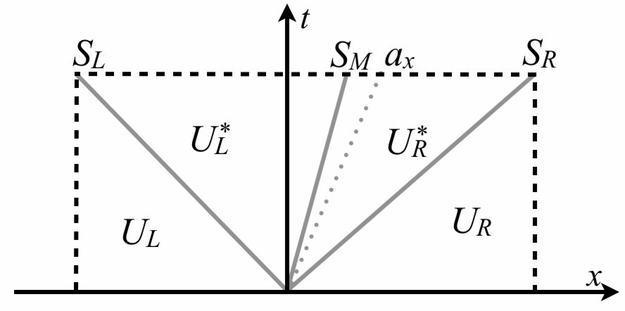
Figure 1: This figure shows the wave-structure of HLLC Riemann solver. Namely, HLLC solver resolves all three HD waves: left, right, and middle wave also known as contact discontinuity waves. The left and right wave can be either shock or rarefaction wave, or both. This solver approximates the structure of the two intermediate states, between $S_{L}$ and $S_{M}$, and $S_{M}$ and $S_{R}$, by a constant state.

A typical wave-structure of HLLC solver is shown in Fig. 1. The velocity of left, right and middle waves are $S_{L}$, $S_{R}$ and $S_{M}$ respectively, and the constant states sandwiched between these waves are $U^{\prime*}_{L}$ and $U^{\prime*}_{R}$ respectively. The HLLC-flux at the interface moving with velocity $a^{\prime}_{x}$ is

$${\cal G}^{\prime HLLC}=\left\{\begin{array}[]{ll}{\cal F}^{\prime}_{L}-a^{\prime}_{x}{\cal U}^{\prime}_{L}&a^{\prime}_{x}<S_{L},\\ {\cal F}^{\prime}_{L}+S_{L}({\cal U}^{\prime*}_{L}-{\cal U}^{\prime}_{L})-a^{\prime}_{x}{\cal U}^{\prime*}_{L}&S_{L}\leq a^{\prime}_{x}\leq S_{M},\\ {\cal F}^{\prime}_{R}+S_{R}({\cal U}^{\prime*}_{R}-{\cal U}^{\prime}_{R})-a^{\prime}_{x}{\cal U}^{\prime*}_{R}&S_{M}\leq a^{\prime}_{x}\leq S_{R},\\ {\cal F}^{\prime}_{R}-a^{\prime}_{x}{\cal U}^{\prime}_{R}&S_{R}\leq a^{\prime}_{x},\end{array}\right.$$ (33)

where ${\cal F}^{\prime}_{L}={\cal F}({\cal U}^{\prime}_{L})$ and ${\cal F}^{\prime}_{R}={\cal F}({\cal U}^{\prime}_{R})$. The intermediate states are defined by

$${\cal U}^{\prime*}_{K}=\rho_{K}\left(\frac{S_{K}-v^{\prime}_{xK}}{S_{K}-S_{M}}\right)\left[\begin{array}[]{c}1\\ S_{M}\\ v^{\prime}_{yK}\\ v^{\prime}_{zK}\\ \frac{E_{K}}{\rho_{K}}+(S_{M}-v^{\prime}_{xK})\left(S_{M}+\frac{p_{K}}{\rho_{K}(S_{K}-v^{\prime}_{xK})}\right)\end{array}\right],$$ (34)

for $K=L$ and $K=R$. Finally, estimates of wave speeds are $S_{L}=\min(v^{\prime}_{xL},v^{\prime}_{xR})-c_{\rm s}$ and $S_{R}=\max(v^{\prime}_{xL},v^{\prime}_{xR})+c_{\rm s}$, where $c_{\rm s}=\max(c_{{\rm s}L},c_{{\rm s}R})$. Other wave-speed estimates, such as those based on Roe-averages, can be used as well. Finally, the speed of the middle wave and the pressure in the $\star$-states is given by the following formulae

$$S_{M}=\frac{p_{R}-p_{L}+\rho v^{\prime}_{xL}(S_{L}-v^{\prime}_{xL})-\rho v^{\prime}_{xR}(S_{R}-v^{\prime}_{xR})}{\rho_{L}(S_{L}-v^{\prime}_{xL})-\rho_{R}(S_{R}-v^{\prime}_{xR})},$$ (35)

$$p^{\star}=\frac{(S_{R}-v_{xR})\rho_{R}p_{L}-(S_{L}-v_{xL})\rho_{L}p_{R}+\rho_{L}\rho_{R}(S_{R}-v_{xR})(S_{L}-v_{xL})(v_{xR}-v_{xL})}{(S_{R}-u_{R})\rho_{R}-(S_{L}-u_{L})\rho_{L}},$$ (36)

with $v^{\star}_{xL}=v^{\star}_{xR}=S_{M}$ and $p^{\star}_{L}=p^{\star}_{R}=p^{\star}$.

4.2 Ideal MHD

Our meshless conservative equations can also be applied to the equations of ideal MHD. In particular, we can rewrite MHD equations in the conservative form with the following conservative variables, fluxes and source terms

$${\cal U}=\left(\begin{array}[]{c}\rho\\ e_{\rm tot}\\ \rho{\bf v}\\ {\bf B}\\ \end{array}\right),\quad{\cal F}=\left(\begin{array}[]{c}\rho{\bf v}\\ (e_{\rm tot}+P_{T}){\bf v}-({\bf v}\cdot{\bf B}){\bf B}\\ \rho{\bf v}\otimes{\bf v}+P_{T}{\bf I}-{\bf B}\otimes{\bf B}\\ {\bf v}\otimes{\bf B}-{\bf B}\otimes{\bf v}\\ \end{array}\right),\quad{\cal S}=\left(\begin{array}[]{c}0\\ 0\\ {\bf 0}\\ {\bf 0}\\ \end{array}\right),$$ (37)

here $P_{T}=p+{\bf B}^{2}/2$ is sum of the thermal and magnetic pressures. The biggest difficulty in solving these equations is to maintain $\nabla\cdot{\bf B}=0$ constraint. While there are several ways to satisfy this constraint in finite-difference methods, it is not clear how this can be done in meshless schemes. In SPH, Rosswog & Price (2007) were able to circumvent this problem via use of the Euler potentials, $\alpha$ and $\beta$, which in smooth flows are advected with the flow, and are used to compute magnetic field ${\bf B}=\nabla\alpha\times\nabla\beta$. While mathematically this guarantees zero-divergence, in practice, however, the divergence is non-zero because of non-commuting nature of SPH cross-derivatives. This is also holds for the vector potential, ${\bf A}$, which may explain unstable behaviour of SPMHD equations with vector potential (Price, 2010). While SPH equations appear to be stable in the Euler potential formulation, they are unable to model topologically non-trivial field configurations (Brandenburg, 2010), and therefore are not suited to simulate complex magnetic field evolution, such as winding of magnetic field lines and magneto-rotational instability. Motivated by this, and by the fact that the existing MHD Riemann solvers use magnetic field as a primary quantity, we chose to evolve ${\bf B}$ instead, and apply one of the divergence cleaning methods known to work in Godunov finite-difference MHD schemes.

In their paper, Powell et al. (1999) showed that a self-consistent MHD equations must include source terms proportional to $\nabla\cdot{\bf B}$ to insure stability and Galilean invariance

$${\cal S}=-\nabla\cdot{\bf B}\left(\begin{array}[]{c}0\\ {\bf v}\cdot{\bf B}\\ {\bf B}\\ {\bf v}\\ \end{array}\right).$$ (38)

While this formulation both removes the instabilities associated with non-zero divergence and tends to keep the divergence at the truncation level, the divergence can still grow in certain situations. To avoid this, we also include a Galilean invariant form of the hyperbolic-parabolic divergence cleaning method due to Dedner et al. (2002), which results in the following system

$${\cal U}=\left(\begin{array}[]{c}\rho\\ e_{\rm tot}\\ \rho{\bf v}\\ {\bf B}\\ \rho\psi\\ \end{array}\right),\quad{\cal F}=\left(\begin{array}[]{c}\rho{\bf v}\\ (e_{\rm tot}+P_{T}){\bf v}-({\bf v}\cdot{\bf B}){\bf B}\\ \rho{\bf v}\otimes{\bf v}+P_{T}{\bf I}-{\bf B}\otimes{\bf B}\\ {\bf v}\otimes{\bf B}-{\bf B}\otimes{\bf v}\\ \rho\psi{\bf v}\\ \end{array}\right),\quad{\cal S}=\left(\begin{array}[]{l}\qquad 0\\ -(\nabla\cdot{\bf B}){\bf v}\cdot{\bf B}-{\bf B}\cdot\nabla\psi\\ -(\nabla\cdot{\bf B})\,{\bf B}\\ -(\nabla\cdot{\bf B})\,{\bf v}-\nabla\psi\\ -(\nabla\cdot{\bf B})c_{h}^{2}\rho-\psi\rho/\tau\\ \end{array}\right).$$ (39)

Here, $c_{h}$ and $\tau$ is the speed and the damping timescale of the divergence wave, also known as 8-wave, respectively. Usually, $c_{h}$ is set to be highest characteristic speed, i.e. that of the fast magnetosonic wave, $\tau=L/(c_{\bf r}c_{h})$, where $L$ is an effective size of the particle defined in §3.3, and $c_{\bf r}$ is a constant, which, following Mignone & Tzeferacos (2010), we set $c_{\bf r}=0.03$.

In their paper, Dedner et al. (2002) also presented a method to generalise an arbitrary 1D MHD Riemann solver to include an additional scalar field $\psi$ which transports the divergence away form the source and damps it. In general, the left and right reconstructed states in coordinate system ${\cal A}$ (see §4.1) have discontinuous $B^{\prime}_{x}$–the magnetic field component normal to the interface. The 1D Riemann solvers, however, require this field to be continuous, and this can be computed with the following equations

$$\bar{B}^{\prime}_{x}=\frac{1}{2}(B^{\prime}_{xL}+B^{\prime}_{xR})-\frac{1}{2c_{h,ij}}(\psi_{R}-\psi_{L}),$$ (40)

$$\bar{\psi}=\frac{1}{2}(\psi_{L}+\psi_{R})-\frac{c_{h,ij}}{2}(B^{\prime}_{xR}-B^{\prime}_{xL}).$$ (41)

Here, $B^{\prime}_{xK}$ are the left ($K=L$) and right ($K=R$) reconstructed states for $B^{\prime}_{x}$ and $\psi$, and $c_{h,ij}=\max(c_{h,i},c_{h,j})$. These interface values of $\bar{B}^{\prime}_{x}$ and $\bar{\psi}$ are used to compute $\nabla\cdot{\bf B}$ and $\nabla\psi$ respectively, which are required for the source terms in Eq. 39,

$$V_{i}(\nabla\cdot{\bf B})_{i}=-\sum_{j}\bar{B}^{\prime}_{x}|{\bf n}_{ij}|,$$ (42)

$$V_{i}(\nabla\psi)_{i}=-\sum_{j}\bar{\psi}\,{\bf n}_{ij}.$$ (43)

In Appendix B, we provide standard formulae to compute HLL and HLLD fluxes for the 1D MHD Riemann problem, which take $\bar{B}^{\prime}_{x}$ as the continuous normal component of the magnetic field. Finally, the advection flux for the scalar $\rho\psi$ is

$$F_{\psi}=F_{\rho}\times\left\{\begin{array}[]{cc}\psi_{L},&{\rm if}\,\,F_{\rho}>0,\\ \psi_{R},&{\rm otherwise},\end{array}\right.$$ (44)

where, $F_{\rho}$ is a mass flux given by the Riemann solver. This completes the description of our meshless MHD scheme.

5 Scheme validation

The weighted particle scheme is validated on several standard problems for ideal hydrodynamics and MHD problems, which are usually used to test hydrodynamic and MHD schemes (e.g. Tóth, 2000, Stone et al., 2008. In all simulations what follows, we use $N_{\rm ngb}=19$ and $32$ in Eq. 15 for 2D and 3D simulations respectively. This choice is motivated by the analogy with finite-difference schemes. In one dimension, the number of the neighbouring cells that a given cell interacts with depends on the order of the numerical scheme, and is usually two for the second order scheme. In SPH, two to four neighbouring particles are usually used in one-dimensional simulations. If this number is scaled to three dimensions, and taking into account that a kernel has spherical shape, the estimated number of neighbours are 16 and 32 for 2D and 3D respectively. The MHD simulations in 2D appear noisy with $N_{\rm ngb}=16$, which motivated us to use larger $N_{\rm ngb}$. In principle, large $N_{\rm ngb}$ can be used, should this be necessary, but this will decrease the resolution due to larger smoothing length.

5.1 Shock tubes

5.1.1 Brio-Wu shock tube

This problem was introduced by Brio & Wu (1988) to test the ability of an MHD scheme to accurately model shock waves, contact discontinuities and compound structures of MHD. Here, the problem is solved in a periodic 2D domain of size $[0,4]\times[0,0.25]$ with randomly sampled $5\cdot 10^{4}$ particles; this results in an effective resolution of $895\times 56$. The particles are initially relaxed before the initial conditions are set. The left state, $x<2$, is set with the following values: $\rho_{L}=1$, $p_{L}=1$, $B_{yL}=1$. The right state has $\rho_{R}=0.125$, $p_{R}=0.1$ and $B_{yL}=-1$. Both states have zero initial velocities, $B_{z}=0$ and $B_{x}=0.75$. The problem is solved with an ideal gas equation of states and $\gamma=2$. Various profiles, e.g. density and pressure, at time $t=0.2$ are show in Fig. 2.

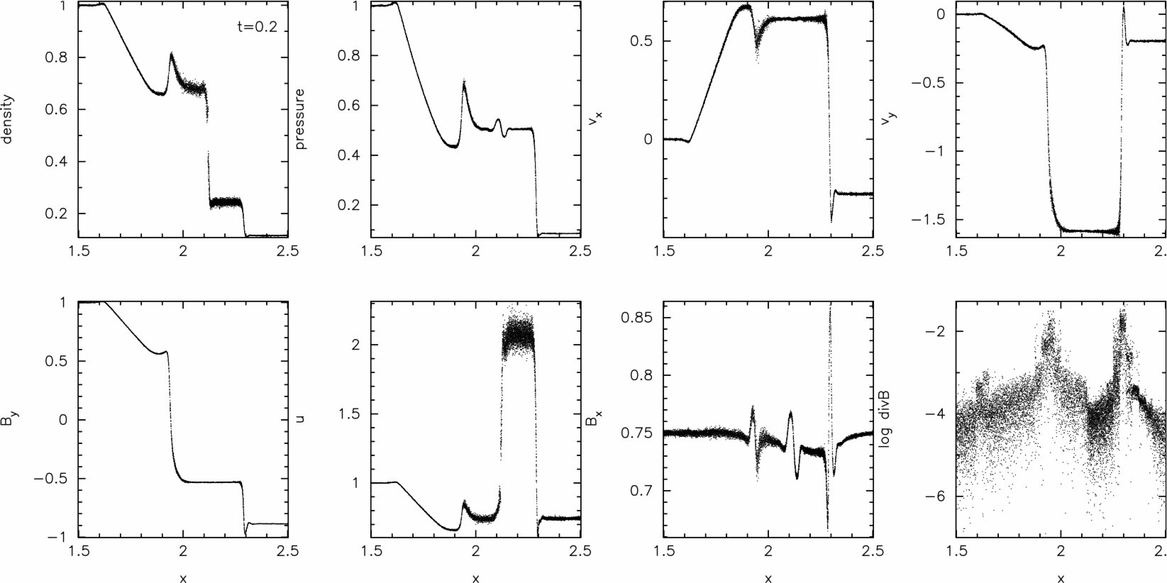
Figure 2: Solution to the Brio-Wu MHD shock tube problem at time $t=0.2$. The panels display (from left to right, top to bottom) density, gas pressure, $x$- and $y$- velocity profiles, $B_{y}$, thermal energy $u=P/\rho$, $B_{x}$ and the logarithm of ${\tt divB}=L\nabla\cdot{\bf B}/|{\bf B}|$, where $L$ is an effective size of a particle (§3.3).

The results are overall consistent with 1D Godunov-MHD scheme, namely jumps across the discontinuities and location of discontinuities. The two bottom right panels show the value of $B_{x}$ field and the ${\tt divB}=L\nabla\cdot{\bf B}/|{\bf B}|$ as a function of particle $x$-coordinate. The parallel magnetic field slightly deviates from its constant value, except near discontinuities where it exhibits jumps. The divergence, however, remains small, even across discontinuities. The existence of blip in pressure at location of contact discontinuity, $x\approx 2.1$, and shock waves, $x\approx 2.3$ has the same origin as in SPH: the particle distribution across a discontinuity is less regular in a sense that the approximation in Eq. (4 is not sufficient to provide accurate results. This is a known issue in Godunov SPH, and higher order approximations are able to reduce the amplitude of the blip (Inutsuka, 2002). Overall, the solution obtained by the meshless scheme is in a good agreement with high-resolution 1D Euleriean schemes.

5.1.2 Tóth shock tube

Another challenging shock tube problem was introduced by Tóth (2000). In this problem, two streams of magnetised gas supersonically collide with each other. Tóth (2000) showed that some MHD schemes with source terms proportional to $\nabla\cdot{\bf B}=0$ produce wrong jump conditions. This was challenged by Mignone & Tzeferacos (2010), who showed that if divergence is cleaned in hyperbolic-parabolic manner (Dedner et al., 2002), the jump conditions are correct even with the presence of the source terms. The problem is set in 2D periodic domain with size $[0,4]\times[0,0.25]$ with randomly distributed $5\cdot 10^{4}$ particles. After the particle distribution is relaxed, the following initial conditions are set. The left states has $\rho_{L}=1$, $p_{L}=20$, $v_{xL}=10$, and the right state has $\rho_{R}=1.0$, $p_{R}=1$, $v_{xR}=-10$. Both states have $B_{x}=B_{y}=5/\sqrt{4\pi}$. This problem is solved with an ideal gas equation of state and $\gamma=5/3$. The solution to this problem is shown in Fig. 3, which can be compared to solutions obtained by (Tóth, 2000) and Mignone & Tzeferacos (2010). Our meshless scheme is able to recover correct jump conditions and to maintain constant $B_{x}$ field within few percent accuracy, except across discontinuities. Furthermore, the divergence in this problem remains small.

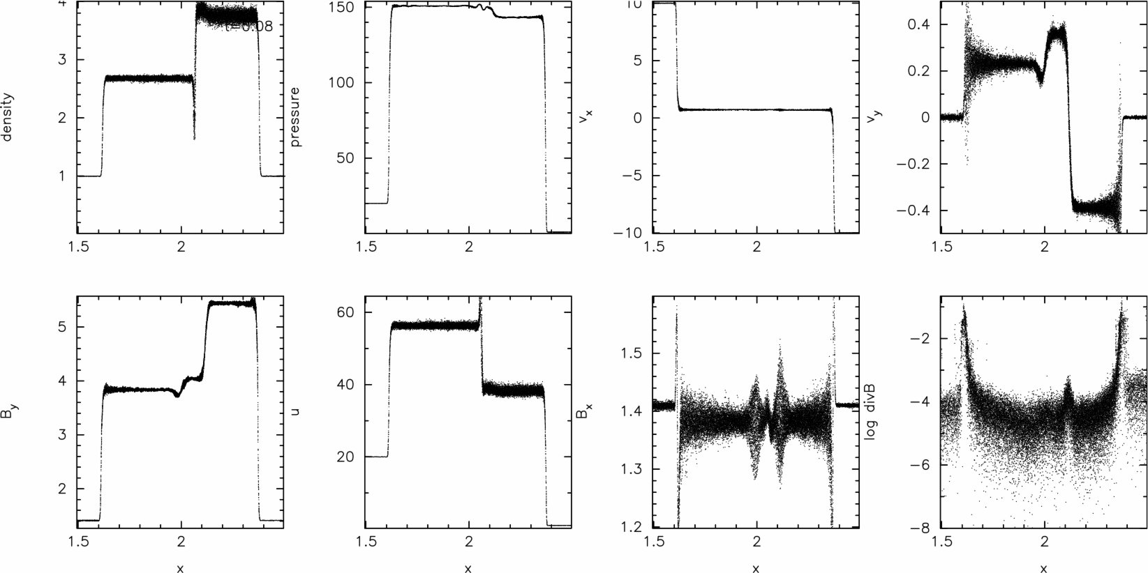
Figure 3: Solution to the Tóth MHD shock tube problem at time $t=0.2$. The panels display (from left to right, top to bottom) density, gas pressure, $x$- and $y$- velocity profiles, $B_{y}$, thermal energy $u=P/\rho$, $B_{x}$ and ${\tt divB}=L\nabla\cdot{\bf B}/|{\bf B}|$, where $L$ is an effective size of a particle.

5.2 Advection of a magnetic field loop

This problem tests the ability of the scheme to transport magnetic loop across computational domain. This problem is proven to be a stringent test for finite-difference schemes. The computational domain in this test is a cuboid with dimensions $[0,2]\times[0,1]\times[0,0.5]$ which is initially filled with $128\times 64\times 32$ particles on cubic lattice to assure zero noise. The fluid state is set to $\rho=2$ inside the loop and $\rho=1$ outside the loop, $p=1$, ${\bf v}=(2,1,0.5)$ and ${\bf B}=(f(R)y,-f(R)x,0)$, where $R=\sqrt{x^{2}+y^{2}}$ and

$$f(R)=\left\{\begin{array}[]{cl}B_{0}/R&0<R<R_{0},\\ 0,&{\rm otherwise}.\end{array}\right.$$ (45)

Here, $R_{0}=0.3$ is a radius of the loop, $B_{0}=10^{-3}$ is the initial magnetic field strength that results in $2\beta=P_{\rm gas}/P_{\rm mag}=10^{6}$. With such high $\beta$ magnetic field does not play dynamical role and should be transported as a passive scalar. Periodic boundary conditions are used in this test, and the ideal gas equation of state with $\gamma=5/3$.

In Fig. 4 we shows magnetic field structure at the $t=0$ and $t=10$, which corresponds to ten crossings of the computational domain, and in Fig. 5 we show the magnetic energy as a function of time. This figures demonstrate the ability of the meshless scheme to advect magnetic loop quite well. Furthermore, the decay of the magnetic energy is at least as slow as resulted from high-order Godunov MHD schemes. This is certainly expected in light of semi-Lagrangian nature of the scheme. One may however expect that the energy should not decay at all since the magnetic field is transported as a passive scalar. Indeed, Fig. 6 demonstrates that the scheme is able to transport mass, and therefore passive scalar, without any diffusion. The difference with magnetic field stems from the different nature of equation that transport mass, or advect passive scalar, and the induction equation as implemented in the scheme. In fact, the decay is caused solely by the diffusion of magnetic field due to divergence cleaning equations, i.e. Eq. (40 and Eq. 41. The fluxes resulting from HLLD Riemann solver are in fact zero since both particles and the frame move with the same velocity. The divergence of the magnetic field, even though is zero analytically, is not necessary zero in the discretisation set by Eq. 40 andEq. 42, and this produces evolution of magnetic field due to non zero value of $\nabla\psi$ in the source terms of Eq. 39. Among all discretisations studied by Tóth (2000), this is the special one because of its use in the discretisation of Maxwell stress term to obtain Lorentz force. If the $\nabla\cdot{\bf B}=0$ in this discretisation, no force parallel to magnetic field exists, and therefore the source terms proportional to this divergence vanishes. Incidentally, this is the discretisation of divergence that is enforced to zero in constrained transport (CT) formalism (Evans & Hawley, 1988). More importantly, the maintenance of zero divergence in other discretisations, such as cell-centred, does not guarantee vanishing divergence in CT-discretisation, but this will probably be small thus giving minimal damage to the solution.

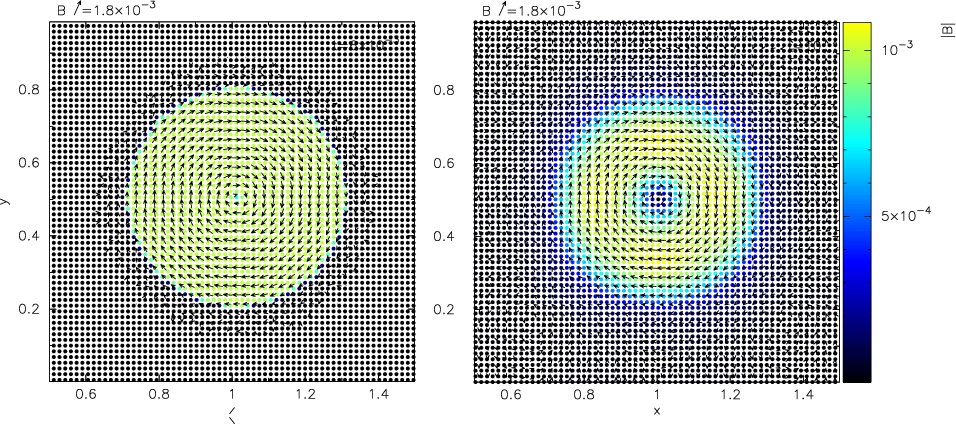
Figure 4: Amplitude (colours) and direction (vectors) of magnetic field at the beginning (left panel, $t=0$) and at the end (right panel, $t=10$) of the simulation. The magnetic field distribution is show in the $XY$-plane passing through $z=0.25$. In the right panel, the strength of magnetic field in the centre is close to zero due to numerical resistivity, which is consistent with finite-difference calculations.

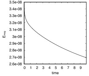
Figure 5: This figure demonstrates decay of magnetic energy during advection of magnetic field loop. The magnetic energy decay is due to numerical resistivity introduced by divergence cleaning procedure, and not through the solution of an MHD Riemann problem.

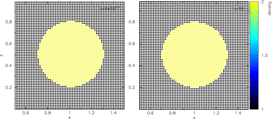
Figure 6: This figure shows that our scheme is able to transport mass, and therefore passive scalars, without any numerical diffusion in a constant velocity field. The right and left panels show plots of the density field in the $XY$-plan passing through $z=0.25$, at the beginning and the end of the simulation respectively.

5.3 Blob test

An interesting and challenging problem to test particle hydrodynamic schemes has been proposed by Agertz et al. (2007). This problem demonstrates the destructive property of the Kelvin-Helmholtz instability (KHI) in three-dimensional simulations. The setup consist of a dense cloud with $\rho_{\rm cl}=10$ moving supersonically through a less dense ambient fluid with $\rho_{\rm amb}=1$. Initially, the cloud is at rest and in the pressure equilibrium with the ambient fluid, at $p_{\rm amb}=1$. The velocity of the ambient medium is ${\bf v}=(2.7c_{\rm s,amb},0,0)$, where $c_{\rm s,amb}$ is its sound speed. The cloud radius is $R_{\rm cl}=0.1$, and an ideal gas equation of state is used with $\gamma=5/3$. The initial magnetic field is set to zero, and it will stay so throughout the simulation. This problem is set in a periodic domain with dimensions $[0,3]\times[0,1]\times[0,1]$, in which $7\cdot 10^{5}$ particles are sampled in the strip $|y-0.5|<1.1R_{\rm cl}$ and $3\cdot 10^{5}$ outside. This setup permits to resolve cloud and the impacting ambient fluid with high resolution ($h\sim 0.01$) for a total of $10^{6}$ particles. The particles are sampled from a three-dimensional Sobol quasi-random sequence (Press et al., 1992). To remove the initial noise, this initial particle distribution is relaxed before the initial values for the density field, pressure and velocity are set.

Following Agertz et al. (2007), the Kelvin-Helmholtz timescale is defined $T_{\rm KH}=1.6\tau_{\rm cr}$, where $\tau_{\rm cr}=2R_{\rm cl}\sqrt{\rho_{\rm cl}/\rho_{\rm amb}}/v_{\rm amb}$. For parameters used in this simulations, this gives $T_{\rm KH}\approx 0.3$. The snapshots of the density distribution in plane $z=0.5$ at $t=0.5,1.0,1.5$ and $2.5\,T_{\rm KH}$ are shown in Fig. 7. These are in an excellent agreement with those presented in Agertz et al. (2007). The time dependence of cloud mass is shown in Fig. 8, where a particle is considered to be part of a cloud if $\rho>0.64\rho_{\rm cl}$ and $T<0.9T_{\rm amb}$. In agreement with finite-difference methods, the cloud lost nearly 90% of its mass within $2\,T_{\rm KH}$.

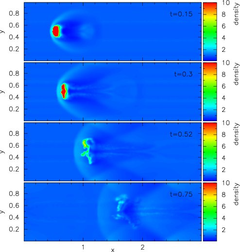
Figure 7: Density field plot in $XY$-plane passing through $z=0.5$. The panels show density profile at time $0.5$, $1.0$, $1.5$ and $2.5$ $T_{\rm KH}$, where $T_{\rm KH}\approx 0.3$. At $t=0.5T_{\rm KH}$ (top panel), the cloud shape is distorted by RAM pressure. At $t=T_{\rm KH}$ (second panel from the top), the KHI instability deforms the shape of the cloud further. The cloud destruction begins at $t=1.5T_{\rm KH}$, and by $t=2.5T_{\rm KH}$ the cloud lost more than 90% of its mass.

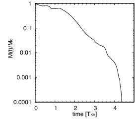
Figure 8: This plot show cloud mass as a function of time. In agreement with finite-difference scheme the cloud looses most of its mass at $t\approx 2$ $T_{\rm KH}$, and is completely destroyed at $t\gtrsim 3T_{\rm KH}$.

5.4 Spherical blast-wave

The problem is initiated with an overpressured central region in a uniform density and magnetic field. The computational domain is a unit square filled with fluid with $\rho=1$. Within $R<R_{0}=0.1$, the pressure is set to $10$, whereas outside $p=0.1$. In magnetised case, there is also a uniform magnetic field ${\bf B}=(1/\sqrt{2},1/\sqrt{2},0)$. The equation of state is that of an ideal gas with $\gamma=5/3$. The particles are sampled in a periodic box $[0,1]\times[0,1.5]$, such that $5\cdot 10^{4}$ particles are randomly sampled in three nested rectangles: $[0,1]\times[0.1,5]$, $[0.25,0.75]\times[0.375,1.125]$ and $[0.375,0.625]\times[0.5625,0.9375]$. Before the initial conditions are set, the particles are relaxed into a regular distribution to reduce start-up noise. In figures 9 and 10 we show density plots for non-magnetised and magnetised cases respectively. Of particular interest here is the ability of the particle weighted method to resolve Richtmyer-Meshkov instability, shown in right panel of Fig. 9. In the magnetised case, however, the presence of strong magnetic field inhibits development of this instability (the right panel of Fig. 10).

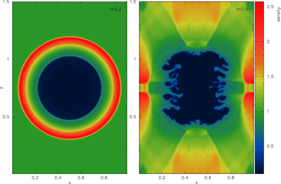
Figure 9: This figure show the density at $t=0.2$ and $t=1.5$ for non-magnetised spherical blast wave problem. The location of the shock front is in agreement with high-resolution conservative numerical schemes (Stone et al., 2008). Right panel show dense fingers in rarefied media which are formed by Richtmyer-Meshkov instability. This demonstrates that our scheme is able to capture important fluid instabilities without any fine-tuning.

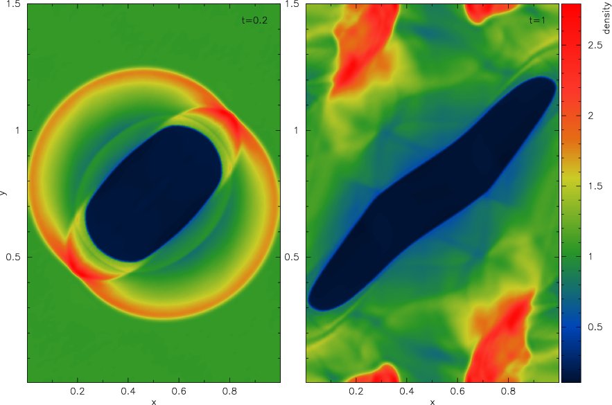
Figure 10: This figure show the density at $t=0.2$ and $t=1$ for magnetised spherical blast wave problem. The initial magnetic field in this problem has angle of $\pi/4$ with $x$-axis. Since the shock moves more easily along the magnetic field lines, this explains the elongated shape of the shock-front, which contrasts with hydrodynamical case. As in hydrodynamical test, here the location of shock from is in excellent agreements with conservative Eulerian MHD schemes (Stone et al., 2008). The right panel, shows further evolution of the black wave, after shock reached the rarefied medium. In contrast to the hydrodynamical case, magnetic field inhibits development of Richtmyer-Meshkov instability.

5.5 Orszag-Tang vortex

The Orszag-Tang vortex (Orszag & Tang, 1979) is a standard test problem that is used to validate many numerical MHD schemes. The setup involves periodic domain of size $[0,1]\times[0,1]$ with an adiabatic equation of state with $\gamma=5/3$. The initial density and pressure are set in all computational domain to $25/(36\pi)$ and $5/(12\pi)$ respectively. The velocity ${\bf v}=(-\sin(2\pi y),+\sin(2\pi x),0)$ and magnetic field ${\bf B}=(-B_{0}\sin(2\pi y),B_{0}\sin(4\pi x),0.0)$, where $B_{0}=1/\sqrt{4\pi}$. The second simulation involves the same initial conditions, with the exception that the problem is solved a boosted frame, with the initial velocity ${\bf v}={\bf v}_{\rm rest}+{\bf v}_{\rm boost}$, where ${\bf v}_{\rm boost}=(10,10,10)$. The simulation is solved with $10^{5}$ particles, where first $5\cdot 10^{4}$ where randomly sampled within the square $[0,1]\times[0,1]$ and the second $5\cdot 10^{4}$ in the square of half size, $[0.25,0.75]\times[0.25,0.75]$. This permitted to achieve high resolution in the central region of the problem. The initial conditions were set, as soon as distribution was relaxed.

In the Fig. 11 we show density at $t=0.5$ for both rest-frame and boost-frame initial conditions, and in Fig. 12 we show particle distribution. As expected, there are no discernible differences, and both simulations resolve discontinuities well. Furthermore, due to Lagrangian nature of the method, the particle number density correlates with the mass density. It is worth pointing out that in this particular simulation, the particle distribution appears to remain regular even in the vicinity of the shocks. The Fig. 13 show 1D pressure profile at $y=0.3125$ (top) and $y=0.427$ (bottom) for both boosted and rest-frame simulations. The agreement with finite-difference scheme is excellent, ac can be compared to published results (e.g. Tóth, 2000, Rosswog & Price, 2007, Stone et al., 2008). In contrast to shock-tube problems, no pressure blips are visible here.

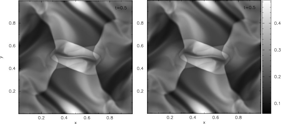
Figure 11: Density distribution of Orszag-Tang vortex at $t=0.5$. The left and right panels show the result of the simulation in the rest and boosted frame respectively. We point out that even at low resolution our scheme is able to resolve the fine structure in the bottom left quadrant; in this quadrant, the effective resolution is $128\times 128$, compared to $256\times 256$ in the centre.

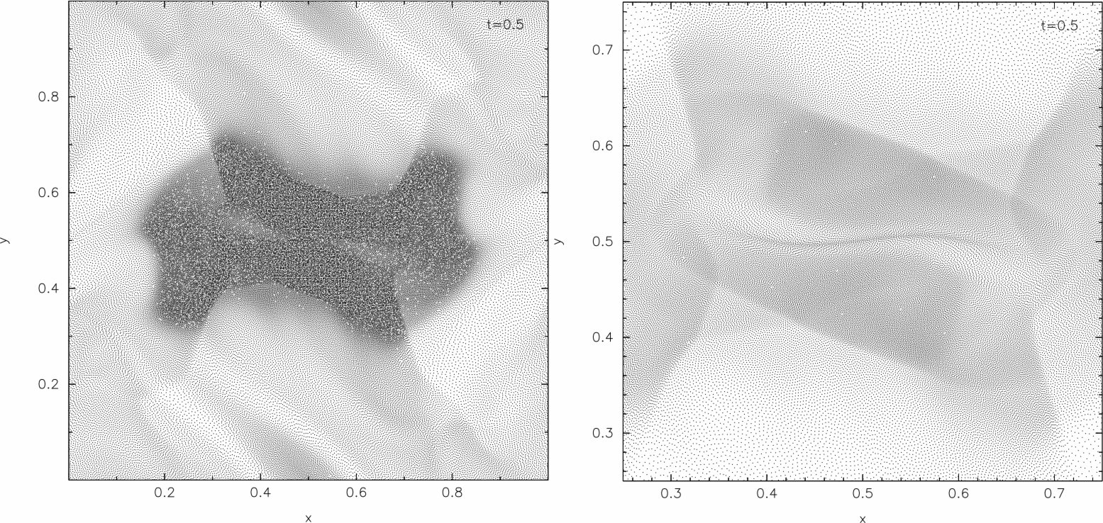
Figure 12: Particle distribution of Orszag-Tang vortex at $t=0.5$. The left and right panels show the particle distribution in all domain and in the central region respectively. Due to Lagrangian nature of the simulation, the particle distribution correlated with that of the density. We would like to note that even across the shocks, the particle distribution remains remarkably regular without any observable signs of clumping.

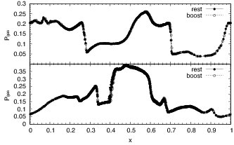
Figure 13: Pressure distribution of Orszag-Tang vortex at $t=0.5$ and $y=0.3125$ (top) and $y=0.427$ (bottom). This can be compare to the results of other finite-difference or meshless MHD schemes (e.g. Rosswog & Price, 2007; Stone et al., 2008). In particular, our scheme has little noise in pressure, and the shock waves are resolve within few particles, without observable oscillatory behaviour in post-shock regions.

5.6 MHD rotor

The rotor problem, introduced by Balsara & Spicer (1999) to test propagation of strong torsional Alfvén waves, is also considered as one of the standard candles to validate numerical MHD schemes. Here, the computational domain is a unit square, $[0,1]\times[0,1]$. The initial pressure and magnetic field are uniform with values $p=1$ and ${\bf B}=(5/\sqrt{4\pi},0,0)$. Inside $R<R_{0}=0.1$ there is a dense uniformly rotating disk with $\rho=10$ and ${\bf v}=(-2y/R_{0},+2x/R_{0},0)$, where $R=\sqrt{x^{2}+y^{2}}$. The ring $R_{0}<R<R_{1}=0.115$ is occupied by a transition region with $\rho=1+9f(R)$ and ${\bf v}=(-2yf(R)/R,+2xf(R)/R,0)$, where

$$f(R)=\left\{\begin{array}[]{cl}1&R<R_{0},\\ \frac{R_{1}-R}{R_{1}-R_{0}}&R_{0}\leq R<R_{1}\\ 0&R_{1}<R.\end{array}\right.$$ (46)

Outside $R>R_{1}$, the velocity is set to zero and $\rho=1$. This problem uses an ideal gas equation of state with $\gamma=1.4$. The particles are distributed in the same way as in strong blast wave problem (§5.4). The problem is solved in both rest and boosted frames, with $v_{\rm boost}=(5/0.15,5/0.15,5/0.15)$. The plots of density, gas and magnetic pressure, and mach number are shown in Fig. 14. The 1D slices of magnetic field at $x=0.5$ and $y=0.5$ are show in Fig. 15 to facilitate comparison to Eulerian MHD schemes.

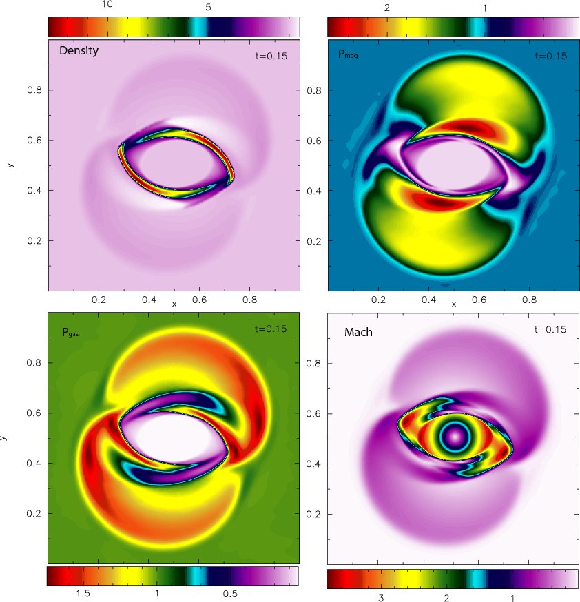
Figure 14: Density (top left), gas pressure (bottom left), magnetic pressure (top right) and Mach number (bottom right) plots for MHD rotor problem at $t=0.15$. The Mach number panel plots Mach number using rest-frame velocities, that is first subtracting the boost velocity and afterwards computing mach number. The result of the rest frame simulation have little difference, and therefore not presented here. The colour coding is chosen to facilitate the comparison with published results produced by FLASH3 code for this problem (Fryxell et al., 2000, Sect 21.2.3 in FLASH 3 user guide manual http://flash.uchicago.edu/website/codesupport/flash3_ug_beta).

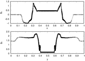
Figure 15: Distribution of $B_{y}$ in $y=0.5$ slice (top pannel) and $B_{x}$ in $x=0.5$ slice (bottom) for MHD rotor problem at $t=0.15$. This plots can be readily compared to Fig.26 of (Stone et al., 2008). The agreement is rather good everywhere, except for $B_{y}$ near $x\approx 0.34$ and $x\approx 0.66$, where the meshless scheme appears to diffuse the discontinuity in magnetic field.

5.7 Magneto-rotational instability

Magneto-rotational instability, or MRI for short, is a powerful local instability in weakly magnetised disks that plays an important role in astrophysics (Balbus & Hawley, 1991, 1998). The ability of the scheme to model this instability is crucial for simulation of magnetised accretion disks, or any other simulation where non-trivial MHD effects are expected to appear. Below we conduct two simulations that test the ability of the meshless MHD scheme to faithfully model MRI.

5.7.1 2D axisymmetric shearing box

The first simulation is solved in a local 2D axisymmetric shearing sheet with the initial conditions exactly the same as in the fiducial model of Guan & Gammie (2008). To repeat, the unit box has a size $[0,1]\times[0,1]$ with an initially uniform density fluid with unit density, $\rho_{0}=1$, embedded in a vertical magnetic field $B_{z}=B_{0}\sin(2\pi x/\lambda_{\rm MRI})$, where $\lambda_{\rm MRI}=2\pi\sqrt{16/15}v_{\rm A}/\Omega$ is the fastest growing MRI wavelength, $v_{\rm A}=B_{0}/\sqrt{\rho_{0}}$ is Alfvén speed, and $\Omega$ is angular velocity which is set to unity throughout the simulation. The magnetic field strength $B_{0}=\sqrt{2p_{0}/\beta_{0}}$, where $\beta_{0}=1348$ in order to excite $m=4$ MRI mode. The instability is seeded by random velocity perturbation $\delta v=0.01c_{s}$. Isothermal gas equation of state is used, $p=c_{s}^{2}\rho$, with $c_{s}=1$ in all domain at all times. The boundary conditions are periodic in $z$-direction, shear-periodic $x$-direction, i.e.

$$f(x,z)=f(x+n_{x}L_{x},z+n_{z}L_{z}),$$ (47)

$$v_{y}(x,z)=v_{y}(x+n_{x}L_{x},z+n_{z}L_{z})+n_{x}q\Omega L_{x}.$$ (48)

Here, $q=-1/2d\ln\Omega/d\ln R$ which is equal to $3/2$ for a Keplerian disk, and $n_{x}$ and $n_{y}$ are arbitrary integer numbers. In this shearing box model, the momentum equation have the following form

$$\partial_{t}(\rho{\bf v})=-\nabla\cdot(\rho{\bf v}\otimes{\bf v}+P_{T}{\cal I}-{\bf B}\otimes{\bf B})-2\Omega\times(\rho{\bf v})+2\rho q\Omega^{2}x\hat{x},$$ (49)

where $P_{T}=p+B^{2}/2$ is the sum of the thermal and the magnetic pressure, the second and third terms on the right hand side are Coriolis and centrifugal forces respectively.

This problem is solved in a periodic domain, with $128\times 128$ and $256\times 256$ particles initially distributed on Cartesian grid. The toroidal, $B_{y}$, component of magnetic field is show in Fig. 16 at $t=5$, $10$, $15$ and $20$. The $m=4$ MRI mode is clearly seen at $t=10$, and the bottom right panel demonstrates the break up of the laminar flow into turbulent. Fig. 17 shows both the toroidal magnetic field (left panel) and ${\tt divB}$ (right panel) at $t=40$. The aim is to demonstrate that even in turbulent flows, the scheme is able to keep the divergence small. Time dependence of magnetic field energy and Maxwell-stresses is show in Fig. 18. The initial growth can be fit with $E_{\rm mag}/U\propto\exp(0.75t)$, and is in excellent agreement with Fig.4 and Fig.11 of Guan & Gammie (2008). The decay at late times differs, which is an expected result, since this depends on the details of numerical dissipation, which differs among MHD schemes.

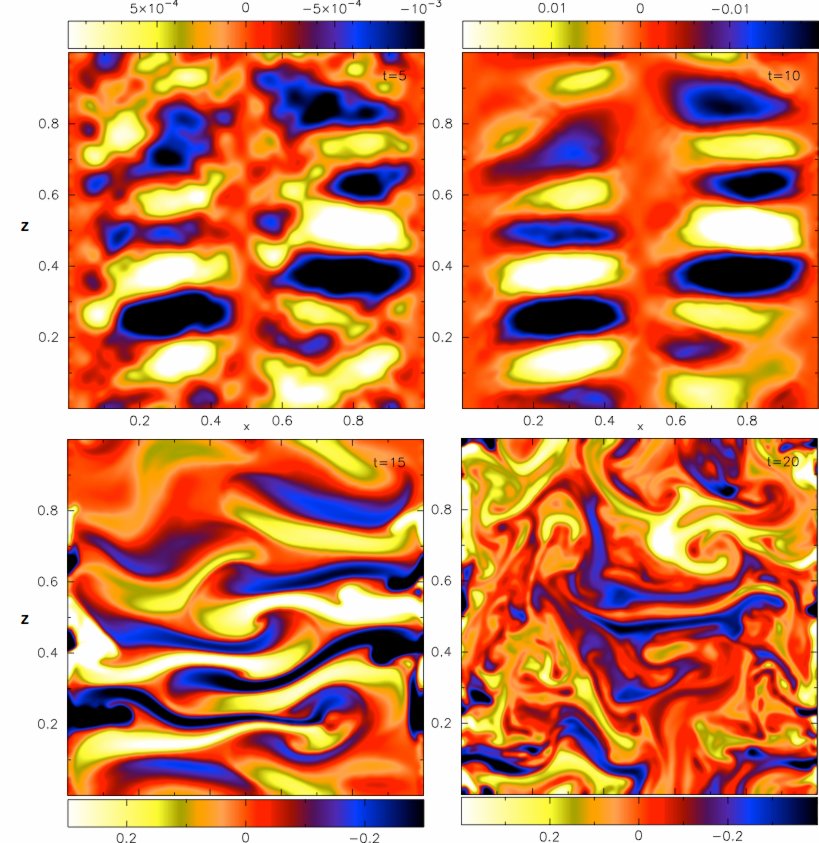
Figure 16: Toroidal, $B_{y}$, magnetic field at $t=5$ (top left) , $t=10$ (top right), $t=15$ (bottom left) and $t=20$ (bottom right) for 2D shearing box simulation at $256\times 256$ resolution. At $t=10$ panel, the $m=4$ MRI mode can be seen, in an excellent agreement with the MRI theory, and at $t=20$ the flow becomes turbulent in agreement with finite-difference MHD schemes.

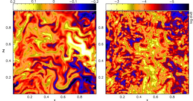
Figure 17: The figure show toroidal magnetic field at late times, $t=40$. The aim is to demonstrate the ability of the scheme to keep the divergence low even in turbulent flows.

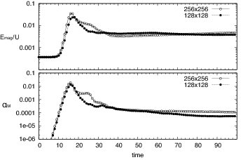
Figure 18: Time dependence of volume averaged magnetic energy and Maxwell stresses as a+ function of time. This figure can be readily compared to Fig.4 and Fig.11 of Guan & Gammie (2008). The initial growth rate is in excellent agreement with their results. The subsequent turbulent evolution is different, however. This is a known result, since the turbulent evolution of the flow depends on the numerical scheme employed. Due to anti-dynamo theorem, the magnetic energy and Maxwell stresses decay in this 2D simulation.

5.7.2 3D Global disk simulation

The final test problem studies the evolution of a circular disk around a point-mass gravitational source. The aim is to test the particle scheme on realistic astrophysical simulation, and to determine its weak points. The problem is set up in a computational domain of size $[0,20]\times[0,20]\times[0,20]$ with a gravitational source of unit mass located at origin $(10,10,10)$. Following methods of Lodato & Rice (2004) and Alexander et al. (2008), a circular stratified disk is sampled with $10^{6}$ particle from its inner edge, $R_{\rm in}=1$, to its outer edge, $R_{\rm out}=4$, where $R=\sqrt{(x-10)^{2}+(y-10)^{2}}$ is the distance from the midplane of the disk to the gravitational source. The scale height of the disc is $H/R=0.1$, and only one scale height is sampled to avoid large density variations. Particles which fall within $R_{\rm min}=0.25R_{\rm in}$ and outside the computational domain are removed from the system. The particle distribution is regularised to minimise the start-up noise before the initial conditions are assigned. Since this problem uses open boundary conditions, we also imposed a lower and upper limit to the number of neighbours; specifically, we set $N_{\rm ngb,low}=8$ and $N_{\rm ngb,up}=128$ for the lower and upper limit respectively. We did this in order to prevent particles close to the boundaries to have either too few or too many neighbours. The lower limit, however, not been reached in our simulations.

The initial density in the disk is $\rho(R,z)=\rho_{\rm mid}\exp(-z^{2}/2H^{2})$, where $\rho_{\rm mid}=1$ is the density in the mid plane. The scale height is $H=c_{\rm snd}/v_{\rm circ}R$, where $v_{\rm circ}=\sqrt{1/R}$ and $c_{\rm snd}$ is sound speed of a particle. The latter is set to be constant in time, but has the following spatial variation $c_{\rm snd}=(H/R)v_{\rm circ}$. Pressure is set via isothermal equation of state, $p=c^{2}_{\rm snd}\rho$. The gravitational acceleration is split into horizontal and vertical component, to make sure that the above hydrostatic equilibrium is satisfied, namely $a_{\rm grav}=g(R)(x-10,y-10,z-10)$, where $g(R)=-1/R^{3}$. Two simulations where run with above initial conditions, one non-magnetised and one magnetised. In the latter case, initial constant vertical magnetic is set with $\beta=1348$ in the midplane, which have following $R$-variation, $B(R)=B_{0}\sin(2\pi(R-2))$, and the magnetic field outside the ring $2<R<3$ is set to zero. With this setup, the orbital period of an inner disk orbit is $2\pi$. The magnetic field is forced to be zero for $R<1.2$ and $R>6.5$.

Density structure of the disk in $XZ$-plan passing through the gravitational source is shown in Fig. 19 for $t=10$, $50$, $100$, $150$. The right panels on the figure show density distribution for non-magnetised case. As expected, the flow remains laminar throughout the simulation. However, at $t=100$, the inner edge of the disk is noticeably damaged due to particle loss through $R_{\rm min}$. This error, generated at the inner edge of the disk, slowly propagates outward, as can be seen by the further damage at $t=150$. This example demonstrates the importance of proper boundary conditions in meshless scheme. However, it is no clear how to define these. Nevertheless, the global structure of the disk remains consistent with the initial conditions and vertical hydrostatic equilibrium through the simulation.

In the left panel of the Fig. 19 we show density distribution of the magnetised case. In contrast to non-magnetised simulation, the laminar motion breaks into turbulence at $t\approx 100$. For earlier times, the laminar flow permits the magnetic field to grow to $\langle\beta^{-1}\rangle\approx 0.1$ as shown in the top panel of the Fig. 20. Of the particular interest here, is the value of the magnetic stresses, $\alpha_{\rm M}=-B_{r}B_{\theta}/P_{\rm gas}$, which determines the accretion rate in the disk. Time dependence of the volume average magnetic stress is shown in the bottom panel of the Fig. 20. The growth continues until $t\approx 100$, after which the flow become turbulent and the volume averaged magnetic stress remain roughly constant at $\langle\alpha_{\rm M}\rangle\approx 0.01$. In contrast to 2D axisymmetric shearing sheet simulation, neither magnetic energy nor magnetic stressed decay with time, implying the dynamo activity in the disk.

The density distribution in the mid plane of the disk is shown in Fig. 21. The left and right panels of the figure display non-magnetised and magnetised cases respectively, and the top and bottom panel show the profile at $t=100$ and $t=150$. The turbulent structure of the magnetised disk for $t>100$ is apparent through the existence of small scale structures in density, whereas the non-magnetised disk remains laminar, with the exception of small spiral waves which are caused by the error propagating from the inner disk boundary. The magnetic field structure is shown in Fig. 22 for $t=50$ (top panel) and $t=100$ (bottom panel). The left panel shows the amplitude of the toroidal magnetic field, $B_{\theta}$, and the value of Maxwell stresses, $B_{r}B_{\theta}$. At $t=50$, the structure begins to appear, but the magnetic field is weak to substantially influence the dynamical evolution of the disk. At $t=100$, however, the magnetic field is amplified to a large values via MRI mechanism, and has non-negligible effect on dynamics. Furthermore, the toroidal magnetic field exhibits reverse, cause by the shear, in agreement with the theoretical expectations.

Overall, the growth of magnetic field is consistent with published 2D and 3D shearing box simulation. Namely, the linear MRI regime is able to amplify magnetic field to $\langle\beta^{-1}\rangle\gtrsim 0.1$ until it breaks up into turbulence. Due to limited numerical resolution of this simulation, we were unable to resolve fastest growing MRI mode, which explains the slower than expected growth. Nevertheless, the magnetic stresses are roughly ten percent of magnetic energy, $\langle\alpha_{\rm M}\rangle\gtrsim 0.01$, and drive the accretion of the matter. This matter is accumulate at $R<1.25$ where magnetic field is set to zero at boundary condition, and explains dens blob of matter in the two lowest left panels of Fig. 19.

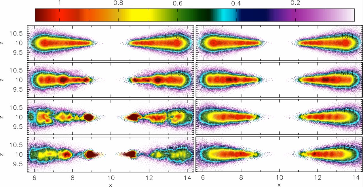
Figure 19: Density particle plot in $XZ$-plane passing through the centre $(10,10,10)$. The left and right panels shows snapshot from magnetised and non-magnetised cases respectively at $t=10$, $t=50$, $t=100$ and $t=150$ (from top to bottom). The magnetic start to play an important role at $t\gtrsim 50$ or after about 8 inner orbital periods

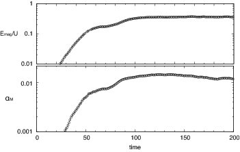
Figure 20: This figure shows the growth of the volume average magnetic field and Maxwelian stresses in the magnetised disk simulation. In agreement with the 2D shearing sheet simulation, the magnetic field and stresses reach its maximum after about 15 inner orbits (or 5.6 orbits at $R=2$. In contrast to 2D case, however, the magnetic field does not decay furthermore, but is maintained by dynamo action.

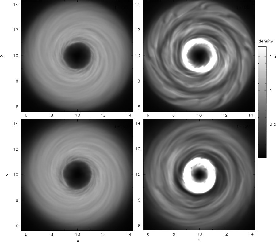
Figure 21: Density structure of the disk in $XY$-plan passing through the centre. The right and left panels show non-magnetised and magnetised cases respectively, at $t=100$ (top) and at $t=150$ (bottom). The density structure in magnetised disk at $t=50$ has same form as non-magnetised, and therefore is not shown here.

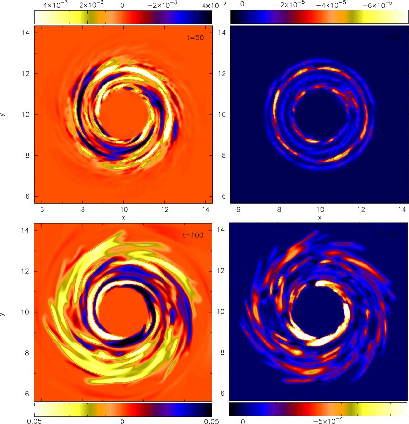
Figure 22: The left panel show the amplitude of toroidal field component, and the right panel the magnitude of Maxwell stress, $B_{r}B_{\theta}$ at $t=50$ (top) and $t=100$ (bottom). The field and the stresses at $t=150$ have the structures similar to those at $t=100$, and therefore are not shown here.

6 Discussion and Conclusions

This paper presents application of a new weighted particle scheme for conservation laws to the equations of ideal hydrodynamics and magnetohydrodynamics. This scheme has no free parameters which control the physics of the inter-particle interaction. There only free-parameter in our scheme is the average number of neighbours that a particle interacts with, and this depends only on the number of spatial dimensions. The interaction between particles is entirely described by the source terms and fluxes. The latter are given by the solution of the associated Riemann problem, which correctly treats dissipative processes and discontinuous solution without explicit use of artificial viscosity or resistivity. Due to use of Riemann solvers and reconstruction methods, our weighted particle method is expected to be more dissipative compared to pure Lagrangian SPH without any explicit diffusion terms. However, further quantitative comparison to SPH is required to verify this claim in realistic astrophysical problems, where dissipative processes, albeit locally, must be used.

In our weighted particle scheme, the smoothing length is a property of the particle distribution only, and not the underlying solution. As a result, high resolution is obtained in regions with high particle density, which does not need to coincide with high mass density regions. This therefore permits similar resolution in both low and high density regions, if the scheme is combined with particle refinement methods. In our scheme, the physical meaning of the particle as a fluid element is lost, and the particles should be considered as interpolation points only. Even without the refinement, the mass of the particle can change in the course of simulations, though these changes are small in smooth flows. The advection of a scalar field in our scheme is not as trivial as it is in SPH. Namely, for every scalar, a transport equations must be solved which further increase, albeit little, both memory and performance footprint of the simulation. If one needs to follow multiple fluid composition, the matter is a bit more complicated, since one will be required to use a consistent multi-fluid advection for chemical species (Plewa & Müller, 1999), which in turn further complicates the scheme compared to SPH. Nevertheless, we feel that the advantages of the scheme outweigh these disadvantages.

Our scheme, in principle, permits adaptive particle splitting to increase resolution in the desired regions. However, if not done carefully, this may break the regularity of the particle distribution, and therefore introduce substantial errors in flux divergence. The magnitude of these errors and their impact on the outcome of the simulation are hard to estimate. The MHD test problems with initially non-uniform but properly relaxed particle distribution (§5.4,5.5 and 5.6) showed excellent results with initially nested and relaxed particle distribution. In principle, if a group of particles is added in the course of simulation and their neighbours are adjusted to maintain regular distribution, the noise should be small. However, further research is required to discover optimal way for particle refinement.

We showed that the application of the weighted meshless scheme to the equations of ideal hydrodynamics is straightforward. We also expect that such scheme is computationally slightly more expensive than SPH. In its optimal form, it requires two loops over neighbours, compared to one in SPH: calculation and limit of the gradients of primitive fluid variables, and the interaction part. This is in addition to Eq.(15), which, similarly to SPH, is solved iteratively. The interaction part of the scheme requires solution of a Riemann problem between a particle and its neighbours; on average,  32 Riemann problems are solved for each particle in 3D. Nevertheless, both HLL or HLLC solvers are only moderately expensive compared to calculation of artificial viscosity and conductivity in SPH. However, our scheme has higher memory footprint due to storage of gradients in the memory. Nevertheless, combined with the lower number of neighbours usually uses in 3D SPH simulations and a large step size in the vicinity of strong shock, which in SPH is limited by artificial viscosity, the performance impact is minimal.

The strength of the weighted particle scheme becomes clear with its successful application to the equations of the ideal MHD. Here, the main problem is the maintenance of $\nabla\cdot{\bf B}=0$ constraint. While it is not clear how to maintain this to machine accuracy, if possible at all, in a meshless scheme, this work demonstrated that it is possible to keep the divergence under the control by applying hyperbolic-parabolic divergence cleaning method designed for Godunov MHD scheme. This MHD formulation is not limited to mess-less schemes, but can also be applied to unstructured grid or moving mesh schemes (Gaburov & Levin 2010, in preparation), in which constraint transport discretisation of the induction equation might be difficult or impossible to formulate.

Finally, we report that in our implementation, the science rate of this meshless MHD scheme is roughly $10^{4}$ particle/s in 3D and $2\cdot 10^{4}$ particles/s in 2D on a single 2.7 GHz Core i7 processor core. Being a particle-based scheme, it can also be implemented in OpenCL to allow efficient execution on many-core chips, such as GPUs. The science rate of a GPU code which we developed and used for the simulations in this paper is $10^{5}$ particles/s in 3D, and twice that in 2D on GT200 chip. These are the lower values than we expected, and with further tuning and optimisation of the code these rate can be, at least, doubled.

Appendix A Piecewise parabolic reconstruction

Approximation of $q(x)$ in the neighbourhood of a particle $i$ is given by a second-order Taylor expansion from the point $x_{i}$

$$q(x)=q_{i}+(x-x_{i})^{\alpha}q_{i}^{\alpha}+(x-x_{i})^{\alpha}(x-x_{i})^{\beta}q^{\alpha\beta}_{i}.$$ (50)

To complete the reconstruction, the coefficients $q^{\alpha}_{i}$ and $q^{\alpha\beta}_{i}$ must be determined. Since the number of the neighbouring particles is larger than the number of unknown parameters, this can be done in the least-square sense by minimising the following functional (Maron & Howes, 2003)

$${\cal L}_{i}=\sum_{j}w_{i}\left(\delta q_{ij}-q^{\mu}_{i}\xi_{ij}^{\mu}-q^{\mu\nu}_{i}\xi_{ij}^{\mu}\xi_{ij}^{\nu}\right)^{2}.$$ (51)

Here, $\delta q_{ij}=q_{j}-q_{i}$, $\xi^{\alpha}_{ij}=x_{j}^{\alpha}-x_{i}^{\alpha}$ and $w_{j}$ is the weight of a particle $j$, which can be to $w_{j}=w(x_{j})$ although other choices are possible. The conditions $\partial{\cal L}_{i}/\partial q^{\alpha}_{i}=0$ and $\partial{\cal L}_{i}/\partial q^{\alpha\beta}_{i}=0$ result in the following set of equations

$$Q^{\alpha}_{i}=q_{i}^{\mu}S^{\alpha\mu}_{i}+q_{i}^{\mu\nu}S^{\alpha\mu\nu}_{i},$$ (52)

$$Q^{\alpha\beta}_{i}=q_{i}^{\mu}S^{\alpha\beta\mu}_{i}+q_{i}^{\mu\nu}S^{\alpha\beta\mu\nu}_{i}.$$ (53)

Here, $Q_{i}^{\alpha[\beta]}=\sum_{j}w_{j}\delta q_{ij}\xi^{\alpha}_{ij}[\xi^{\beta}_{ij}]$ and $S_{i}^{\alpha\beta[\mu][\nu]}=\sum_{j}w_{j}\xi^{\alpha}_{ij}\xi^{\beta}_{ij}[\xi^{\mu}_{ij}]]\xi^{\nu}_{ij}]$, where the expressions within $[..]$ can be omitted to obtain $Q^{\alpha}$, $S^{\alpha\beta}$ and $S^{\alpha\beta\mu}$. This system can be solved using methods of linear-algebra, by noticing that both $(q^{\alpha}_{i},q^{\alpha\beta}_{i})$ and $(Q^{\alpha}_{i},Q^{\alpha\beta}_{i})$ coefficients can be combined into 9-dimensional vector, and $S$ coefficients into $9\times 9$ matrix. Finally, a parabolic reconstruction of an $i$-particle state at $x_{ij}$ is

$$q_{ij;i}=q_{i}+\tau_{i}\left[(x_{ij}-x_{i})^{\alpha}q^{\alpha}_{i}+(x_{ij}-x_{i})^{\alpha}(x_{ij}-x_{i})^{\beta}q^{\alpha\beta}_{i}\right].$$ (54)

Here, $\tau_{i}$ is a limiter function defined in the same way as for the linear reconstruction (§2.2), with one exception: $\tau_{i}=0$, if an extrema occurs within half-vector connecting particles $i$ and $j$. With such restriction the reconstruction is guaranteed to be monotonic.

This parabolic reconstruction is computationally more expensive compared to the linear one due to large amount of the storage and the number of operation required to compute $Q$ and $S$ coefficients, as well as to invert $9\times 9$ matrix. While there is advantage of using parabolic reconstruction for Eulerian calculation, at appears to result in little improvement when particles move with fluid velocity.

Appendix B HLL-type MHD Riemann solvers

The one-dimensional MHD equations have the following conservative form

$$\frac{\partial{\cal U}}{\partial t}+\frac{\partial{\cal G}}{\partial x}=0,$$ (55)

where ${\cal G}={\cal F}-a_{x}{\cal U}$ is a flux in moving frame, ${\cal U}$ is a fluid state in conservative variables and ${\cal F}$ is a flux in lab-frame:

$${\cal U}=\left(\begin{array}[]{c}\rho\\ e\\ \rho v_{x}\\ \rho v_{y}\\ \rho v_{z}\\ B_{x}\\ B_{y}\\ B_{z}\\ \end{array}\right),\quad{\cal F}=\left(\begin{array}[]{c}\rho v_{x}\\ (e+P_{T})v_{x}-({\bf v}\cdot{\bf B})B_{x}\\ \rho v_{x}^{2}+P_{T}-B_{x}^{2}\\ \rho v_{y}v_{x}-B_{y}B_{x}\\ \rho v_{z}v_{x}-B_{z}B_{x}\\ 0\\ B_{y}v_{x}-B_{x}v_{y}\\ B_{z}v_{x}-B_{x}v_{z}\\ \end{array}\right).$$ (56)

Here, $P_{T}=p_{\rm th}+B^{2}/2$ is the sum of the thermal and magnetic pressures, $e=\rho v^{2}/2+e_{\rm th}+B^{2}/2$ is the total energy density, and $B_{x}$ is a constant field, implied by $\nabla\cdot{\bf B}=0$ constraint in 1D. The initial conditions to this Riemann problem are given by specifying left, ${\cal U}_{L}$, and right, ${\cal U}_{R}$, states at the interface at zero time. The flux ${\cal G}$ at any time through and normal to the interface is given by the Riemann solver. Below, I provide formulae for two commonly used Riemann solvers: HLL and HLLD. Both Riemann solvers reduces to the hydrodynamic case if the magnetic field strength is zero. Namely, HLL reduces to hydrodynamic variant of HLL solver, and HLLD reduces to HLLC presented in §4.1.

B.1 HLL Riemann solver

The HLL Rieman solver use a single state to approximate intermediate wave structure (Harten et al., 1983). As a result, it is a rather diffusive solver which defuses contact discontinuity even at rest. Nevertheless, it is computationally inexpensive and robust Riemann solver, which can be used in pathological cases where other solvers fail.

The wave structure of the HLL solver is shown in Fig.(23), and the fluxes are given by the following expression

$${\cal G}^{HLL}=\left\{\begin{array}[]{ll}{\cal F}_{L}-a_{x}{\cal U}_{L},&a_{x}<S_{L},\\ {\cal F}^{\star}-a_{x}{\cal U}^{\star},&S_{L}\leq a_{x}\leq S_{R},\\ {\cal F}_{R}-a_{x}{\cal U}_{R},&S_{R}<S_{R},\end{array}\right.$$ (57)

where ${\cal F}_{L}={\cal F}({\cal U}_{L})$, ${\cal F}_{R}={\cal F}({\cal U}_{R})$ and

$${\cal F}^{\star}=\frac{S_{R}{\cal F}_{L}-S_{L}{\cal F}_{R}+S_{R}S_{L}({\cal U}_{R}-{\cal U}_{L})}{S_{R}-S_{L}}$$ (58)

is $HLL$-flux is the rest frame. The intermediate state is given by the formula

$${\cal U}^{\star}=\frac{S_{R}{\cal U}_{R}-S_{L}{\cal U}_{L}-{\cal F}_{R}+{\cal F}_{L}}{S_{R}-S_{L}}.$$ (59)

The wave speeds are $S_{L}=\min(v_{xL},v_{xR})-c_{\rm s}$ and $S_{R}=\max(v_{xL},v_{xR})+c_{\rm s}$, where $c_{\rm s}=\max(c_{{\rm s}L},c_{{\rm s}R})$ is the maximal signal of the left or right states. More accurate estimates based on Roe-averages are able to reduce diffusion, but the degree of this reduction is rather small. If diffusion needs to be minimised, one should rather use intrinsically less-diffusive solver, such as linearised Roe-solver, or HLLD Riemann solver described next.

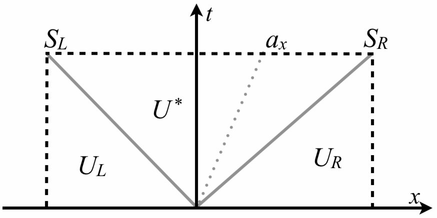
Figure 23: This figure show wave-structure of HLL Riemann solver.

B.2 HLLD Riemann solver

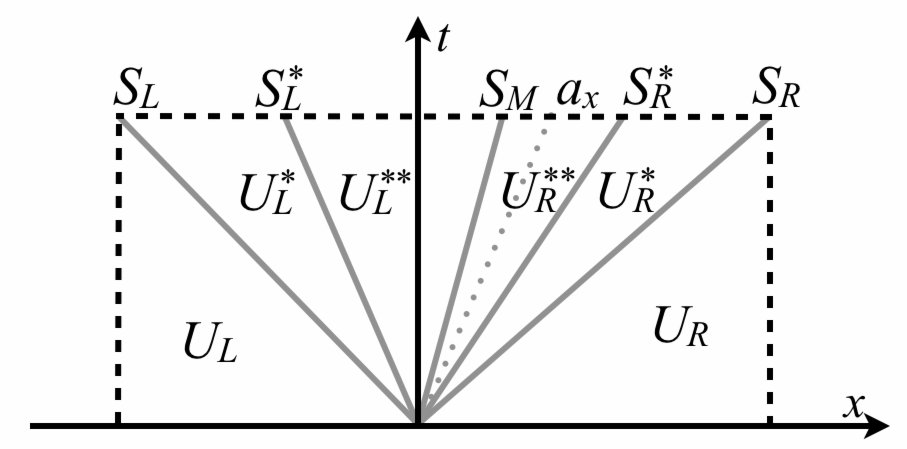
Figure 24: This figure show wave-structure of HLLD Riemann solver.

From the wave-structure of HLLD solver (Fig.24), it is clear that contact, Alfvén and fast magnetosonic waves are resolved. The fluxes at the interface for this solver are given with the following formulae

$${\cal G}^{HLLD}=\left\{\begin{array}[]{ll}{\cal F}_{L}-a_{x}{\cal U}_{L},&a_{x}<S_{L},\\ {\cal F}_{L}+(S_{L}-a_{x}){\cal U}^{\star}_{L}-S_{L}{\cal U}_{L},&S_{L}\leq a_{x}\leq S^{\star}_{L},\\ {\cal F}_{L}+(S^{\star}_{L}-a_{x}){\cal U}^{\star\star}_{L}-(S^{\star}_{L}-S_{L}){\cal U}^{\star}_{L}-S_{L}{\cal U}_{L},&S^{\star}_{L}\leq a_{x}\leq S_{M},\\ {\cal F}_{R}+(S^{\star}_{R}-a_{x}){\cal U}^{\star\star}_{R}-(S^{\star}_{R}-S_{R}){\cal U}^{\star}_{R}-S_{R}{\cal U}_{R},&S_{M}\leq a_{x}\leq S^{\star}_{R},\\ {\cal F}_{R}+(S_{R}-a_{x}){\cal U}^{\star}_{R}-S_{R}{\cal U}_{R},&S^{\star}_{R}\leq a_{x}\leq S_{R},\\ {\cal F}_{R}-a_{x}{\cal U}_{R},&S_{R}<a_{x}.\end{array}\right.$$ (60)

The wave speeds are $S_{L}=\min(v_{xL},v_{xR})-c_{\rm s}$ and $S_{R}=\max(v_{xL},v_{xR})+c_{\rm s}$, where $c_{\rm s}=\max(c_{{\rm s}L},c_{{\rm s}R})$ is the maximal signal speed in left or right state. The speed of the middle wave is defined by

$$S_{M}=\frac{P_{T,R}-P_{T,L}+\rho v_{xL}(S_{L}-v_{xL})-\rho v_{xR}(S_{R}-v_{xR})}{\rho_{L}(S_{L}-v_{xL})-\rho_{R}(S_{R}-v_{xR})},$$ (61)

$v^{\star\star}_{xK}=v^{\star}_{xK}=S_{M}$ for $K=L$, $R$, and $S^{\star}_{L}=S_{M}-|B_{x}|/\sqrt{\rho^{\star}_{L}}$ and $S^{\star}_{R}=S_{M}-|B_{x}|/\sqrt{\rho^{\star}_{R}}$. The density of both $\star$- and $\star\star$-states are

$$\rho^{\star\star}_{K}=\rho^{\star}_{K}=\rho_{K}\frac{S_{K}-v_{xK}}{S_{K}-S_{M}},$$ (62)

for $K=L,R$. The next four $\star$-states are

$$v^{\star}_{[yz]K}=v_{[yz]}-B_{x}B_{[yz]K}\frac{S_{M}-v_{xK}}{\rho_{K}(S_{K}-v_{xK})(S_{K}-S_{M})-B_{x}^{2}},$$ (63)

$$B^{\star}_{[yz]K}=B_{[yz]K}\frac{\rho_{K}(S_{K}-v_{xk})^{2}}{\rho_{K}(S_{K}-v_{xK})(S_{K}-S_{M})-B_{x}^{2}},$$ (64)

where in $[yz]$ means either $y$- or $z$-component of the corresponding 3D field. Following Miyoshi & Kusano (2005), if the last terms on the RHS result in $0/0$ uncertainty, $v^{\star}_{[yzK]}=v_{[yz]K}$ and $B^{\star}_{[yz]K}=0$, since in this case there is no shock across $S_{K}$. Finally, the remaining two $\star$-states are

$$e^{\star}_{K}=\frac{(S_{K}-v_{xK})e_{K}-P_{T_{K}}v_{xK}+P^{\star}_{T_{K}}S_{M}+B_{x}({\bf v}_{K}\cdot{\bf B}_{K}-{\bf v}^{\star}_{K}\cdot{\bf B}^{\star}_{K})}{S_{K}-S_{M}}.$$ (65)

$$P^{\star}_{T}=\frac{(S_{R}-v_{xR})\rho_{R}p_{T_{L}}-(S_{L}-v_{xL})\rho_{L}P_{T_{R}}+\rho_{L}\rho_{R}(S_{R}-v_{xR})(S_{L}-v_{xL})(v_{xR}-v_{xL})}{(S_{R}-u_{R})\rho_{R}-(S_{L}-u_{L})\rho_{L}},$$ (66)

and $P^{\star\star}_{T_{K}}=P^{\star}_{T_{K}}=P^{\star}_{T}$, for $K=L$ , $R$. The $\star\star$-states are

$$v^{\star\star}_{[yz]}=\frac{\sqrt{\rho^{\star}_{L}}v^{\star}_{[yz]L}+\sqrt{\rho^{\star}_{R}}v^{\star}_{[yz]R}+(B^{\star}_{[yz]R}-B^{\star}_{[yz]L}){\rm sign}(B_{x})}{\sqrt{\rho^{\star}_{L}}+\sqrt{\rho^{\star}_{R}}},$$ (67)

$$B^{\star\star}_{[yz]}=\frac{\sqrt{\rho^{\star}_{L}}B_{[yz]R}+\sqrt{\rho^{\star}_{R}}B_{[yz]L}+\sqrt{\rho^{\star}_{L}\rho^{\star}_{R}}(v_{[yz]R}-v_{[yz]L}){\rm sign}(B_{x})}{\sqrt{\rho^{\star}_{L}}+\sqrt{\rho^{\star}_{R}}}.$$ (68)

$$e^{\star\star}_{K}=e^{\star}_{K}\mp\sqrt{\rho^{\star}_{L}}({\bf v}^{\star}_{K}\cdot{\bf B}^{\star}_{K}-{\bf v}^{\star\star}\cdot{\bf B}^{\star\star}){\rm sign}(B_{x}).$$ (69)

In the last equations, the $-$ and $+$ on the right hand side correspond to $K=L$ and $R$ respectively. Finally, $v^{\star\star}_{[yz]K}=v^{\star\star}_{[yz]}$ and $B^{\star\star}_{[yz]K}=B^{\star\star}_{[yz]}$.

This completes the description of HLLD Riemann solver. It is clear, this solver is computationally more expensive than HLL solver due to its ability to also resolve contact and Alfvén waves, which is important in many MHD problems. In practice, it is proven to be a robust solver for many problems, and tests demonstrate it is at least as accurate as linearised-Roe solver. Furthermore, HLLD solver is possible to use with equation of state other than of ideal gas, since the equation of state in solver is used implicitly by specifying both the gas pressure and total energy.

References

- Agertz et al. (2007) Agertz O., Moore B., Stadel J., Potter D., Miniati F., Read J., Mayer L., Gawryszczak A., Kravtsov A., Nordlund Å., Pearce F., Quilis V., Rudd D., Springel V., Stone J., Tasker E., Teyssier R., Wadsley J., Walder R., 2007, MNRAS, 380, 963
- Alexander et al. (2008) Alexander R. D., Armitage P. J., Cuadra J., Begelman M. C., 2008, ApJ, 674, 927
- Balbus & Hawley (1991) Balbus S. A., Hawley J. F., 1991, ApJ, 376, 214
- Balbus & Hawley (1998) Balbus S. A., Hawley J. F., 1998, Reviews of Modern Physics, 70, 1
- Balsara (2004) Balsara D. S., 2004, ApJS, 151, 149
- Balsara & Spicer (1999) Balsara D. S., Spicer D. S., 1999, Journal of Computational Physics, 149, 270
- Børve et al. (2001) Børve S., Omang M., Trulsen J., 2001, ApJ, 561, 82
- Børve et al. (2006) Børve S., Omang M., Trulsen J., 2006, ApJ, 652, 1306
- Brandenburg (2010) Brandenburg A., 2010, MNRAS, 401, 347
- Brio & Wu (1988) Brio M., Wu C. C., 1988, Journal of Computational Physics, 75, 400
- Cha et al. (2010) Cha S., Inutsuka S., Nayakshin S., 2010, MNRAS, 403, 1165
- Cha & Whitworth (2003) Cha S., Whitworth A. P., 2003, MNRAS, 340, 73
- Colella (1990) Colella P., 1990, Journal of Computational Physics, 87, 171
- Dedner et al. (2002) Dedner A., Kemm F., Kröner D., Munz C., Schnitzer T., Wesenberg M., 2002, Journal of Computational Physics, 175, 645
- Dolag & Stasyszyn (2009) Dolag K., Stasyszyn F., 2009, MNRAS, 398, 1678
- Evans & Hawley (1988) Evans C. R., Hawley J. F., 1988, ApJ, 332, 659
- Fryxell et al. (2000) Fryxell B., Olson K., Ricker P., Timmes F. X., Zingale M., Lamb D. Q., MacNeice P., Rosner R., Truran J. W., Tufo H., 2000, ApJS, 131, 273
- Gottlieb & Shu (1998) Gottlieb S., Shu C.-W., 1998, Math. Comp, 67, 73
- Guan & Gammie (2008) Guan X., Gammie C. F., 2008, ApJS, 174, 145
- Harten et al. (1983) Harten A., Lax P. D., van Leer B., 1983, SIAM Review, 25, 35
- Inutsuka (2002) Inutsuka S., 2002, Journal of Computational Physics, 179, 238
- Lanson & Vila (2008a) Lanson N., Vila J.-P., 2008a, SIAM J. Numer. Anal., 46, 1912
- Lanson & Vila (2008b) Lanson N., Vila J.-P., 2008b, SIAM J. Numer. Anal., 46, 1935
- Lodato & Rice (2004) Lodato G., Rice W. K. M., 2004, MNRAS, 351, 630
- Maron (2005) Maron J., 2005, in Protostars and Planets V Gradient Particle Magnetohydrodynamics (GPM), a Lagrangian Particle Algorithm with Fourth-Order Gradients and Magnetic Fields. pp 8461–+
- Maron & Howes (2003) Maron J. L., Howes G. G., 2003, ApJ, 595, 564
- Mignone & Tzeferacos (2010) Mignone A., Tzeferacos P., 2010, Journal of Computational Physics, 229, 2117
- Miyoshi & Kusano (2005) Miyoshi T., Kusano K., 2005, Journal of Computational Physics, 208, 315
- Monaghan (2000) Monaghan J. J., 2000, Journal of Computational Physics, 159, 290
- Monaghan (2002) Monaghan J. J., 2002, MNRAS, 335, 843
- Monaghan (2005) Monaghan J. J., 2005, Reports on Progress in Physics, 68, 1703
- Orszag & Tang (1979) Orszag S. A., Tang C., 1979, Journal of Fluid Mechanics, 90, 129
- Plewa & Müller (1999) Plewa T., Müller E., 1999, A&A, 342, 179
- Powell et al. (1999) Powell K. G., Roe P. L., Linde T. J., Gombosi T. I., de Zeeuw D. L., 1999, Journal of Computational Physics, 154, 284
- Press et al. (1992) Press W. H., Teukolsky S. A., Vetterling W. T., Flannery B. P., 1992, Numerical recipes in C. The art of scientific computing
- Price (2007) Price D. J., 2007, Publications of the Astronomical Society of Australia, 24, 159
- Price (2010) Price D. J., 2010, MNRAS, 401, 1475
- Price & Bate (2008) Price D. J., Bate M. R., 2008, MNRAS, 385, 1820
- Price & Monaghan (2004) Price D. J., Monaghan J. J., 2004, MNRAS, 348, 123
- Price & Monaghan (2005) Price D. J., Monaghan J. J., 2005, MNRAS, 364, 384
- Price & Rosswog (2006) Price D. J., Rosswog S., 2006, Science, 312, 719
- Rosswog & Price (2007) Rosswog S., Price D., 2007, MNRAS, 379, 915
- Springel & Hernquist (2002) Springel V., Hernquist L., 2002, MNRAS, 333, 649
- Stone et al. (2008) Stone J. M., Gardiner T. A., Teuben P., Hawley J. F., Simon J. B., 2008, ApJS, 178, 137
- Swegle et al. (1995) Swegle J. W., Hicks D. L., Attaway S. W., 1995, Journal of Computational Physics, 116, 123
- Toro (1999) Toro E. F., 1999, Riemann Solvers and Numerical Methods for Fluid Dynamics : A Pratical Introduction. Springer, 2nd edition
- Tóth (2000) Tóth G., 2000, Journal of Computational Physics, 161, 605
- van Leer (2006) van Leer B., 2006, Communications in Computational Physics, 1, 192
- Vila (1999) Vila J. P., 1999, Mathematical models and Methods in Applied Sciences, 9, 161