Radiative decay of $\Lambda_{c}(2940)^{+}$ in a hadronic molecule picture

Abstract

The $\Lambda_{c}(2940)^{+}$ baryon with quantum numbers $J^{P}=\frac{1}{2}^{+}$ is considered as a molecular state composed of a nucleon and $D^{\ast}$ meson. We give predictions for the width of the radiative decay process $\Lambda_{c}(2940)^{+}\to\Lambda_{c}(2286)^{+}+\gamma$ in this interpretation. Based on our results we argue that an experimental determination of the radiative decay width of $\Lambda_{c}(2940)^{+}$ is important for the understanding of its intrinsic properties.

I Introduction

The new meson states of the $X$, $Y$ and $Z$ families, which are strongly coupled to $c\bar{c}$ quark pairs, were dominantly detected in B meson decays. At the same time, in the analysis of $\Upsilon(4S)$ decay channels two new charmed baryons ($C=+1$) denoted $\Lambda_{c}(2940)^{+}$ and $\Sigma_{c}(2800)$ were discovered. The first one of these resonances was observed by the BABAR Collaboration Aubert:2006sp and later confirmed by Belle Abe:2006rz as a resonant structure in the final state $\Sigma_{c}(2455)^{0,++}\pi^{\pm}\to\Lambda_{c}^{+}\pi^{+}\pi^{-}$ based on a 553 fb^-1 data sample collected at or near the $\Upsilon(4S)$ resonance at the KEKB collider. Both collaborations deduce values for mass and width with $m_{\Lambda_{c}}=2939.8\pm 1.3\pm 1.0$ MeV, $\Gamma_{\Lambda_{c}}=17.5\pm 5.2\pm 5.9$ MeV (BABAR Aubert:2006sp ) and $m_{\Lambda_{c}}=2938.0\pm 1.3^{+2.0}_{-4.0}$ MeV, $\Gamma_{\Lambda_{c}}=13^{+8\ +27}_{-5\ -7}$ MeV (Belle Abe:2006rz ) which are consistent with each other.

Concerning the $\Lambda_{c}(2940)^{+}$ some theoretical interpretations for this new charmed baryon resonance were already discussed in the literature. For example, in Ref. He:2006is the $\Lambda_{c}(2940)^{+}$ was regarded as a $D^{\ast 0}p$ molecular state with its spin–parity being $J^{P}=\frac{1}{2}^{-}$ or $\frac{3}{2}^{-}$. This is due to the fact that the $\Lambda_{c}(2940)^{+}$ mass is just a few MeV below the $D^{\ast 0}p$ threshold value. It was shown that the boson-exchange mechanism, involving the $\pi$, $\omega$ and $\rho$ mesons, can provide binding in such $D^{\ast 0}p$ configurations. But in a first variant of a unitary meson-baryon coupled channel model GarciaRecio:2008dp the $\Lambda_{c}(2940)^{+}$ cannot be identified with a dynamically generated resonance. In a relativized quark model Capstick:1986bm a charmed baryon state with $J^{P}=\frac{3}{2}^{+}$ or $\frac{5}{2}^{-}$ is predicted in the 2940 MeV mass region. Based on a calculation of the strong decay modes in the ${}^{3}P_{0}$ model Chen:2007xf the possibility for $\Lambda_{c}(2940)^{+}$ being the first radial excitation of the $\Lambda_{c}(2286)^{+}$ is excluded since the decay $\Lambda_{c}(2940)^{+}\to D^{0}p$ vanishes for this configuration. However, the possibility of being a $D$–wave charmed baryon with $J^{P}=\frac{1}{2}^{+}$ or $\frac{3}{2}^{+}$ was shown to be favored. Related studies concerning a conventional three-quark interpretation of the $\Lambda_{c}(2940)^{+}$ baryon can also be found in Refs. Ebert:2007nw ; Zhong:2007gp ; Cheng:2006dk ; Gerasyuta:2007un ; Roberts:2007ni ; Valcarce:2008dr ; Wang:2008vj ; Chen:2009tm .

We also recently considered the $\Lambda_{c}(2940)^{+}$ as a possible molecular state composed of a nucleon and a $D^{\ast}$ meson as based on the so-called compositeness condition Dong:2009tg . Its strong partial decay widths for the decay channel $pD^{0}$ as well as $\Sigma_{c}^{++}\pi^{-}$ and $\Sigma_{c}^{0}\pi^{+}$ were estimated applying the two different spin-parity assignments $J^{P}=\frac{1}{2}^{+}$ and $\frac{1}{2}^{-}$. For $J^{P}=\frac{1}{2}^{+}$ the sum of partial widths is consistent with present observation, while for $\frac{1}{2}^{-}$ a severe overestimate for the total decay width is obtained. Hence the choice of spin-parity $J^{P}=\frac{1}{2}^{+}$ is preferred in the molecular interpretation.

The technique for describing and treating composite hadron systems has been developed in Refs. Faessler:2007gv ; Dong:2008gb ; Dong:2009tg , where the recently observed unusual hadron states (like $D_{s0}^{\ast}(2317)$, $D_{s1}(2460)$, $X(3872)$, $Y(3940)$, $Y(4140)$, $Z(4430)$, $\Lambda_{c}(2940)^{+}$, $\Sigma_{c}(2800)$) are analyzed as hadronic molecules. The composite structure of these possible molecular states is set up by the compositeness condition $Z=0$ Weinberg:1962hj ; Efimov:1993ei ; Anikin:1995cf ; Dong:2008mt (see also Refs. Faessler:2007gv ; Dong:2008gb ; Dong:2009tg ). This condition implies that the renormalization constant of the hadron wave function is set equal to zero or that the hadron exists as a bound state of its constituents. The compositeness condition was originally applied to the study of the deuteron as a bound state of proton and neutron Weinberg:1962hj ; Dong:2008mt . Then it was extensively used in low–energy hadron phenomenology as the master equation for the treatment of mesons and baryons as bound states of light and heavy constituent quarks (see e.g. Refs. Efimov:1993ei ; Anikin:1995cf ). By constructing a phenomenological Lagrangian including the couplings of the bound state to its constituents and the constituents to other final state particles we evaluated meson–loop diagrams which describe the different decay modes of the molecular states (see details in Faessler:2007gv ; Dong:2008gb ).

Here we continue our study of the $\Lambda_{c}(2940)^{+}$ properties considering its radiative decay $\Lambda_{c}(2940)^{+}\to\Lambda_{c}(2286)^{+}+\gamma$ in the hadronic molecule approach developed in our recent paper Dong:2009tg . In particular, electromagnetic transitions are often useful for probing the internal structure of hadrons Faessler:2007gv ; Dong:2008gb ; Anikin:1995cf ; sk . Based on this previous study we choose the prefered $J^{P}=\frac{1}{2}^{+}$ assignment. As for the radiative decays of single charmed baryons in general in future one can also expect a measurement on the possible radiative decay of the $\Lambda_{c}(2940)^{+}$ baryon. Upcoming experimental facilities like a Super B factory at KEK or LHCb might provide first data in this direction. Presently data are available on radiative decays of similar hadronic compounds in the meson sector like $D_{s0}(2317)$ and $D_{s1}(2460)$ which are supposed to be molecular states composed of a heavy and a light meson — $DK$ and $D^{\ast}K$ bound state.

In the present paper we proceed as follows. In Sec. II we briefly discuss the basic notions of our approach. We discuss the effective Lagrangian for the treatment of the $\Lambda_{c}(2940)^{+}$ baryon as a superposition of the $pD^{\ast 0}$ and $nD^{\ast+}$ molecular components. Moreover, we consider the radiative decay $\Lambda_{c}(2940)^{+}\to\Lambda_{c}(2286)^{+}+\gamma$ in this section. In Sec. III we present our numerical results and, finally, in Sec. IV a short summary.

II Approach

In this section we briefly discuss the formalism for the study of the $\Lambda_{c}(2940)^{+}$ baryon. Here we adopt spin and parity quantum numbers for the $\Lambda_{c}(2940)^{+}$ with $J^{P}=\frac{1}{2}^{+}$, where consistency with the observed strong decay width of the $\Lambda_{c}(2940)^{+}$ was achieved in a hadronic molecule interpretation Dong:2009tg . Following Ref. He:2006is we consider this state as a superposition of the molecular $pD^{\ast 0}$ and $nD^{\ast+}$ components with the adjustable mixing angle $\theta$:

$$|\Lambda_{c}(2940)^{+}\rangle=\cos\theta\ |pD^{\ast 0}\rangle\ +\ \sin\theta\ |nD^{\ast+}\rangle\,.$$ (1)

The values $\sin\theta=1/\sqrt{2}$, $\sin\theta=0$ or $\sin\theta=1$ correspond to the cases of ideal mixing, of a vanishing $nD^{\ast+}$ or $pD^{\ast 0}$ component, respectively. Since the observed mass value of the $\Lambda_{c}(2940)^{+}$ with $m_{D^{\ast 0}}+m_{p}-m_{\Lambda_{c}(2940)^{+}}=5.94$ MeV and $m_{D^{\ast+}}+m_{n}-m_{\Lambda_{c}(2940)^{+}}=10.54$ MeV lies closer to the $pD^{\ast 0}$ than to the $nD^{\ast+}$ threshold, we might expect that the $|pD^{\ast 0}\rangle$ configuration is the leading component. Therefore, the mixing angle $\theta$ should be relatively small and we will vary its value from 0⁰ to 25⁰.

Our approach is based on an effective interaction Lagrangian describing the coupling of the $\Lambda_{c}(2940)^{+}$ to its constituents. We propose a setup for the $\Lambda_{c}(2940)^{+}$ in analogy to mesons consisting of a heavy quark and light antiquark, i.e. the heavy $D^{\ast}$ meson defines the center of mass of the $\Lambda_{c}(2940)^{+}$ while the light nucleon surrounds the $D^{\ast}$. The distribution of the nucleon relative to the $D^{\ast}$ meson is described by the correlation function $\Phi(y^{2})$ depending on the Jacobi coordinate $y$. The simplest form of such a Lagrangian reads

$${\cal L}_{\Lambda_{c}}(x) = \bar{\Lambda}_{c}^{+}(x)\,\gamma^{\mu}\int d^{4}y\,\Phi(y^{2})\,\Big{(}g_{\Lambda_{c}}^{0}\,\cos\theta\,D^{\ast 0}_{\mu}(x)\,p(x+y)+g_{\Lambda_{c}}^{+}\,\sin\theta\,D^{\ast+}_{\mu}(x)\,n(x+y)\Big{)}\ +\ {\rm H.c.}\,,$$ (2)

where $g_{\Lambda_{c}}^{+}$ and $g_{\Lambda_{c}}^{0}$ are the coupling constants of $\Lambda_{c}(2940)^{+}$ to the molecular $nD^{\ast+}$ and $pD^{\ast 0}$ components. Here we explicitly include isospin breaking effects by taking into account the neutron-proton and the $D^{+}-D^{0}$ mass differences. Note that in our previous analysis Dong:2009tg of the strong $\Lambda_{c}(2940)^{+}$ decays we restricted to the isospin symmetric limit. A basic requirement for the choice of an explicit form of the correlation function $\Phi(y^{2})$ is that its Fourier transform vanishes sufficiently fast in the ultraviolet region of Euclidean space to render the Feynman diagrams ultraviolet finite. We adopt a Gaussian form for the correlation function. The Fourier transform of this vertex is given by

$$\tilde{\Phi}(p_{E}^{2}/\Lambda^{2})\doteq\exp(-p_{E}^{2}/\Lambda^{2})\,,$$ (3)

where $p_{E}$ is the Euclidean Jacobi momentum. Here, $\Lambda$ is a size parameter characterizing the distribution of the nucleon in the $\Lambda_{c}(2940)^{+}$ baryon, which is a free model parameter regularizing the ultraviolet divergences of the Feynman diagrams. From the analysis of the strong decays of the $\Lambda_{c}(2940)^{+}$ baryon we found that $\Lambda\sim 1$ GeV Dong:2009tg . We might also expect that the $\Lambda_{c}(2940)^{+}$ is a quite compact molecular state which, for example, is bound by exchange of a relatively massive hadron e.g. the scalar $f_{0}(600)$. Note that similar scale parameters were also obtained in the analysis of strong and radiative decay data of possible heavy-light hadronic molecules $D_{s0}(2317)=(DK)$ and $D_{s1}(2460)=(D^{\ast}K)$ Faessler:2007gv . In the present analysis of the radiative decay of the $\Lambda_{c}(2940)^{+}$ we vary the size parameter $\Lambda$ in a wide range around this central value.

In the kinematics we first restrict to the heavy quark limit (HQL) $m_{D^{\ast}}\to\infty$ supposing that the $D^{\ast}$ meson is located in the c.m. of the $\Lambda_{c}(2940)^{+}$. It is known that in the charm sector the HQL is not always a good approximation due to possible, sizable power corrections (in our case $m_{N}/m_{D^{\ast}}$). In the numerical analysis we will estimate how large these corrections are.

The coupling constants $g_{\Lambda_{c}}^{+}$ and $g_{\Lambda_{c}}^{0}$ are the are determined by the compositeness condition Weinberg:1962hj ; Efimov:1993ei ; Anikin:1995cf ; Dong:2009tg ; Faessler:2007gv . It implies that the renormalization constant of the hadron wave function is set equal to zero with:

$$Z_{\Lambda_{c}}=1-\Sigma_{\Lambda_{c}}^{\prime}(m_{\Lambda_{c}})=0\,.$$ (4)

Here, $\Sigma_{\Lambda_{c}}^{\prime}(m_{\Lambda_{c}})$ is the derivative of the $\Lambda_{c}(2940)^{+}$ mass operator shown in Fig.1 and given by the expression:

$$\Sigma_{\Lambda_{c}}(p)=(g_{\Lambda_{c}}^{0})^{2}\cos^{2}\theta\ \Pi_{pD^{\ast 0}}(p)+(g_{\Lambda_{c}}^{+})^{2}\sin^{2}\theta\ \Pi_{nD^{\ast+}}(p)$$ (5)

where $\Pi_{pD^{\ast 0}}(p)$ and $\Pi_{nD^{\ast+}}(p)$ are the loop integrals corresponding to the $pD^{\ast 0}$ and $nD^{\ast+}$ components, respectively. Therefore, the coupling constant $g_{\Lambda_{c}}^{0}$ is fixed from Eq. (4) at the limit $\theta=0^{0}$, while the $g_{\Lambda_{c}}^{+}$ is fixed from the same equation at the limit $\theta=90^{0}$. Feynman diagrams contributing to the radiative decay of the $\Lambda_{c}(2940)^{+}$ in the hadronic molecule approach are shown in Fig.2. The $\Lambda_{c}(2940)^{+}\gamma$ final state is fed by hadron loops containing the $\Lambda_{c}(2940)^{+}$ constituents. Fig.2(a) stands for the direct coupling of the photon to the nucleon. The diagrams of Figs.2(b) and 2(c) are generated by the coupling of the photon to $D^{\ast}D$ and $D^{\ast}D^{\ast}$ meson pairs, respectively. The graph of Fig.2(d) is generated by gauging the nonlocal strong interaction Lagrangian of Eq. (2). Finally, the pole diagrams in Figs.2(e) and 2(f) originate in the direct coupling of the photon to $\Lambda_{c}(2940)^{+}$ and $\Lambda_{c}(2286)^{+}$. Note, for a real photon the pole diagrams vanish due to gauge invariance.

The phenomenological Lagrangian responsible for the full set of diagrams in Fig.2 contains the coupling of $\Lambda_{c}(2940)^{+}$ to its constituents (as already expressed in Eq. (2)) and the strong or electromagnetic interaction Lagrangians involving these constituents coupled to other fields in the loop or in the final state. These relevant interaction vertices will be defined and discussed in the following. The electromagnetic part of the Lagrangian includes the following terms:

1) $NN\gamma$ interaction which includes both minimal and nonminimal couplings

$${\cal L}_{NN\gamma}(x)=e\bar{N}(x)\,\Big{[}\,A_{\mu}(x)\,\gamma^{\mu}Q_{N}+F_{\mu\nu}(x)\,\sigma^{\mu\nu}\,\frac{k_{N}}{4M_{N}}\,\Big{]}\,N(x)\,,$$ (6)

2) $\Lambda_{c}\Lambda_{c}\gamma$ and $\Lambda_{c}^{\prime}\Lambda_{c}^{\prime}\gamma$ interaction Lagrangian (here and in the following by $\Lambda_{c}$ and $\Lambda_{c}^{\prime}$ denote the parent and daughter charmed baryons $\Lambda_{c}(2940)^{+}$ and $\Lambda_{c}(2286)^{+}$):

$${\cal L}_{\Lambda\Lambda\gamma}(x)=e\sum\limits_{\Lambda=\Lambda_{c},\Lambda_{c}^{\prime}}\,\bar{\Lambda}(x)\,A_{\mu}(x)\,\gamma^{\mu}\,\Lambda(x)\,,$$ (7)

3) $D^{\ast}D^{\ast}\gamma$ interaction is derived via minimal substitution in the free Lagrangian for charged $D^{\ast\pm}$ mesons

$${\cal L}_{D^{\ast}D^{\ast}\gamma}(x)=ieA_{\mu}(x)\Big{(}g^{\mu\beta}D^{\ast-}_{\alpha}(x)\partial^{\alpha}D^{\ast+}_{\beta}(x)-g^{\alpha\beta}D^{\ast-}_{\alpha}(x)\partial^{\mu}D^{\ast+}_{\beta}(x)\Big{)}+{\rm H.c.}\,,$$ (8)

4) $D^{\ast}D\gamma$ interaction, which contains the nonminimal coupling $g_{D^{\ast}D\gamma}$ defining the decay rate $\Gamma(D^{\ast}\to D\gamma)$ (see e.g. discussion in Ref. Dong:2008gb )

$${\cal L}_{D^{\ast}D\gamma}(x)=\frac{e}{4}g_{D^{\ast}D\gamma}\epsilon^{\mu\nu\alpha\beta}F_{\mu\nu}(x)\bar{D}^{\ast}_{\alpha\beta}(x)D(x)+{\rm H.c.}\,,$$ (9)

5) $\Lambda_{c}pD^{\ast}\gamma$ interaction Lagrangian

$${\cal L}_{\Lambda_{c}pD^{\ast}\gamma}(x) = ie\,g_{\Lambda_{c}}^{0}\,\cos\theta\,\bar{\Lambda}_{c}^{+}(x)\,\gamma^{\mu}\,D^{\ast 0}_{\mu}(x)\,\int d^{4}y\,\Phi(y^{2})\,\int\limits^{x}_{x+y}dz_{\nu}\,A^{\nu}(z)\,p(x+y)\ +\ {\rm H.c.}\,,$$ (10)

which is generated when gauging the nonlocal Lagrangian ${\cal L}_{\Lambda_{c}}$. In particular, to restore electromagnetic gauge invariance in ${\cal L}_{\Lambda_{c}}$, the proton field should be multiplied by the gauge field exponential (see further details in Refs. Anikin:1995cf ; Dong:2008mt ):

$$p(x+y)\to e^{ieI(x,x+y,P)}p(x+y)\,,~{}~{}~{}~{}~{}I(x,x+y,P)=\int\limits^{x}_{x+y}dz_{\nu}A^{\nu}(z).$$ (11)

For the derivative of $I(x,x+y,P)$ we use the path-independent prescription suggested in Ref. Mandelstam:1962mi which in turn states that the derivative of $I(x,x+y,P)$ does not depend on the path P originally used in the definition. The non-minimal substitution is therefore completely equivalent to the minimal prescription. Expanding the exponential term of $e^{ieI(x,x+y,P)}$ in powers of the electromagnetic field and keeping the linear one, we derive the Lagrangian (10) and therefore generate the vertex contained in the diagram of Fig.2(d).

In the preceding expressions we introduced several notations. $Q_{N}$ and $k_{N}$ are the nucleon charge and anomalous magnetic moments: $Q_{p}=1$, $Q_{n}=0$, $k_{p}=1.793$, $k_{n}=-1.913$. $A_{\mu}$ is the photon field. $F_{\mu\nu}=\partial_{\mu}A_{\nu}-\partial_{\nu}A_{\mu}$ and $D^{\ast}_{\alpha\beta}=\partial_{\alpha}D^{\ast}_{\beta}-\partial_{\beta}D^{\ast}_{\alpha}$ are the stress tensors of the electromagnetic field and $D^{\ast}$, respectively. The coupling constant $g_{D^{\ast}D\gamma}$ is fixed by data (central values) on the radiative decay widths $\Gamma(D^{\ast}\to D\gamma)$ PDG:2008 :

$$g_{D^{\ast\pm}D^{\pm}\gamma}=0.5\ {\rm GeV}^{-1}\,,\hskip 14.22636ptg_{D^{\ast 0}D^{0}\gamma}=2.0\ {\rm GeV}^{-1}\,.\hskip 14.22636pt$$ (12)

The relevant strong interaction Lagrangian contains two types of couplings — $ND^{\ast}\Lambda_{c}^{\prime}$ and $ND\Lambda_{c}^{\prime}$:

$${\cal L}_{ND^{\ast}\Lambda_{c}^{\prime}}=g_{ND^{\ast}\Lambda_{c}^{\prime}}\bar{N}\gamma^{\mu}\Lambda^{\prime}_{c}\bar{D}^{\ast}_{\mu}\ +\ {\rm H.c.}$$ (13)

and

$${\cal L}_{ND\Lambda_{c}^{\prime}}=g_{ND\Lambda^{\prime}_{c}}\bar{N}i\gamma_{5}\Lambda^{\prime}_{c}\bar{D}\ +\ {\rm H.c.}$$ (14)

The couplings $g_{ND^{\ast}\Lambda^{\prime}_{c}}$ and $g_{ND\Lambda^{\prime}_{c}}$ can be deduced from the phenomenological flavor-SU(4) Lagrangian Dong:2009tg ; Okubo:1975sc with

$$g_{ND\Lambda^{\prime}_{c}}=-\frac{3\sqrt{3}}{5}g_{\pi NN}\;,\;g_{ND^{\ast}\Lambda^{\prime}_{c}}=-\frac{\sqrt{3}}{2}g_{\rho NN}\;,$$ (15)

expressed in terms of the $\pi NN$ and $\rho NN$ couplings with values

$$g_{\rho NN}=6\;,\;g_{\pi NN}=13.2\;.$$ (16)

For the calculation of the electromagnetic transition amplitude between the two spin-$\frac{1}{2}$ particles $\Lambda_{c}$ and $\Lambda_{c}^{\prime}$ we have to consider the constraints of gauge invariance. In case of a general off-shell one-photon transition the invariant matrix element reads as

$${\cal M}^{\mu}(p,p^{\prime})=\bar{u}_{\Lambda_{c}^{\prime}}(p^{\prime})\Gamma^{\mu}(p,p^{\prime})u_{\Lambda_{c}}(p)\,,$$ (17)

where the vertex function $\Gamma^{\mu}(p,p^{\prime})$ is decomposed in terms of three relativistic form factors $F_{1,2,3}(q^{2})$ with the structure

$$\Gamma^{\mu}(p,p^{\prime})=F_{1}(q^{2})\gamma^{\mu}+F_{2}(q^{2})i\sigma^{\mu\nu}q_{\nu}+F_{3}(q^{2})q^{\mu}\,.$$ (18)

Here $u_{\Lambda_{c}^{\prime}}(p^{\prime})$ and $u_{\Lambda_{c}}(p)$ are the spinors of daughter and parent baryons, respectively. Due to gauge invariance with $q_{\mu}{\cal M}^{\mu}(p,p^{\prime})=0$ the form factors $F_{1}(q^{2})$ and $F_{3}(q^{2})$ are related as

$$F_{1}(q^{2})=F_{3}(q^{2})\frac{q^{2}}{m_{\Lambda_{c}}-m_{\Lambda_{c}^{\prime}}}.$$ (19)

Therefore, in the limiting case of a real photon ($q^{2}=0$) the invariant matrix element of the $\Lambda_{c}(2940)^{+}\to\Lambda_{c}(2286)^{+}+\gamma$ transition is expressed in terms of the spin-flip form factor only with

$${\cal M}^{\mu}(p,p^{\prime})=\frac{F_{\Lambda_{c}\Lambda_{c}^{\prime}\gamma}}{2m_{\Lambda_{c}}}\,\bar{u}_{\Lambda_{c}^{\prime}}(p^{\prime})\,i\,\sigma^{\mu\nu}\,q_{\nu}\,u_{\Lambda_{c}}(p)\,.$$ (20)

The coefficient $F_{\Lambda_{c}\Lambda_{c}^{\prime}\gamma}\equiv 2m_{\Lambda_{c}}F_{2}(0)$ is the effective coupling of $\Lambda_{c}(2940)^{+}\Lambda_{c}(2286)^{+}\gamma$, deduced from the set of graphs of Fig. 2, determined in our approach. This effective coupling contains the loop integrals which are evaluated using the calculational techniques developed and explicitly shown in Refs. Dong:2009tg -Dong:2008gb . Once this effective coupling is determined the final expression for the decay width is given by

$$\Gamma(\Lambda_{c}(2940)^{+}\to\Lambda_{c}(2286)^{+}+\gamma)=\frac{\alpha P^{\ast 3}}{m_{\Lambda_{c}}^{2}}\,F_{\Lambda_{c}\Lambda_{c}^{\prime}\gamma}^{2}\;,$$ (21)

where $P^{\ast}=(m_{\Lambda_{c}}^{2}-m_{\Lambda_{c}^{\prime}}^{2})/(2m_{\Lambda_{c}})$ is the three-momentum of the decay products in the rest frame of the initial $\Lambda_{c}(2940)^{+}$ baryon.

III Numerical results

For our numerical calculations the input masses of $D^{\ast 0}$, $D^{\ast+}$, $p$, $n$, $\Lambda_{c}(2940)^{+}$ and $\Lambda_{c}(2286)^{+}$ are taken from the compilation of the Particle Data Group PDG:2008 . The only free parameter in our calculation is the dimensional parameter $\Lambda$. As already stated, this parameter describes the distribution of the nucleon around the $D^{\ast}$ which is located in the center-of-mass of the $\Lambda_{c}(2940)^{+}$. Here we select $\Lambda\sim 1$ GeV, a value which is close to the scale set by the nucleon mass as usually taken in hadronic interactions sk-form . In the calculation we consider a variation of this value from 0.25 to 1.25 GeV.

In Table I we first show the dependence of the calculated couplings $g_{\Lambda_{c}}^{0}$ and $g_{\Lambda_{c}}^{+}$ on this free parameter $\Lambda$, which are fixed using the compositeness condition [see Eqs. (4) and (5)]. We find that the difference in the binding energies ($M_{p}+M_{D^{\ast 0}}-m_{\Lambda_{c}(2940)^{+}}=5.9$ MeV and $M_{n}+M_{D^{\ast+}}-m_{\Lambda_{c}(2940)^{+}}=10.5$ MeV) leads to some deviation between the respective coupling constants $g_{\Lambda_{c}}^{0}$ and $g_{\Lambda_{c}}^{+}$. Also decreasing of the scale parameter $\Lambda$ leads to decreasing of the couplings $g_{\Lambda_{c}}^{0}$ and $g_{\Lambda_{c}}^{+}$. One can see that at values of $\Lambda\leq 0.75$ GeV the couplings are quite suppressed, so the preferred region for the fixing parameters $\Lambda$ is around 1 GeV. In Tables II and III we present the numerical results for the effective coupling constant $F_{\Lambda_{c}\Lambda_{c}^{\prime}\gamma}$ and for the resulting radiative decay width of the process $\Lambda_{c}(2940)^{+}\rightarrow\Lambda_{c}(2286)^{+}+\gamma$. The predictions for the decay width are given for selected values of $\Lambda=0.25$, $0.4$, $0.5$, $0.75$, $1$, $1.25$ GeV and for a variety of mixing angles $\theta$ in the interval $(0-25)^{0}$. Our results are rather sensitive to a variation of the scale parameter $\Lambda$. This should be obvious since the ultraviolet divergence of the diagrams is regularized by the cutoff $\Lambda$. Again at relatively small values of $\Lambda$ the predictions for the decay parameters are very small. The results also possess a pronounced sensitivity on a variation of the mixing parameter $\theta$. An increase of $\theta$ leads to a suppression of the effective coupling and hence the decay width. The range of the estimated decay width is rather wide and varies from several to hundred keV. This is mainly due to the nontrivial cancellation between diagrams involving the $|pD^{\ast 0}\rangle$ and the $|nD^{\ast+}\rangle$ components in the loops. For illustration of this behavior in Table 4 we present the contributions of the different diagrams to the effective coupling at values of $\Lambda=1$ GeV and $\theta=10^{0}$. All contributions involving the $|nD^{\ast+}\rangle$ component are destructive in comparison to the leading contribution giving by the $|pD^{\ast 0}\rangle$ component in the diagram of Fig.2(a). This leads to a suppression of the effective coupling and the width when the fraction of the $|nD^{\ast+}\rangle$ component (or the value of the mixing angle $\theta$) is increased. Our final comment concerns an estimate of power corrections to the decay rate due to the shift of the position of the $D^{\ast}$ from the $\Lambda_{c}(2940)^{+}$ c.m. These corrections depend on the scale parameter $\Lambda$. We found that for $\Lambda=1$ GeV these corrections are up to 10% depending on the mixing angle $\theta$. Varying $\Lambda$ from 1 GeV to 0.25 GeV these corrections increase up to 30%, while they are reduced when $\Lambda$ increases. For completeness we present the results including power corrections for the specific values of the model parameters $\Lambda=1$ GeV and $\theta=10^{0}$. They are given in Table 4 in brackets.

IV Summary

To summarize, we pursue a hadronic molecule interpretation of the recently observed charmed baryon $\Lambda_{c}(2940)^{+}$ studying its consequences for the radiative decay mode $\Lambda_{c}(2286)^{+}\gamma$ for spin-parity $J^{P}=\frac{1}{2}^{+}$. In the present scenario the $\Lambda_{c}(2940)^{+}$ baryon is described by a superposition of $|pD^{\ast 0}\rangle$ and $|nD^{\ast+}\rangle$ components with the explicit admixture expressed by the mixing angle $\theta$. Our numerical results for the radiative decay widths show that the contribution of diagram Fig.2(a) gives the leading contribution while those of Figs. 2(b), 2(c) and 2(d) are subleading but non-negligible. The diagrams of Fig.2(e) and 2(f) vanish for real photons and, therefore, do not contribute to the process $\Gamma(\Lambda_{c}(2940)^{+}\to\Lambda_{c}(2286)^{+}+\gamma)$. The calculated radiative decay widths display a sizable sensitivity to the mixing angle $\theta$ and to the scale parameter $\Lambda$. Especially the cancellation between the contributions of the diagrams Figs.2(a)-2(d) results in a rather pronounced $\theta$-dependence. This effect can provide a stringent constraint on the role of the two molecular components $pD^{\ast 0}$ and $nD^{\ast+}$ in the $\Lambda_{c}(2940)^{+}$ resonance. Possible future measurements of the radiative decay width can provide further insights into the structure of the $\Lambda_{c}(2940)^{+}$ state. New facilities like the Super B factory at KEK or LHCb might have the capability to reach the sensitivity to detect radiative decays of charmed baryons in the keV regime.

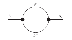
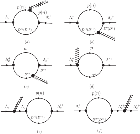
Figure 1: Diagram describing the $\Lambda_{c}(2940)^{+}$ mass operator.

Figure 2: Diagrams contributing to the radiative decay process $\Lambda_{c}(2940)^{+}\to\Lambda_{c}(2286)^{+}\gamma$.

Table I. Couplings $g_{\Lambda_{c}}^{0}$ and $g_{\Lambda_{c}}^{+}$.

$\Lambda$ (GeV)	$g_{\Lambda_{c}}^{0}$	$g_{\Lambda_{c}}^{+}$
0.25	3 $\times 10^{-5}$	4 $\times 10^{-5}$
0.4	1.2 $\times 10^{-2}$	1.6 $\times 10^{-2}$
0.5	0.09	0.10
0.75	0.56	0.67
1	1.09	1.29
1.25	1.51	1.74

Table II. Effective coupling constant $F_{\Lambda_{c}\Lambda_{c}^{\prime}\gamma}$.

$\theta$	$\Lambda$ (GeV)
(in grad)	$0.25$	$0.4$	$0.5$	$0.75$	$1$	$1.25$
0	0.26	0.46	0.61	0.83	0.93	0.97
5	0.24	0.42	0.56	0.74	0.82	0.85
10	0.22	0.37	0.50	0.66	0.71	0.72
15	0.21	0.33	0.43	0.56	0.60	0.58
20	0.16	0.28	0.37	0.46	0.47	0.44
25	0.13	0.22	0.30	0.36	0.35	0.30

Table III. Radiative decay width of $\Lambda_{c}(2940)^{+}$ in keV.

$\theta$	$\Lambda$ (GeV)
(in grad)	$0.25$	$0.4$	$0.5$	$0.75$	$1$	$1.25$
0	11.1	35.4	61.7	113.1	142.7	156.8
5	9.2	29.2	51.0	91.5	112.2	119.4
10	7.4	23.2	40.6	71.0	83.9	85.5
15	5.7	17.6	30.8	52.1	58.6	56.2
20	4.1	12.5	22.0	35.5	37.1	32.4
25	2.7	8.1	14.4	21.7	20.1	14.7

Table IV. Contributions of the diagrams Figs. 2(a)-(d) to $F_{\Lambda_{c}\Lambda_{c}^{\prime}\gamma}$ at $\Lambda=1$ GeV and $\theta=10^{0}$.

Numbers in brackets include power corrections discussed in the text.

Diagram	$F_{\Lambda_{c}\Lambda_{c}^{\prime}\gamma}$
	$pD^{\ast 0}$	$nD^{\ast+}$	$pD^{\ast 0}+nD^{\ast+}$
Fig.2(a)	1.00 (1.17)	$-$ 0.16 ($-$0.40)	0.84 (0.77)
Fig.2(b)	$-$ 0.13 ($-$ 0.25)	$-$ 0.01 ($-$ 0.01)	$-$ 0.14 ($-$ 0.26)
Fig.2(c)	0 (0)	$-$ 0.04 ($-$ 0.04)	$-$ 0.04 ($-$ 0.04)
Fig.2(d)	0.05 (0.13)	0 (0.08)	0.05 (0.21)
Total	0.92 (1.05)	$-$ 0.21 ($-$ 0.37)	0.71 (0.68)