Renormalization of masses of sterile neutrinos in the ν𝜈\nuMSM

Ananda Roy ananda.roy@epfl.ch Indian Institute of Technology Kanpur, Kanpur, Uttar Pradesh 208016,India Institut de Théorie des Phénomènes Physiques, EPFL, CH-1015 Lausanne, Switzerland
Abstract

The quasi-degeneracy of heavier sterile neutrino masses in the Neutrino Minimal Standard Model (ν𝜈\nuMSM) facilitates the production of lepton asymmetry below the electroweak scale. The first order loop corrections to this mass-difference has been computed in this work along with a numerical estimate of the contribution.

ν𝜈\nuMSM, loop corrections, mass difference, neutrino physics
pacs:
11.10.Hi,12.10.-g,12.60.-i,13.15.+g

I Introduction

A renormalizable extension of the Standard Model (SM), the ν𝜈\nuMSM extends the existing SM of particle physics by three sterile neutrinos, which are singlets under the SM gauge group. The ν𝜈\nuMSM attempts to address the various unresolved issues of the SM Asaka:2005an ; Asaka:2005pn ; Shaposhnikov:2008pf ; Bezrukov:2007ep (for a review see Boyarsky:2009ix ), one of them being dark matter production. The lepton asymmetry, produced at the same time as the generation of the dark matter sterile neutrinos (at temperature of 100similar-toabsent100\sim 100 MeV), affects their spectrum and number density (see Shi:1998km ; Asaka:2006nq ; Laine:2008pg ). Upon comparison of theoretical computation of the abundance of dark matter sterile neutrino with cosmological and astrophysical observations, the lepton asymmetry (ΔLΔ𝐿\Delta L) is required to be much larger than the baryon asymmetry (ΔΔ\DeltaB): ΔLΔB3×105Δ𝐿Δ𝐵3superscript105\frac{\Delta L}{\Delta B}\geq 3\times 10^{5}, where ΔB1010similar-toΔ𝐵superscript1010\Delta B\sim 10^{-10}. 111Different possible ways to modify this requirement may be found in Shaposhnikov:2006xi ; Kusenko:2006rh ; Anisimov:2008qs ; Bezrukov:2009yw ; Bezrukov:2008ut .

The high value of the lepton-asymmetry can be created provided the masses of the heavier sterile neutrinos in the ν𝜈\nuMSM are almost degenerate. Moreover, the mass-difference that leads to the requisite value of the lepton asymmetry must be much lower than the active neutrino mass-difference Shaposhnikov:2008pf ; ananda2 . In an accompanying paper ananda2 , we discussed the naturalness of the fine-tuning required for satisfying the leptogenesis and active neutrino oscillation observations from the perspective of the renormalization group (RG) evolution of the ν𝜈\nuMSM parameters. A complete analysis of the effect of mass-difference on leptogenesis, however, requires the computation of the physical mass-difference. This is the purpose of the present work, where we compute the radiative corrections to the mass-difference at the one loop level. For a review of the generalized on-shell renormalization procedure for Majorana neutrino theories, see Almasy:2009kn .

The paper is organized as follows: in section II, we review the Lagrangian of the ν𝜈\nuMSM, along with the definitions of the different parameters. In section III, we describe our formalism of computation of loop corrections and compute the various contributions. In section IV, we compute the mass difference with the loop corrections taken into account, while numerical estimates are given in V. Finally, in section VI, we summarize our results.

II The ν𝜈\nuMSM Lagrangian and Relevant Mass-Matrix

We use the Lagrangian of the ν𝜈\nuMSM in the parametrization Shaposhnikov:2008pf ; ananda2 ; Shaposhnikov:2006nn . In addition, considering the fact that the sterile neutrino Yukawa couplings are much smaller than the gauge couplings and neglecting the numerically much smaller charged lepton Yukawa couplings, we choose a basis for the leptonic doublets, in which the Lagrangian has the following simple form:

νMSM=0+Δ,subscript𝜈𝑀𝑆𝑀subscript0Δ{\cal L}_{\nu MSM}={\cal L}_{0}+\Delta{\cal L}, (1)
0=SM+I=2,3NI¯iμγμNI+(f2l2¯N2\displaystyle{\cal L}_{0}={\cal L}_{SM}+\sum_{I=2,3}\overline{N_{I}}i\partial_{\mu}\gamma^{\mu}N_{I}+(f_{2}\overline{l_{2}}N_{2}
+f3l3¯N3)ϕ~MN2c¯N3+h.c.,\hskip 56.9055pt+f_{3}\overline{l_{3}}N_{3})\tilde{\phi}-M\overline{N_{2}^{c}}N_{3}+h.c., (2)
Δ=f23l2¯N3Φ~ΔM2I=2,3NIc¯NI+h.c.,formulae-sequenceΔsubscript𝑓23¯subscript𝑙2subscript𝑁3~ΦΔ𝑀2subscript𝐼23¯superscriptsubscript𝑁𝐼𝑐subscript𝑁𝐼𝑐\Delta{\cal L}=f_{23}\overline{l_{2}}N_{3}\tilde{\Phi}-\frac{\Delta M}{2}\sum_{I=2,3}\overline{N_{I}^{c}}N_{I}+h.c., (3)

where NIsubscript𝑁𝐼N_{I} are the right handed singlet leptons (I=2,3𝐼23I=2,3), ϕitalic-ϕ\phi and l2,3subscript𝑙23l_{2,3} are the Higgs and the lepton doublets respectively, M𝑀M is the common mass of the two heavy neutral fermions, ΔMΔ𝑀\Delta M is the diagonal element of the Majorana mass matrix, ϕ~i=ϵijϕjsubscript~italic-ϕ𝑖subscriptitalic-ϵ𝑖𝑗subscriptsuperscriptitalic-ϕ𝑗\tilde{\phi}_{i}=\epsilon_{ij}\phi^{*}_{j}, M and ΔMΔ𝑀\Delta M are taken to be real. The Yukawa couplings f2,f3subscript𝑓2subscript𝑓3f_{2},f_{3} can be chosen to be real by suitably defining the phases of l2,l3subscript𝑙2subscript𝑙3l_{2},l_{3}, while the f23subscript𝑓23f_{23} is complex, with a phase of n𝑛n. The relation between f2,f3subscript𝑓2subscript𝑓3f_{2},f_{3} and hαIsubscript𝛼𝐼h_{\alpha I} introduced in Shaposhnikov:2008pf ; ananda2 can be found by comparing eqs. (2) and (3) with eqs. (2) and (3) of ananda2 .

We have omitted the dark matter sterile neutrino N1subscript𝑁1N_{1} from the Lagrangian as its influence on the problem we are interested in is negligibly small Shaposhnikov:2008pf .

We will use unitary gauge (Φ=12(0v+h)TΦ12superscript0𝑣𝑇\Phi=\frac{1}{\sqrt{2}}(0\ v+h)^{T}) to reduce the computational complexity. Here v𝑣v is the vacuum expectation value of the Higgs boson and is taken to be 246 GeV. For a list of conventions used for the computation, see appendix A.

Using the Euler-Lagrange’s equation of motion, we get the Dirac equation for the system of particles as follows:

i∂̸(N2RN3Rν2Lcν3LcN2RcN3Rcν2Lν3L)(0MνMν0)(N2RN3Rν2Lcν3LcN2RcN3Rcν2Lν3L)=0,𝑖not-partial-differentialmatrixsubscript𝑁2𝑅subscript𝑁3𝑅superscriptsubscript𝜈2𝐿𝑐superscriptsubscript𝜈3𝐿𝑐superscriptsubscript𝑁2𝑅𝑐superscriptsubscript𝑁3𝑅𝑐subscript𝜈2𝐿subscript𝜈3𝐿matrix0subscript𝑀𝜈superscriptsubscript𝑀𝜈0matrixsubscript𝑁2𝑅subscript𝑁3𝑅superscriptsubscript𝜈2𝐿𝑐superscriptsubscript𝜈3𝐿𝑐superscriptsubscript𝑁2𝑅𝑐superscriptsubscript𝑁3𝑅𝑐subscript𝜈2𝐿subscript𝜈3𝐿0i\not{\partial}\begin{pmatrix}N_{2R}\\ N_{3R}\\ \nu_{2L}^{c}\\ \nu_{3L}^{c}\\ N_{2R}^{c}\\ N_{3R}^{c}\\ \nu_{2L}\\ \nu_{3L}\end{pmatrix}-\begin{pmatrix}0&M_{\nu}\\ M_{\nu}^{\dagger}&0\end{pmatrix}\begin{pmatrix}N_{2R}\\ N_{3R}\\ \nu_{2L}^{c}\\ \nu_{3L}^{c}\\ N_{2R}^{c}\\ N_{3R}^{c}\\ \nu_{2L}\\ \nu_{3L}\end{pmatrix}=0, (4)

where

Mν=(ΔMMvf220MΔMvf232vf32vf22vf232000vf3200).subscript𝑀𝜈matrixΔ𝑀𝑀𝑣subscript𝑓220𝑀Δ𝑀𝑣superscriptsubscript𝑓232𝑣subscript𝑓32𝑣subscript𝑓22𝑣superscriptsubscript𝑓232000𝑣subscript𝑓3200M_{\nu}=\begin{pmatrix}\Delta M&M&\frac{-vf_{2}}{\sqrt{2}}&0\\ M&\Delta M&\frac{-vf_{23}^{*}}{\sqrt{2}}&\frac{-vf_{3}}{\sqrt{2}}\\ \frac{-vf_{2}}{\sqrt{2}}&\frac{-vf_{23}^{*}}{\sqrt{2}}&0&0\\ 0&\frac{-vf_{3}}{\sqrt{2}}&0&0\end{pmatrix}. (5)

At the tree level, the eigenvectors of MνMνsuperscriptsubscript𝑀𝜈subscript𝑀𝜈M_{\nu}^{\dagger}M_{\nu} up to first order in Yukawa couplings with eigenvalues of Mνsubscript𝑀𝜈M_{\nu} up to second order in the same are obtained by perturbative computation and are listed in the appendix B (see Justine ).

The mass-difference between the sterile neutrino flavors were shown to be Shaposhnikov:2008pf :

δmtree=|m2|M,𝛿subscript𝑚𝑡𝑟𝑒𝑒superscript𝑚2𝑀\delta m_{tree}=\frac{|m^{2}|}{M}, (6)

where

m2f2f23v2+2MΔM.superscript𝑚2subscript𝑓2subscript𝑓23superscript𝑣22𝑀Δ𝑀m^{2}\equiv f_{2}f_{23}v^{2}+2M\Delta M. (7)

The aim of the paper is to compute the first order loop corrections to this mass difference.

Also, the active neutrino mass-difference (ΔmνΔsubscript𝑚𝜈\Delta m_{\nu}) may be solved at the tree-level to be Shaposhnikov:2008pf :

Δmν=f2|f23|v2M.Δsubscript𝑚𝜈subscript𝑓2subscript𝑓23superscript𝑣2𝑀\Delta m_{\nu}=\frac{f_{2}|f_{23}|v^{2}}{M}. (8)

III Loop Corrections

III.1 Propagator

Consider the propagator for the system of active and sterile neutrinos:

SF(p)=iΣ,subscript𝑆𝐹𝑝𝑖italic-p̸ΣS_{F}(p)=\frac{i}{\not{p}-{\cal M}-\Sigma}, (9)

where ΣΣ\Sigma represents the first order loop correction to the mass matrix {\cal M}. It is useful to keep in mind that {\cal M} and ΣΣ\Sigma represent the mass-matrix and the loop corrections of the complete system of 2 active and 2 sterile neutrinos, and hence are 8×8888\times 8 matrices. As usual, mass eigenvalues are given at the one loop level by the poles of the propagator.

Including only one particle irreducible diagrams for the computation, it is easy to see that only the following loop correction matrix elements are relevant: Σss,Σas,ΣsaandΣaasubscriptΣ𝑠𝑠subscriptΣ𝑎𝑠subscriptΣ𝑠𝑎andsubscriptΣ𝑎𝑎\Sigma_{ss},\Sigma_{as},\Sigma_{sa}\ \text{and}\ \Sigma_{aa},where

Σss=(N2R|Σ|N2RN2R|Σ|N3RN3R|Σ|N2RN3R|Σ|N3R)subscriptΣ𝑠𝑠matrixquantum-operator-productsubscript𝑁2𝑅Σsubscript𝑁2𝑅quantum-operator-productsubscript𝑁2𝑅Σsubscript𝑁3𝑅quantum-operator-productsubscript𝑁3𝑅Σsubscript𝑁2𝑅quantum-operator-productsubscript𝑁3𝑅Σsubscript𝑁3𝑅\Sigma_{ss}=\begin{pmatrix}\langle N_{2R}|\Sigma|N_{2R}\rangle&\langle N_{2R}|\Sigma|N_{3R}\rangle\\ \langle N_{3R}|\Sigma|N_{2R}\rangle&\langle N_{3R}|\Sigma|N_{3R}\rangle\end{pmatrix} (10)

and so on. Here the subscripts s,a𝑠𝑎s,a represent sterile and active flavors respectively.

III.2 Loop correction to active neutrino propagators:
Computation of ΣaasubscriptΣ𝑎𝑎\Sigma_{aa}

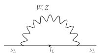
Considering diagrams that give up to quadratic contribution in Yukawa coupling, we find that the only possible contribution comes from the internal W and Z boson loops. The following figure (Fig. 1) represents the loop-correction to the active neutrino propagator.
Refer to caption
Figure 1: Contribution to active neutrino propagator from W,Z boson loop.

Performing the one-loop computation using dimensional regularization, we find that

ν2L|Σ|ν2L=(4π)2[p2v2(1+lnμ2MW2)p22v2(1+lnμ2MZ2)\displaystyle\langle\nu_{2L}|\Sigma|\nu_{2L}\rangle=\frac{\not{p}}{(4\pi)^{2}}\Big{[}-\frac{p^{2}}{v^{2}}(1+\ln\frac{\mu^{2}}{M_{W}^{2}})-\frac{p^{2}}{2v^{2}}(1+\ln\frac{\mu^{2}}{M_{Z}^{2}})
+3g2+g224].\hskip 56.9055pt+\frac{3g^{2}+g^{\prime 2}}{24}\Big{]}. (11)

Define:

C1=1(4π)2[p2v2(1+lnμ2MW2)p22v2(1+lnμ2MZ2)+3g2+g224].subscript𝐶11superscript4𝜋2delimited-[]superscript𝑝2superscript𝑣21superscript𝜇2superscriptsubscript𝑀𝑊2superscript𝑝22superscript𝑣21superscript𝜇2superscriptsubscript𝑀𝑍23superscript𝑔2superscript𝑔224C_{1}=\frac{1}{(4\pi)^{2}}\Big{[}-\frac{p^{2}}{v^{2}}(1+\ln\frac{\mu^{2}}{M_{W}^{2}})-\frac{p^{2}}{2v^{2}}(1+\ln\frac{\mu^{2}}{M_{Z}^{2}})+\frac{3g^{2}+g^{\prime 2}}{24}\Big{]}. (12)

Since the active neutrino masses are much smaller than the Higgs vacuum expectation value, we can assume that p2v2much-less-thansuperscript𝑝2superscript𝑣2p^{2}\ll v^{2}, implying

C1=1(4π)23g2+g224.subscript𝐶11superscript4𝜋23superscript𝑔2superscript𝑔224C_{1}=\frac{1}{(4\pi)^{2}}\frac{3g^{2}+g^{\prime 2}}{24}. (13)

Thus,

ν2L|Σ|ν2L=C1.quantum-operator-productsubscript𝜈2𝐿Σsubscript𝜈2𝐿italic-p̸subscript𝐶1\langle\nu_{2L}|\Sigma|\nu_{2L}\rangle=\not{p}C_{1}. (14)

Analogous computation shows:

ν3L|Σ|ν3L=C1.quantum-operator-productsubscript𝜈3𝐿Σsubscript𝜈3𝐿italic-p̸subscript𝐶1\langle\nu_{3L}|\Sigma|\nu_{3L}\rangle=\not{p}C_{1}. (15)

In absence of terms contributing to the mixing between ν2subscript𝜈2\nu_{2} and ν3subscript𝜈3\nu_{3}, the lowest order contribution to the loop correction matrix may be written as follows:

Σaa=C1(1001).subscriptΣ𝑎𝑎italic-p̸subscript𝐶1matrix1001\Sigma_{aa}=\not{p}C_{1}\begin{pmatrix}1&0\\ 0&1\end{pmatrix}. (16)

III.3 Loop Correction to the Sterile Neutrino propagators:
Computation of ΣsssubscriptΣ𝑠𝑠\Sigma_{ss}

The sterile neutrino propagator receives contributions from the internal Higgs loop in addition to W and Z boson loops. From here on, we use the intuitive notation that Σw,z,h,tsubscriptΣ𝑤𝑧𝑡\Sigma_{w,z,h,t} respectively represent the contribution to the loop-correction ΣΣ\Sigma from W, Z, Higgs-boson loop and tadpole graphs.

III.3.1 Contribution from the W boson loop
Refer to caption
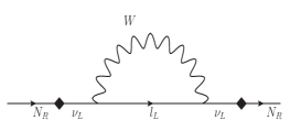
Figure 2: Contribution to sterile neutrino propagator from W boson loop; N, ν𝜈\nu represent the different possible flavors.

The contribution coming from the W boson loop is represented in Fig. 2 and is given by

N2R|Σw|N2R=f22(4π)2[12(lnμ2MW2+1)+g2v224p2].quantum-operator-productsubscript𝑁2𝑅subscriptΣ𝑤subscript𝑁2𝑅superscriptsubscript𝑓22superscript4𝜋2italic-p̸delimited-[]12superscript𝜇2superscriptsubscript𝑀𝑊21superscript𝑔2superscript𝑣224superscript𝑝2\langle N_{2R}|\Sigma_{w}|N_{2R}\rangle=\frac{f_{2}^{2}}{(4\pi)^{2}}\not{p}\Big{[}-\frac{1}{2}(\ln\frac{\mu^{2}}{M_{W}^{2}}+1)+\frac{g^{2}v^{2}}{24p^{2}}\Big{]}. (17)

III.3.2 Contribution from Z boson loop
Refer to caption
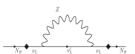
Figure 3: Contribution to sterile neutrino propagator from Z boson loop.

Fig. 3 represents the contribution from the Z-boson loop. Performing the computation, we get

N2R|Σz|N2R=f22(4π)2[14(lnμ2MZ2+1)+(g2+g2)v248p2].quantum-operator-productsubscript𝑁2𝑅subscriptΣ𝑧subscript𝑁2𝑅superscriptsubscript𝑓22superscript4𝜋2italic-p̸delimited-[]14superscript𝜇2superscriptsubscript𝑀𝑍21superscript𝑔2superscript𝑔2superscript𝑣248superscript𝑝2\langle N_{2R}|\Sigma_{z}|N_{2R}\rangle=\frac{f_{2}^{2}}{(4\pi)^{2}}\not{p}\Big{[}-\frac{1}{4}(\ln\frac{\mu^{2}}{M_{Z}^{2}}+1)+\frac{(g^{2}+g^{\prime 2})v^{2}}{48p^{2}}\Big{]}. (18)

III.3.3 Contribution from the Higgs boson loop
Refer to caption
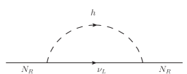
Figure 4: Contribution to sterile neutrino propagator from Higgs boson loop.

The above figure (Fig. 4) shows the contribution from the Higgs loop, which leads to

N2R|Σh|N2R=f22(4π)2[12lnμ2mH2+14].quantum-operator-productsubscript𝑁2𝑅subscriptΣsubscript𝑁2𝑅superscript𝑓2italic-p̸2superscript4𝜋2delimited-[]12superscript𝜇2superscriptsubscript𝑚𝐻214\langle N_{2R}|\Sigma_{h}|N_{2R}\rangle=\frac{-f^{2}\not{p}}{2(4\pi)^{2}}\Big{[}\frac{1}{2}\ln\frac{\mu^{2}}{m_{H}^{2}}+\frac{1}{4}\Big{]}. (19)

III.3.4 Matrix Element representing the loop contribution

The total loop-correction will be the sum of the aforementioned contributions. Thus,

Σss=(F1~+F2~)(f2f2f23f2f23f32+|f23|2),subscriptΣ𝑠𝑠italic-p̸~subscript𝐹1~subscript𝐹2matrixsuperscript𝑓2subscript𝑓2superscriptsubscript𝑓23subscript𝑓2subscript𝑓23superscriptsubscript𝑓32superscriptsubscript𝑓232\Sigma_{ss}=\not{p}(\tilde{F_{1}}+\tilde{F_{2}})\begin{pmatrix}f^{2}&f_{2}f_{23}^{*}\\ f_{2}f_{23}&f_{3}^{2}+|f_{23}|^{2}\end{pmatrix}, (20)

where

F1~=12(4π)2[12lnμ2mH2+14],~subscript𝐹112superscript4𝜋2delimited-[]12superscript𝜇2superscriptsubscript𝑚𝐻214\displaystyle\tilde{F_{1}}=\frac{-1}{2(4\pi)^{2}}\Big{[}\frac{1}{2}\ln\frac{\mu^{2}}{m_{H}^{2}}+\frac{1}{4}\Big{]}, (21)
F2~=1(4π)2[14(lnμ2MZ2+1)+(g2+g2)v248p2]~subscript𝐹21superscript4𝜋2delimited-[]14superscript𝜇2superscriptsubscript𝑀𝑍21superscript𝑔2superscript𝑔2superscript𝑣248superscript𝑝2\tilde{F_{2}}=\frac{1}{(4\pi)^{2}}\Big{[}-\frac{1}{4}(\ln\frac{\mu^{2}}{M_{Z}^{2}}+1)+\frac{(g^{2}+g^{\prime 2})v^{2}}{48p^{2}}\Big{]}
+1(4π)2[12(lnμ2MW2+1)+g2v224p2].1superscript4𝜋2delimited-[]12superscript𝜇2superscriptsubscript𝑀𝑊21superscript𝑔2superscript𝑣224superscript𝑝2\hskip 56.9055pt+\frac{1}{(4\pi)^{2}}\Big{[}-\frac{1}{2}(\ln\frac{\mu^{2}}{M_{W}^{2}}+1)+\frac{g^{2}v^{2}}{24p^{2}}\Big{]}. (22)

III.4 Loop Correction to the Active-Sterile Neutrino propagator: Computation of ΣassubscriptΣ𝑎𝑠\Sigma_{as} and ΣsasubscriptΣ𝑠𝑎\Sigma_{sa}

The active-sterile neutrino propagator receives similar contribution from the W and Z boson loops on the external active neutrino leg and in addition receives contributions from tadpoles. We consider only the top quark loop among the possible fermion loops in the tadpole graphs.

III.4.1 Contribution from W boson
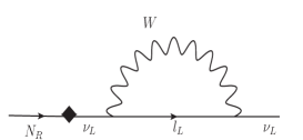
Refer to caption
Figure 5: Contribution to active-sterile neutrino propagator from W boson loop.

The W-boson loop contribution is represented by Fig. 5 and it is given by

ν2L|Σw|N2R=f2v21(4π)2[p2v2(1+lnμ2MW2)+g212].quantum-operator-productsubscript𝜈2𝐿subscriptΣ𝑤subscript𝑁2𝑅subscript𝑓2𝑣21superscript4𝜋2delimited-[]superscript𝑝2superscript𝑣21superscript𝜇2superscriptsubscript𝑀𝑊2superscript𝑔212\langle\nu_{2L}|\Sigma_{w}|N_{2R}\rangle=-\frac{f_{2}v}{\sqrt{2}}\frac{1}{(4\pi)^{2}}\Big{[}-\frac{p^{2}}{v^{2}}(1+\ln\frac{\mu^{2}}{M_{W}^{2}})+\frac{g^{2}}{12}\Big{]}. (23)

III.4.2 Contribution from Z boson loop

Refer to caption
Figure 6: Contribution to active-sterile neutrino propagator from Z boson loop.

Fig. 6 represents the contribution from the Z boson loop, which leads to

ν2L|Σz|N2R=f2v21(4π)2[p22v2(1+lnμ2MZ2)+g2+g224].quantum-operator-productsubscript𝜈2𝐿subscriptΣ𝑧subscript𝑁2𝑅subscript𝑓2𝑣21superscript4𝜋2delimited-[]superscript𝑝22superscript𝑣21superscript𝜇2superscriptsubscript𝑀𝑍2superscript𝑔2superscript𝑔224\langle\nu_{2L}|\Sigma_{z}|N_{2R}\rangle=-\frac{f_{2}v}{\sqrt{2}}\frac{1}{(4\pi)^{2}}\Big{[}-\frac{p^{2}}{2v^{2}}(1+\ln\frac{\mu^{2}}{M_{Z}^{2}})+\frac{g^{2}+g^{\prime 2}}{24}\Big{]}. (24)

III.4.3 Contribution from tadpole graphs
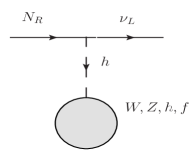
Refer to caption
Figure 7: Contribution to active-sterile neutrino propagator from tadpole graphs.

The tadpole contribution to the active-sterile neutrino propagator is represented by Fig. 7, which leads to

ν2L|Σt|N2R=f2(4π)2[3mH222vlnμ2mH26MW42vmH2lnμ2MW2\langle\nu_{2L}|\Sigma_{t}|N_{2R}\rangle=\frac{f_{2}}{(4\pi)^{2}}\Big{[}-\frac{3m_{H}^{2}}{2\sqrt{2}v}\ln\frac{\mu^{2}}{m_{H}^{2}}-\frac{6M_{W}^{4}}{\sqrt{2}vm_{H}^{2}}\ln\frac{\mu^{2}}{M_{W}^{2}}
3MZ42vmH2lnμ2MZ2+12mf42mH2vlnμ2mf2].\hskip 85.35826pt-\frac{3M_{Z}^{4}}{\sqrt{2}vm_{H}^{2}}\ln\frac{\mu^{2}}{M_{Z}^{2}}+\frac{12m_{f}^{4}}{\sqrt{2}m_{H}^{2}v}\ln\frac{\mu^{2}}{m_{f}^{2}}\Big{]}. (25)

III.4.4 Matrix Element representing the loop contribution

Thus,

Σas=(K1+K2)(f2f230f3)=(K1+K2)C,subscriptΣ𝑎𝑠subscript𝐾1subscript𝐾2matrixsubscript𝑓2superscriptsubscript𝑓230subscript𝑓3subscript𝐾1subscript𝐾2superscript𝐶\Sigma_{as}=(K_{1}+K_{2})\begin{pmatrix}f_{2}&f_{23}^{*}\\ 0&f_{3}\end{pmatrix}=(K_{1}+K_{2})C^{\dagger}, (26)
Σsa=(K1+K2)C.subscriptΣ𝑠𝑎subscript𝐾1subscript𝐾2𝐶\Sigma_{sa}=(K_{1}+K_{2})C. (27)

where

C=(f20f23f3),𝐶matrixsubscript𝑓20subscript𝑓23subscript𝑓3C=\begin{pmatrix}f_{2}&0\\ f_{23}&f_{3}\\ \end{pmatrix}, (28)
K1=1(4π)2[3mH222vlnμ2mH26MW42vmH2lnμ2MW2\displaystyle K_{1}=\frac{1}{(4\pi)^{2}}\Big{[}-\frac{3m_{H}^{2}}{2\sqrt{2}v}\ln\frac{\mu^{2}}{m_{H}^{2}}-\frac{6M_{W}^{4}}{\sqrt{2}vm_{H}^{2}}\ln\frac{\mu^{2}}{M_{W}^{2}}
3MZ42vmH2lnμ2MZ2+12mf42mH2vlnμ2mf2]\hskip 56.9055pt-\frac{3M_{Z}^{4}}{\sqrt{2}vm_{H}^{2}}\ln\frac{\mu^{2}}{M_{Z}^{2}}+\frac{12m_{f}^{4}}{\sqrt{2}m_{H}^{2}v}\ln\frac{\mu^{2}}{m_{f}^{2}}\Big{]} (29)

and

K2=v21(4π)2[p2v2(1+lnμ2MW2)+g212K_{2}=-\frac{v}{\sqrt{2}}\frac{1}{(4\pi)^{2}}\Big{[}-\frac{p^{2}}{v^{2}}(1+\ln\frac{\mu^{2}}{M_{W}^{2}})+\frac{g^{2}}{12}
p22v2(1+lnμ2MZ2)+g2+g224].\hskip 56.9055pt-\frac{p^{2}}{2v^{2}}(1+\ln\frac{\mu^{2}}{M_{Z}^{2}})+\frac{g^{2}+g^{\prime 2}}{24}\Big{]}. (30)

Reasoning as in III.2, we arrive at p2v2much-less-thansuperscript𝑝2superscript𝑣2p^{2}\ll v^{2}. This implies

K2=v21(4π)23g2+g224.subscript𝐾2𝑣21superscript4𝜋23superscript𝑔2superscript𝑔224K_{2}=-\frac{v}{\sqrt{2}}\frac{1}{(4\pi)^{2}}\frac{3g^{2}+g^{\prime 2}}{24}. (31)

IV Computation of the mass-difference

Having obtained the one loop corrections to the propagator of the system of active and sterile neutrinos, we proceed to compute the mass difference between the two heavy sterile neutrinos.

The loop correction can be written in the matrix form as follows:

Σ=((F1~+F2~)A00(K1+K2)C0C1(K1+K2)CT00(K1+K2)C(F1~+F2~)A0(K1+K2)C00C1).Σmatrix~subscript𝐹1~subscript𝐹2𝐴italic-p̸00subscript𝐾1subscript𝐾2𝐶0italic-p̸subscript𝐶1subscript𝐾1subscript𝐾2superscript𝐶𝑇00subscript𝐾1subscript𝐾2superscript𝐶italic-p̸~subscript𝐹1~subscript𝐹2superscript𝐴0subscript𝐾1subscript𝐾2superscript𝐶00italic-p̸subscript𝐶1\Sigma=\begin{pmatrix}(\tilde{F_{1}}+\tilde{F_{2}})A\not{p}&0&0&(K_{1}+K_{2})C\\ 0&\not{p}C_{1}&(K_{1}+K_{2})C^{T}&0\\ 0&(K_{1}+K_{2})C^{*}&\not{p}(\tilde{F_{1}}+\tilde{F_{2}})A^{*}&0\\ (K_{1}+K_{2})C^{\dagger}&0&0&\not{p}C_{1}\end{pmatrix}. (32)

In order to obtain the mass-eigenvalues, we find the poles of the propagator given in (9) i.e. the roots of

Σ=0,italic-p̸Σ0\not{p}-{\cal M}-\Sigma=0, (33)

where

=(00MRv2C00v2C0MRv2C00v2CT000).matrix00subscript𝑀𝑅𝑣2superscript𝐶00𝑣2superscript𝐶0subscript𝑀𝑅𝑣2𝐶00𝑣2superscript𝐶𝑇000{\cal M}=\begin{pmatrix}0&0&M_{R}&-\frac{v}{\sqrt{2}}C^{*}\\ 0&0&-\frac{v}{\sqrt{2}}C^{\dagger}&0\\ M_{R}&-\frac{v}{\sqrt{2}}C&0&0\\ -\frac{v}{\sqrt{2}}C^{T}&0&0&0\\ \end{pmatrix}. (34)

Considering only terms up to second order in gauge and Yukawa couplings, we arrive at equation of the form:

(1F001F)(0Q1Q20)=0,italic-p̸matrixsubscript1𝐹00subscript1𝐹matrix0subscript𝑄1subscript𝑄200\not{p}\begin{pmatrix}1_{F}&0\\ 0&1_{F}\end{pmatrix}-{\cal M}-\begin{pmatrix}0&Q_{1}\\ Q_{2}&0\end{pmatrix}=0, (35)

where (1F001F)matrixsubscript1𝐹00subscript1𝐹\begin{pmatrix}1_{F}&0\\ 0&1_{F}\end{pmatrix} is the unit flavor matrix and Q1,Q2subscript𝑄1subscript𝑄2Q_{1},Q_{2} are obtained by multiplying equation (33) with appropriate matrices.

We know that if |eket𝑒|e\rangle is an eigenvector of MνMνsuperscriptsubscript𝑀𝜈subscript𝑀𝜈M_{\nu}^{\dagger}M_{\nu}, then 12(|e|e)12matrixketsuperscript𝑒ket𝑒\frac{1}{\sqrt{2}}\begin{pmatrix}|e^{*}\rangle\\ |e\rangle\end{pmatrix} is eigenvector for the matrix (0MνMν0)matrix0subscript𝑀𝜈superscriptsubscript𝑀𝜈0\begin{pmatrix}0&M_{\nu}\\ M_{\nu}^{\dagger}&0\end{pmatrix}. Let λi,i=14subscript𝜆𝑖𝑖14\lambda_{i},i=1\cdots 4 be the eigenvalues for italic-p̸\not{p} at the tree level. Then, applying first order perturbation theory, we obtain

δλi=12(ei|ei|)(0Q1Q20)(|eiei).\delta\lambda_{i}=\frac{1}{2}\begin{pmatrix}\langle e_{i}^{*}|&\langle e_{i}|\end{pmatrix}\begin{pmatrix}0&Q_{1}\\ Q_{2}&0\end{pmatrix}\begin{pmatrix}|e_{i}^{*}\rangle\\ e_{i}\rangle\end{pmatrix}. (36)

Thus,

i=λi+δλi,subscriptitalic-p̸𝑖subscript𝜆𝑖𝛿subscript𝜆𝑖\not{p}_{i}=\lambda_{i}+\delta\lambda_{i}, (37)

where, δλi𝛿subscript𝜆𝑖\delta\lambda_{i} represents the change in λisubscript𝜆𝑖\lambda_{i} due to the perturbation and is a function of p2superscript𝑝2p^{2}. For the on-shell computation of the mass-difference, we can safely replace p2superscript𝑝2p^{2} by M2superscript𝑀2M^{2} up to second order in Yukawa couplings.

Denoting the physical mass-difference as δmphys𝛿subscript𝑚𝑝𝑦𝑠\delta m_{phys}, we arrive at a relation:

δmphys=δmtree+δmloop,𝛿subscript𝑚𝑝𝑦𝑠𝛿subscript𝑚𝑡𝑟𝑒𝑒𝛿subscript𝑚𝑙𝑜𝑜𝑝\delta m_{phys}=\delta m_{tree}+\delta m_{loop}, (38)
δmphyabsent𝛿subscript𝑚𝑝𝑦\displaystyle\Rightarrow{\delta m}_{phy} =\displaystyle= |2ΔM+f2f23v2M|+δmloop.2Δ𝑀subscript𝑓2subscript𝑓23superscript𝑣2𝑀𝛿subscript𝑚𝑙𝑜𝑜𝑝\displaystyle\Big{|}2\Delta M+\frac{f_{2}f_{23}v^{2}}{M}\Big{|}+{\delta m}_{loop}. (39)

where neglecting terms of order C12superscriptsubscript𝐶12C_{1}^{2},

δmloop=[ΔMcosa(f22+f32+|f23|2)+2f2f23Mcos(a+n)](F1~+F2~)𝛿subscript𝑚𝑙𝑜𝑜𝑝delimited-[]Δ𝑀𝑎superscriptsubscript𝑓22superscriptsubscript𝑓32superscriptsubscript𝑓2322subscript𝑓2subscript𝑓23𝑀𝑎𝑛~subscript𝐹1~subscript𝐹2\displaystyle{\delta m}_{loop}=\Big{[}\Delta M\cos a(f_{2}^{2}+f_{3}^{2}+|f_{23}|^{2})+2f_{2}f_{23}M\cos(a+n)\Big{]}(\tilde{F_{1}}+\tilde{F_{2}})
+f2f23v2Mcos(an)C122f2f23vMcosncosa(K1+K2).subscript𝑓2subscript𝑓23superscript𝑣2𝑀𝑎𝑛subscript𝐶122subscript𝑓2subscript𝑓23𝑣𝑀𝑛𝑎subscript𝐾1subscript𝐾2\hskip 42.67912pt+\frac{f_{2}f_{23}v^{2}}{M}\cos(a-n)C_{1}-\frac{2\sqrt{2}f_{2}f_{23}v}{M}\cos n\cos a\ (K_{1}+K_{2}). (40)

This is central result of this work. As expected, the physical mass-difference δmphys𝛿subscript𝑚𝑝𝑦𝑠\delta m_{phys} is RG invariant, which can be verified using the RG equations for the parameters involved. The necessary RG equations are given, for example, in ananda2 .222The conventions for the scalar quartic coupling are different in the two papers, which must be kept in mind while performing the verification.

V Numerical Estimates

In this section, we provide a numerical estimate of the loop contribution to the mass-difference. Evaluating equation (40) at μMWsimilar-to𝜇subscript𝑀𝑊\mu\sim M_{W}, we obtain that

δmloop(MW)2f2f23v2(4π)2M.similar-to-or-equals𝛿subscript𝑚𝑙𝑜𝑜𝑝subscript𝑀𝑊2subscript𝑓2subscript𝑓23superscript𝑣2superscript4𝜋2𝑀\delta m_{loop}(M_{W})\simeq\frac{2f_{2}f_{23}v^{2}}{(4\pi)^{2}M}. (41)

Comparing with our result with (1), we see that

δmloop(MW)Δmν,similar-to𝛿subscript𝑚𝑙𝑜𝑜𝑝subscript𝑀𝑊Δsubscript𝑚𝜈\delta m_{loop}(M_{W})\sim\Delta m_{\nu}, (42)

where ΔmνΔsubscript𝑚𝜈\Delta m_{\nu} is the active neutrino mass-difference. Thus, the loop correction may be absorbed into the Higgs condensate contribution to the tree-level mass-difference. The numerical estimate of the loop correction is taken into consideration for the fine-tunings made on the parameters of the ν𝜈\nuMSM to satisfy the leptogenesis conditions, as is described in an accompanying paper (see ananda2 ).

VI Conclusions

The generation of low temperature lepton-asymmetry has considerable impact on the production of dark matter sterile neutrinos. Oscillations or decays of the singlet neutrinos in the ν𝜈\nuMSM can give rise to the requisite lepton asymmetry provided their masses are sufficiently degenerate. A complete analysis of the problem requires computation of the physical mass-difference between the heavier neutrinos. In this paper, we computed the loop corrections to this mass-difference. On performing the computation, we see that the loop correction is of the same order as the active neutrino mass-difference. The loop-correction is then incorporated into the considerations for satisfying the leptogenesis conditions, which is done in an accompanying paper ananda2 .

Acknowledgements.
The work was facilitated by the Student Exchange program between Ecole Polytechnique Federale de Lausanne and Indian Institute of Technology, Kanpur. The author would like to thank Mikhail Shaposhnikov for suggesting the problem and extremely helpful discussions.

Appendix A Notations and Conventions

A.1 Majorana Fermions

γμ=(0σμσ¯μ0),γ5=(1001).formulae-sequencesuperscript𝛾𝜇matrix0superscript𝜎𝜇superscript¯𝜎𝜇0subscript𝛾5matrix1001\gamma^{\mu}=\begin{pmatrix}0&\sigma^{\mu}\\ \overline{\sigma}^{\mu}&0\end{pmatrix},\gamma_{5}=\begin{pmatrix}1&0\\ 0&-1\end{pmatrix}. (43)
σμ=(1,𝝈),σ¯μ=(1,𝝈).formulae-sequencesuperscript𝜎𝜇1𝝈superscript¯𝜎𝜇1𝝈\sigma^{\mu}=(1,{\bm{\sigma}}),\overline{\sigma}^{\mu}=(1,-{\bm{\sigma}}). (44)

where the Pauli matrices are given by the standard representation

σ1=(0110),σ2=(0ii0),σ3=(1001).formulae-sequencesuperscript𝜎1matrix0110formulae-sequencesuperscript𝜎2matrix0𝑖𝑖0superscript𝜎3matrix1001\sigma^{1}=\begin{pmatrix}0&1\\ 1&0\par\end{pmatrix},\sigma^{2}=\begin{pmatrix}0&-i\\ i&0\end{pmatrix},\sigma^{3}=\begin{pmatrix}1&0\\ 0&-1\end{pmatrix}. (45)

The left and right projectors are given by:

PL=12(1+γ5),PR=12(1γ5).formulae-sequencesubscript𝑃𝐿121subscript𝛾5subscript𝑃𝑅121subscript𝛾5P_{L}=\frac{1}{2}(1+\gamma_{5}),P_{R}=\frac{1}{2}(1-\gamma_{5}). (46)
ψc=Cψ¯T,C=C1,CT=C,CγμC=γμT.formulae-sequencesuperscript𝜓𝑐𝐶superscript¯𝜓𝑇formulae-sequencesuperscript𝐶superscript𝐶1formulae-sequencesuperscript𝐶𝑇𝐶superscript𝐶subscript𝛾𝜇𝐶superscriptsubscript𝛾𝜇𝑇\psi^{c}=C\overline{\psi}^{T},C^{\dagger}=C^{-1},C^{T}=-C,C^{\dagger}\gamma_{\mu}C=-\gamma_{\mu}^{T}. (47)

In our convention, the sterile neutrinos are Majorana particles with the Dirac spinor written as:

N=(NRcNR).𝑁matrixsuperscriptsubscript𝑁𝑅𝑐subscript𝑁𝑅N=\begin{pmatrix}N_{R}^{c}\\ N_{R}\end{pmatrix}. (48)

Thus, PLN=NRcsubscript𝑃𝐿𝑁superscriptsubscript𝑁𝑅𝑐P_{L}N=N_{R}^{c} and PRN=NRsubscript𝑃𝑅𝑁subscript𝑁𝑅P_{R}N=N_{R}. For the active neutrinos, the right handed components do not enter into the Lagrangian. So, we can define Dirac spinor for the active neutrino as follows:

ν=(νLνR).𝜈matrixsubscript𝜈𝐿subscript𝜈𝑅\nu=\begin{pmatrix}\nu_{L}\\ \nu_{R}\end{pmatrix}. (49)

Using the properties of Charge conjugation and the commutation rules for the γ5subscript𝛾5\gamma_{5}, we get,

νLc=PRνc,NRc¯=Nc¯PR.formulae-sequencesuperscriptsubscript𝜈𝐿𝑐subscript𝑃𝑅superscript𝜈𝑐¯superscriptsubscript𝑁𝑅𝑐¯superscript𝑁𝑐subscript𝑃𝑅\nu_{L}^{c}=P_{R}\nu^{c},\overline{N_{R}^{c}}=\overline{N^{c}}P_{R}. (50)

Lastly, Nc=Nsuperscript𝑁𝑐𝑁N^{c}=N, in accordance with the fact that N are Majorana particles.

A.2 Higgs sector

We use the following form of the Higgs potential:

V(ϕ)=μ2(ϕϕ)+λ(ϕϕ)2.𝑉italic-ϕsuperscript𝜇2superscriptitalic-ϕitalic-ϕ𝜆superscriptsuperscriptitalic-ϕitalic-ϕ2V(\phi)=-\mu^{2}(\phi^{\dagger}\phi)+\lambda(\phi^{\dagger}\phi)^{2}. (51)

The vacuum expectation value is taken to be v=246𝑣246v=246 GeV. From the above two relations, it can be shown that the Higgs mass may be written as:

mH2=2μ2=2λv2.superscriptsubscript𝑚𝐻22superscript𝜇22𝜆superscript𝑣2m_{H}^{2}=2\mu^{2}=2\lambda v^{2}. (52)

Appendix B Mass Eigenstates and Mass Eigenvalues of 2 active and 2 sterile neutrino system

Define the following parametrization:

f2=A;f3=Af;f23=ϵAfein;v=v2,formulae-sequencesubscript𝑓2𝐴formulae-sequencesubscript𝑓3𝐴𝑓formulae-sequencesubscript𝑓23italic-ϵ𝐴𝑓superscript𝑒𝑖𝑛superscript𝑣𝑣2f_{2}=-A;f_{3}=-Af;f_{23}=-\epsilon Afe^{in};v^{\prime}=\frac{v}{\sqrt{2}}, (53)

where

ϵ=|f23|f3.italic-ϵsubscript𝑓23subscript𝑓3\epsilon=\frac{|f_{23}|}{f_{3}}. (54)

This leads to the following form of the mass-matrix:

Mν=(ΔMMAv0MΔMAfϵeinvAfvAvAfϵeinv000Afv00).subscript𝑀𝜈matrixΔ𝑀𝑀𝐴superscript𝑣0𝑀Δ𝑀𝐴𝑓italic-ϵsuperscript𝑒𝑖𝑛superscript𝑣𝐴𝑓superscript𝑣𝐴superscript𝑣𝐴𝑓italic-ϵsuperscript𝑒𝑖𝑛superscript𝑣000𝐴𝑓superscript𝑣00M_{\nu}=\begin{pmatrix}\Delta M&M&Av^{\prime}&0\\ M&\Delta M&Af\epsilon e^{-in}v^{\prime}&Afv^{\prime}\\ Av^{\prime}&Af\epsilon e^{-in}v^{\prime}&0&0\\ 0&Afv^{\prime}&0&0\end{pmatrix}. (55)

Furthermore, define the parameters:

σ={1+(1+ϵ2)f}v2;sina=fϵv2sinnρ,formulae-sequence𝜎11superscriptitalic-ϵ2𝑓superscript𝑣2𝑎𝑓italic-ϵsuperscript𝑣2𝑛𝜌\sigma=\Big{\{}1+(1+\epsilon^{2})f\Big{\}}v^{\prime 2};\sin a=\frac{f\epsilon v^{\prime 2}\sin n}{\rho}, (56)

where

ρ=ϵv2[f2(1+f2κ2+2fκcosn)+κ2\rho=\epsilon v^{\prime 2}\Big{[}f^{2}(1+f^{2}\kappa^{2}+2f\kappa\cos n)+\kappa^{2}
+2fκcosn+2f2k2]12,\hskip 28.45274pt+2f\kappa\cos n+2f^{2}k^{2}\Big{]}^{\frac{1}{2}}, (57)
ΔM=A2(1+f2)v2ϵκM.Δ𝑀superscript𝐴21superscript𝑓2superscript𝑣2italic-ϵ𝜅𝑀\Delta M=\frac{A^{2}(1+f^{2})v^{\prime 2}\epsilon\kappa}{M}. (58)

Then the eigenstates and eigenvalues maybe written as follows:

|e1=12(eia2eia2AvM(eia2+ϵfei(2na)2)AfvMeia2),ketsubscript𝑒112matrixsuperscript𝑒𝑖𝑎2superscript𝑒𝑖𝑎2𝐴superscript𝑣𝑀superscript𝑒𝑖𝑎2italic-ϵ𝑓superscript𝑒𝑖2𝑛𝑎2𝐴𝑓superscript𝑣𝑀superscript𝑒𝑖𝑎2|e_{1}\rangle=\frac{1}{\sqrt{2}}\begin{pmatrix}e^{\frac{-ia}{2}}\\ e^{\frac{ia}{2}}\\ \frac{Av^{\prime}}{M}(e^{\frac{ia}{2}}+\epsilon fe^{\frac{i(2n-a)}{2}})\\ \frac{Afv^{\prime}}{M}e^{\frac{-ia}{2}}\end{pmatrix},
m1=M+σ+2ρ2MA2.subscript𝑚1𝑀𝜎2𝜌2𝑀superscript𝐴2m_{1}=M+\frac{\sigma+2\rho}{2M}A^{2}. (59)
|e2=12(ieia2ieia2iAvM(eia2ϵfei(2na)2)iAfvMeia2),ketsubscript𝑒212matrix𝑖superscript𝑒𝑖𝑎2𝑖superscript𝑒𝑖𝑎2𝑖𝐴superscript𝑣𝑀superscript𝑒𝑖𝑎2italic-ϵ𝑓superscript𝑒𝑖2𝑛𝑎2𝑖𝐴𝑓superscript𝑣𝑀superscript𝑒𝑖𝑎2|e_{2}\rangle=\frac{1}{\sqrt{2}}\begin{pmatrix}ie^{\frac{-ia}{2}}\\ -ie^{\frac{ia}{2}}\\ -\frac{iAv^{\prime}}{M}(e^{\frac{ia}{2}}-\epsilon fe^{\frac{i(2n-a)}{2}})\\ \frac{iAfv^{\prime}}{M}e^{\frac{-ia}{2}}\end{pmatrix},
m2=M+σ2ρ2MA2.subscript𝑚2𝑀𝜎2𝜌2𝑀superscript𝐴2m_{2}=M+\frac{\sigma-2\rho}{2M}A^{2}. (60)
|e3=12(AfvMein21+ϵ21+ϵ2+ϵAvMein/211+ϵ2+ϵ1+ϵ2ein211+ϵ2+ϵ1+ϵ2ein21+ϵ2+ϵ1+ϵ2),ketsubscript𝑒312matrix𝐴𝑓superscript𝑣𝑀superscript𝑒𝑖𝑛21superscriptitalic-ϵ21superscriptitalic-ϵ2italic-ϵ𝐴superscript𝑣𝑀superscript𝑒𝑖𝑛211superscriptitalic-ϵ2italic-ϵ1superscriptitalic-ϵ2superscript𝑒𝑖𝑛211superscriptitalic-ϵ2italic-ϵ1superscriptitalic-ϵ2superscript𝑒𝑖𝑛21superscriptitalic-ϵ2italic-ϵ1superscriptitalic-ϵ2|e_{3}\rangle=\frac{1}{\sqrt{2}}\begin{pmatrix}-\frac{Afv^{\prime}}{M}e^{\frac{-in}{2}}\sqrt{\frac{\sqrt{1+\epsilon^{2}}}{\sqrt{1+\epsilon^{2}}+\epsilon}}\\ \frac{Av^{\prime}}{M}e^{in/2}\frac{1}{\sqrt{1+\epsilon^{2}+\epsilon\sqrt{1+\epsilon^{2}}}}\\ -e^{\frac{in}{2}}\frac{1}{\sqrt{1+\epsilon^{2}+\epsilon\sqrt{1+\epsilon^{2}}}}\\ e^{\frac{-in}{2}}\sqrt{\frac{\sqrt{1+\epsilon^{2}}+\epsilon}{\sqrt{1+\epsilon^{2}}}}\end{pmatrix},
m3=(1+ϵ2+ϵ)fv2MA2.subscript𝑚31superscriptitalic-ϵ2italic-ϵ𝑓superscript𝑣2𝑀superscript𝐴2m_{3}=(\sqrt{1+\epsilon^{2}}+\epsilon)\frac{fv^{\prime 2}}{M}A^{2}. (61)
|e4=12(iAfvMein21+ϵ2+ϵ1+ϵ2iAvMein21+ϵ2+ϵ1+ϵ2iein21+ϵ2+ϵ1+ϵ2iein21+ϵ2ϵ1+ϵ2),ketsubscript𝑒412matrix𝑖𝐴𝑓superscript𝑣𝑀superscript𝑒𝑖𝑛21superscriptitalic-ϵ2italic-ϵ1superscriptitalic-ϵ2𝑖𝐴superscript𝑣𝑀superscript𝑒𝑖𝑛21superscriptitalic-ϵ2italic-ϵ1superscriptitalic-ϵ2𝑖superscript𝑒𝑖𝑛21superscriptitalic-ϵ2italic-ϵ1superscriptitalic-ϵ2𝑖superscript𝑒𝑖𝑛21superscriptitalic-ϵ2italic-ϵ1superscriptitalic-ϵ2|e_{4}\rangle=\frac{1}{\sqrt{2}}\begin{pmatrix}\frac{iAfv^{\prime}}{M}e^{\frac{-in}{2}}\sqrt{1+\epsilon^{2}+\epsilon\sqrt{1+\epsilon^{2}}}\\ \frac{iAv^{\prime}}{M}e^{\frac{in}{2}}\sqrt{\frac{\sqrt{1+\epsilon^{2}}+\epsilon}{\sqrt{1+\epsilon^{2}}}}\\ -ie^{\frac{in}{2}}\sqrt{\frac{\sqrt{1+\epsilon^{2}}+\epsilon}{\sqrt{1+\epsilon^{2}}}}\\ -ie^{\frac{-in}{2}}\sqrt{\frac{\sqrt{1+\epsilon^{2}}-\epsilon}{\sqrt{1+\epsilon^{2}}}}\end{pmatrix},
m4=(1+ϵ2ϵ)fv2MA.subscript𝑚41superscriptitalic-ϵ2italic-ϵ𝑓superscript𝑣2𝑀𝐴m_{4}=(\sqrt{1+\epsilon^{2}}-\epsilon)\frac{fv^{\prime 2}}{M}A. (62)

References