New features in curvaton model

Abstract:

We demonstrate novel features in the behavior of the second and third order non-linearity parameters of the curvature perturbation, namely, $f_{NL}$ and $g_{NL}$, arising from non-linear motion of curvaton field. We investigate two classes of potentials for the curvaton - the first has tiny oscillations super-imposed upon the quadratic potential. The second is characterized by a single ‘feature’ separating two quadratic regimes with different mass scales. The feature may either be a bump or a flattening of the potential. In the case of the oscillatory potential we find that as the width and height of superimposed oscillations increase, both $f_{NL}$ and $g_{NL}$ deviate strongly from their expected values from a quadratic potential. $f_{NL}$ changes sign from positive to negative as the oscillations in the potential become more prominent. Hence, this model can be severely constrained by convincing evidence from observations that $f_{NL}$ is positive. $g_{NL}$, on the other hand, acquires very large negative values. For the the single feature potential, we find that $f_{NL}$ and $g_{NL}$ exhibit oscillatory behavior as a function of the parameter that controls the feature.

1 Introduction

The inflationary paradigm [1] has become an important ingredient of modern cosmology. Inflation provides a natural explanation for the production of the first density perturbations in the early universe which seeded the formation of the large scale structure (LSS) in the distribution of galaxies and the temperature anisotropies in the cosmic microwave background radiation (CMBR) [2]. However, the precise details of the mechanism for generating the primordial curvature perturbation is not fully established. The standard mechanism is via the quantum fluctuations of the inflaton field. An alternative scenario which frees the inflaton from the job of generating perturbations, besides giving rise to inflation, is the curvaton scenario [3, 4, 5]. The curvaton is assumed to be a light scalar field which begins evolving at the end of inflation. Its energy density is assumed to be subdominant during inflation, but it can share a significant part of the total energy in the universe before its decay. The entropy perturbations caused by the curvaton field finally get converted into adiabatic perturbations.

A large number of light scalar fields are expected to be present in any fundamental theory that goes beyond the standard model of particle physics. During the inflationary era these fields would have had the same amplitude of quantum fluctuations. It is plausible that at least some of them played important roles in the early universe, for example, as the curvaton field. An important distinguishing property of the curvaton scenario as the generating mechanism for primordial perturbations, from the standard single slow-rolling field picture, is the possibility for the primordial perturbations to have large deviations from Gaussian distribution. This property becomes very attractive in the light of the recent result from WMAP which suggests that primordial non-Gaussianity may be large [6]. The non-Gaussianity generated in the curvaton scenario must have a local shape because it is generated on superhorizon scales. Then the curvature perturbation can be expanded at the same spatial point to non-linear orders, as,

$$\zeta({\bf x})=\zeta_{g}({\bf x})+{3\over 5}f_{NL}\left(\zeta_{g}^{2}({\bf x})-\langle\zeta_{g}^{2}\rangle\right)+{9\over 25}g_{NL}\left(\zeta_{g}^{3}({\bf x})-3\langle\zeta_{g}^{2}\rangle\zeta_{g}\right)+...\ ,$$ (1)

where $f_{NL}$ and $g_{NL}$ are the so-called non-Gaussianity parameters. The WMAP 7yr result implies a constraint on the size of local form bispectrum as $f_{NL}=32\pm 21$ at $1-\sigma$ level. The limits on $g_{NL}$ are $-3\times 10^{-5}<g_{NL}<8\times 10^{-5}$ from LSS [7] and similar limits are obtained from CMB data from WMAP 5yr data [8] as well. A convincing detection of the local form non-Gaussianity will rule out all single-field inflation in a model-independent way.

In the simplest case the curvaton potential is assumed to have a quadratic form and the typical size of the bispectrum is bounded by the tensor-scalar ratio, as, $f_{NL}<10^{3}r^{1/4}$, [9]. Since the curvaton field evolves linearly in this case, the size of the trispectrum is linearly related to that of the bispectrum, as,

$$g_{NL}\simeq-{10\over 3}f_{NL}.$$ (2)

There is, however, no reason for the above relation to hold in general from the viewpoint of fundamental theory. Apart from the quadratic potential, all the curvaton models that have been considered so far in the literature focus on potentials which deviate from the quadratic form at large field values but tend to the quadratic form at small field values. The predictions of such models, particularly the level of non-Gaussianity, are then compared with those from the quadratic potential so as to understand their distinguishing features. Clearly, the distinction becomes more prominent as the initial curvaton field value becomes larger and larger. A distinct signature of departure of the curvaton potential from quadratic form is a breakdown of the relation (2). If the curvaton self-interaction term becomes dominant, giving rise to higher order corrections in the curvaton potential, the order of magnitude of $g_{NL}$ can be ${\cal O}(f_{NL}^{2})$ [10, 11, 12, 13]. The predictions of curvaton model with nearly quadratic potential are investigated in [14, 15, 16, 17], where the non-linear evolution of curvaton after inflation but prior to its oscillation is taken into account. Another promising curvaton candidate is the pseudo-Nambu-Goldstone boson – axion, whose potential significantly deviates from quadratic form around the top of its potential. A numerical analysis of the axion-type curvaton model is discussed in [18, 19]. From the viewpoint of fundamental theory, one can generically expect multi curvatons models and such a model is investigated in [20, 21]. While the discussion this far has ignored scale dependence of the bispectrum and the trispectrum, it is possible that in the future such scale dependences may become accessible to experimental observation and hence important [22]. Other papers of relevance are [23, 24, 25, 26, 27, 28].

We investigate two new curvaton models different from the ones described above. The first is a potential which has tiny oscillations superimposed on the quadratic form. The resulting effect on the curvaton evolution is that it experiences the small bumps of the oscillations in the potentials during the stage of it evolution when it undergoes oscillations about the minimum of the potential. As a consequence, the curvaton evolution during this stage is non-linear (the curvaton equation of motion is not that of a damped simple harmonic oscillator), making it significantly different from the curvaton oscillation about the minimum of a quadratic potential. Our goal is to calculate the non-linear curvature perturbation up to cubic order and obtain the predictions for non-Gaussianity from such a model. We find very interesting new implications for the non-linearity parameters $f_{NL}$ and $g_{NL}$ arising in this model. First, $f_{NL}$ is no longer restricted to have positive values. Depending on the amplitude and the frequency of the superimposed oscillations on the potential, it can take a wide range of both positive and negative, with a switch of sign from positive to negative. $g_{NL}$ , on the other hand, remains negative and can take large negative values. The sign switch of $f_{NL}$ brings up the possibility that the most important contribution to primordial non-Gaussianity could come from the $g_{NL}$ term, with $f_{NL}$ being negligibly small.

The second model we discuss is a class of potentials characterized by a single feature separating two quadratic regimes with different mass scales. The feature depends on a single parameter and depending on the sign of the parameter, it can be either a single bump or a flattening of the slope of the quadratic potential at some characteristic scale. We find that the effect of the feature on $f_{NL}$ and $g_{NL}$ is rather dramatic, causing them to oscillate with increasing amplitude as the strength of the feature increases.

This paper is organized as follows: in section 2, we briefly summarize the method for computation of the non-linear curvature perturbation using the $\delta N$ formalism and the curvaton equation of motion. In section 3, we describe the specific forms of the curvaton potentials we are considering here and display our results for the non-linear corrections to the curvature perturbations. In section 3.1, we discuss the case of the washboard potential, while in section 3.2, we discuss the single feature potential. We end with a summary of our results and comments in section 4. A brief description of the curvaton with quadratic potential is given in the appendix to highlight the differences from our study and novelty of our results.

2 The non-linear curvature perturbation

On sufficiently large scales, the curvature perturbation on the uniform density slicing can be calculated by using the so-called $\delta N$ formalism [29, 30, 31, 32, 33]. Starting from any initial flat slice at time $t_{ini}$, on the uniform density slicing, the curvature perturbation is

$$\zeta(t,{\bf x})=\delta N\equiv N(t,{\bf x})-N_{0}(t),$$ (3)

where $N(t,{\bf x})=\ln a(t,{\bf x})/a(t_{ini})$ describes the local expansion of our universe, and $N_{0}(t)=\ln a(t)/a(t_{ini})$ is the unperturbed amount of expansion. In curvaton model, the difference between local expansion and the unperturbed expansion is caused by the quantum fluctuations of curvaton field during inflation. Therefore

$$\zeta=N_{,\sigma}\delta\sigma+{1\over 2}N_{,\sigma\sigma}{\delta\sigma}^{2}+{1\over 6}N_{,\sigma\sigma\sigma}{\delta\sigma}^{3}+...\ ,$$ (4)

where $N_{,\sigma}=dN/d\sigma$, $N_{,\sigma\sigma}=d^{2}N/d\sigma^{2}$ and $N_{,\sigma\sigma\sigma}=d^{3}N/d\sigma^{3}$. Considering $\delta\sigma={H_{*}}/2\pi$, the amplitude of the power spectrum generated by curvaton field is

$$P_{\zeta_{\sigma}}=N_{,\sigma}^{2}\left({H_{*}\over 2\pi}\right)^{2},$$ (5)

and the non-Gaussianity parameters are given by

$$f_{NL} = {5\over 6}{N_{,\sigma\sigma}\over N_{,\sigma}^{2}},$$ (6)

$$g_{NL} = {25\over 54}{N_{,\sigma\sigma\sigma}\over N_{,\sigma}^{3}},$$ (7)

where $H_{*}$ is the Hubble parameter during inflation. On the other hand, the amplitude of the tensor perturbation only depends on the inflation scale, namely

$$P_{T}={H_{*}^{2}/M_{p}^{2}\over\pi^{2}/2}.$$ (8)

Thus the tensor-scalar ratio $r$ is given by

$$r\equiv P_{T}/P_{\zeta_{\sigma}}={8\over N_{,\sigma}^{2}M_{p}^{2}}.$$ (9)

Here we consider the simplest version of curvaton scenario where the quantum fluctuations of convaton field contribute the total curvature perturbation.

After inflation, the equations of motion are

$$H^{2} = {1\over 3M_{p}^{2}}(\rho_{r}+\rho_{\sigma}),$$ (10)

$$\dot{\rho}_{r} + 4H\rho_{r}=0,$$ (11)

$$\rho_{\sigma} = {1\over 2}{\dot{\sigma}}^{2}+V(\sigma),$$ (12)

$$\ddot{\sigma} + 3H\dot{\sigma}+{dV(\sigma)\over d\sigma}=0,$$ (13)

where $\rho_{r}$ and $\rho_{\sigma}$ are the energy densities of radiation and curvaton respectively, and $V(\sigma)$ is curvaton potential. In order to numerically solve the above differential equations, we define the reduced curvaton field $\tilde{\sigma}$ and reduced curvaton potential $V(\tilde{\sigma})$ as follows

$${\tilde{\sigma}} = \sigma/\sigma_{*},$$ (14)

$$V(\tilde{\sigma}) = {V(\sigma)\over m^{2}\sigma_{*}^{2}},$$ (15)

where $\sigma_{*}$ is the vacuum expectation value (VEV) of curvaton field in the inflationary era. Now the equations of motion can be simplified to be

$$N^{\prime} = \left[\alpha e^{-4N}+{\sigma_{*}^{2}\over 3M_{p}^{2}}\left({1\over 2}{\tilde{\sigma}}^{\prime 2}+V({\tilde{\sigma}})\right)\right]^{1\over 2},$$ (16)

$${\tilde{\sigma}}^{\prime\prime} + 3N^{\prime}{\tilde{\sigma}}^{\prime}+{dV(\tilde{\sigma})\over d{\tilde{\sigma}}}=0,$$ (17)

where $N(x)=\ln a(t)$, $\alpha={\rho_{r,ini}\over 3M_{p}^{2}m^{2}}={H_{ini}^{2}/m^{2}}$, and the prime denotes the derivative with respect to dimensionless time coordinate $x\equiv mt$, and the Hubble parameter becomes

$$H=mN^{\prime}.$$ (18)

The solution for the subdominant curvaton with quadratic potential is analytically discussed in the appendix.

The scale factor can be rescaled to satisfy $a(t_{ini})=1$, or equivalently $N(t_{ini})=0$. For numerical calculation, we also need to input the value of $\alpha$. If the vacuum energy of inflaton suddenly decays into radiation, a reasonable choice is $\alpha=H_{inf}^{2}/m^{2}$ which is much larger than one. However we don’t know its value exactly. But as long as $\alpha$ is large enough it does not affect our numerical result because the curvaton field almost does not move when the Hubble parameter is much larger than its mass. For example, it is reasonable to assume that the Hubble parameter at the inflationary era is one order of magnitude larger than the curvaton mass at least and then we set $\alpha=10^{2}$ in this paper.

3 The models

In this section we consider two new curvaton models which have some small features around the exactly quadratic form of the curvaton potential. We can expect that these features will introduce non-linear effects to the oscillating curvaton field and consequently affect the non-Gaussianity parameters. Our aim is to calculate the precise effects. Note that these effects are different from what was considered in [14, 15, 16, 17] where the non-linear evolution of curvaton after inflation but prior to its oscillation was considered. Since the non-linear nature of the curvaton motion makes analytic solutions extremely difficult to obtain, we rely on numerical methods to get our results. We solve the Eqs. (16) and (17) as a coupled set of differential equations for each potential under consideration.

3.1 Washboard curvaton model

Let us consider a curvaton potential which has tiny oscillations superimposed on the exactly quadratic form. We call it the washboard model and it takes the following explicit form

$$V(\sigma)={1\over 2}m^{2}\sigma^{2}+V_{0}\left(1-\cos({\sigma\over F})\right),$$ (19)

where $V_{0}\ll V_{*}={1\over 2}m^{2}\sigma_{*}^{2}$. The reduced potential of $\tilde{\sigma}$ is

$$V(\tilde{\sigma})={1\over 2}{\tilde{\sigma}}^{2}+\epsilon\left(1-\cos({\tilde{\sigma}/\delta})\right),$$ (20)

where

$$\epsilon={V_{0}\over m^{2}\sigma_{*}^{2}},\quad\delta={F\over\sigma_{*}}.$$ (21)

Figure 1: The washboard curvaton potential given by Eq. (3.2) is shown on the left panel for visual comparision with the corresponding quadratic one. The parameter values are $\epsilon=5\times 10^{-4}$ and $\delta=10^{-2}$. We have chosen a large value of $\epsilon$ in order to make the oscillations clearly visible. The right panel shows the curvaton oscillations about the potential minimum for the quadratic and washboard cases, with the same initial field value given by $\sigma_{*}/M_{p}=0.1$. The parameter values for this plot are $\epsilon=10^{-4}$ and $\delta=10^{-2}$

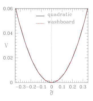
Here $\epsilon$ measures the size of the correction and $\delta$ characterizes the period of oscillation of the correction term in the washboard potential. The reduced potential is shown in the left panel of Fig. 1 for easy visualization. When ${\tilde{\sigma}}\gg\sqrt{\epsilon}$, the potential is almost quadratic. If ${\tilde{\sigma}}\ll\delta$, then $V(\tilde{\sigma})\simeq{1\over 2}(1+{\epsilon/\delta^{2}}){\tilde{\sigma}}^{2}$. Then the curvaton potential is roughly quadratic as well, but has a deformed mass.

The dynamics of curvaton field after inflation is governed by

$${\tilde{\sigma}}^{\prime\prime}+{3\over 2x}{\tilde{\sigma}}^{\prime}+{\tilde{\sigma}}+{\epsilon\over\delta}\sin\left({\tilde{\sigma}/\delta}\right)=0.$$ (22)

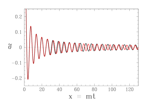
Even though the correction to the potential is small, the dynamics of curvaton field becomes significantly non-linear if the period of the correction term is small enough. Here we consider the case in which the dynamics of curvaton is dominated by the mass term in the beginning, which implies $\epsilon/\delta<1$. Once the amplitude of the curvaton oscillation drops below $\epsilon/\delta$, the curvaton evolves non-linearly. On the right panel of Fig. 1 we have plotted the oscillation of the curvaton field about the minimum of the potential for the quadratic and the washboard potential cases, for the same initial field value given by $\sigma_{*}/M_{p}=0.1$. We can see that the amplitude of oscillation in the washboard case decreases faster than the quadratic case. Moreover, the frequency of oscillation for the washboard curvaton is time dependent, it oscilates about the constant frequency of the quadratic case.

Figure 2: $N_{,\sigma},\ N_{,\sigma\sigma},\ N_{,\sigma\sigma\sigma}$, $f_{NL}$ and $g_{NL}$ are shown as functions of $\epsilon$ for the washboard potential, for fixed values of $\delta,\ \Gamma/m$ and $\sigma_{*}/M_{p}$. We have shown plots for two different values of $\Gamma/m$ in order to demonstrate the systematic variation as we change $\Gamma/m$.

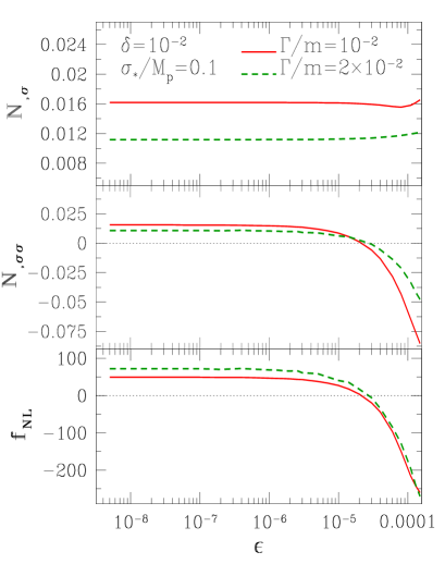
We now illustrate how the small features in the curvaton potential play an important role for the non-Gaussianity parameters. First we solve for $N_{,\sigma}$, $N_{,\sigma\sigma}$ and $N_{,\sigma\sigma\sigma}$ and then obtain $f_{NL}$ and $g_{NL}$ from them. In general, we need to scan four independent parameters, namely, $\Gamma/m,\ \sigma_{*}/M_{p},\ \epsilon$ and $\delta$ in order to satisfy observational constraints such as amplitude of perturbations and the limits on $f_{NL}$ and $g_{NL}$. Our strategy here is to fix $\Gamma/m,\ \sigma_{*}/M_{p}$ and $\delta$ and obtain $f_{NL}$ and $g_{NL}$ as functions of $\epsilon$. Our results are obtained for two values of $\Gamma/m$ and $\delta$ each, to understand how these parameters systematically affect $f_{NL}$ and $g_{NL}$.

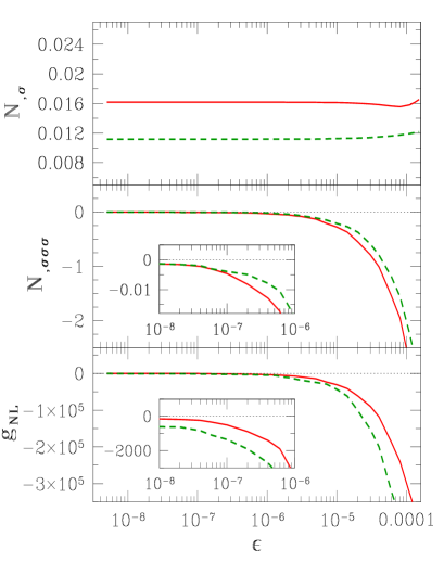
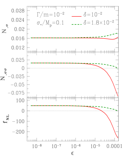
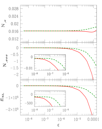
In the case of the quadratic potential $\Gamma/m$ is typically required to be of the order of $10^{-8}$ for the amplitude of perturbations to be COBE normalized. Evolving the equations numerically till the energy density of the curvaton decreases to such small value is prohibitively time consuming. Moreover, for the purpose of capturing the essential features of the dependence of $f_{NL}$ and $g_{NL}$ on $\epsilon$ and $\delta$, it is enough to fix $\Gamma/m$ at a relatively larger value. To demonstrate this point, in Fig. 2 we have plotted for $\Gamma/m=10^{-2}$ and $2\times 10^{-2}$, how $N_{\sigma},\ N_{\sigma\sigma},\ N_{\sigma\sigma\sigma}$, $f_{NL}$ and $g_{NL}$ vary as functions of $\epsilon$, for fixed values of $\delta=10^{-2}$ and $\sigma_{*}/M_{p}=0.1$. We can see that $\Gamma/m$ systematically changes the amplitudes of $f_{NL}$ and $g_{NL}$, but does not alter the essential functional shapes. The correctness of the numerical calculations are tested by ensuring that in the limit $\epsilon\rightarrow 0$, $f_{NL}$ and $g_{NL}$ tend to their analytically expected values for the quadratic potential, as clearly seen in the figure. As $\epsilon$ increases, $f_{NL}$ and $g_{NL}$ get strongly affected and deviates from their expectation from quadratic potential. $f_{NL}$ crosses over from positive to increasingly negative values as $\epsilon$ increases. On the other hand, $g_{NL}$ remains negative throughout but its magnitude becomes very large as $\epsilon$ increases. The inset figures in the panels showing $N_{\sigma\sigma\sigma}$ and $g_{NL}$ zoom in on the $\epsilon\rightarrow 0$ region to show them approaching the negative values expected from quadratic potential.

Next, in Fig. 3 we have plotted $N_{\sigma},\ N_{\sigma\sigma},\ N_{\sigma\sigma\sigma}$, $f_{NL}$ and $g_{NL}$ as functions of $\epsilon$, for two different values of $\delta$. We have chosen $\delta=10^{-2}$ and $1.8\times 10^{-2}$ and fixed $\Gamma/m=10^{-2}$ and $\sigma_{*}/M_{p}=0.1$. We see that for very small $\epsilon$, varying $\delta$ has little effect on the behavior of $f_{NL}$ and $g_{NL}$. This can be explained by the fact that $\epsilon\rightarrow 0$ kills off the oscillations superimposed on the potential, regardless of the frequency of oscillations which is controlled by $\delta$. At relatively larger values of $\epsilon$, the effect of $\delta$ becomes prominent. As the deviation of $f_{NL}$ and $g_{NL}$ from the quadratic potential behavior increases as $\delta$ decreases, due to the increase in the frequency of the oscillations in the potential. As in Fig. 2 the inset figures in the panels showing $N_{\sigma\sigma\sigma}$ and $g_{NL}$ zoom in on the $\epsilon\rightarrow 0$ region to show them approaching the negative values expected from quadratic potential.

Figure 3: Same as Fig. 2 but for two different values of $\delta$, with $\Gamma/m$ and $\sigma_{*}/M_{p}$ kept fixed.

3.2 Single-feature curvaton model

In this subsection we consider a curvaton model with the potential given by

$$V(\sigma)={1\over 2}m^{2}\sigma^{2}\left(1+{c\over 1+(\sigma/M)^{2n}}\right),$$ (23)

where $n>0$, and $M$ is an energy scale which measures the position of the feature. In the regime $\sigma\gg M$ or $\sigma\ll M$, the curvaton potential has a quadratic form, but around $\sigma\sim M$ the potential deviates from quadratic form. As in the previous subsection, we define a reduced potential, as follows

$$V({\tilde{\sigma}})={1\over 2}{\tilde{\sigma}}^{2}\left(1+{c\over 1+({\tilde{\sigma}}/d)^{2n}}\right),$$ (24)

where

$$d={M\over\sigma_{*}}.$$ (25)

Figure 4: The single feature curvaton potential given by Eq. (3.7) is shown on the left panel for comparision with the corresponding quadratic one. $d$ is fixed to be $0.1$ and we have plotted for $c=2$ and $-1$ to show how the nature of the feature changes with the sign of $c$. The right panel shows the corresponding curvaton oscillations about the potential minimum, with the same initial field value given by $\sigma_{*}/M_{p}=0.1$.

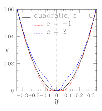
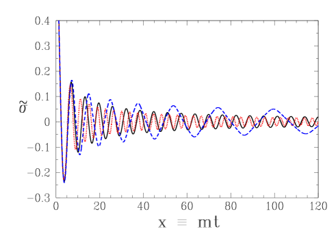
The reduced potential given by Eq. (24) is shown in Fig. 4 for $n=2$ and $d=0.1$. The nature of the feature depends on the sign of $c$. If $c$ is positive, then there is a bump, whereas, a negative $c$ changes the slope of the potential to make it flatter around some scale set by the parameter $d$.

The equation of motion for the reduced curvaton field becomes

$${\tilde{\sigma}}^{\prime\prime} + 3N^{\prime}{\tilde{\sigma}}^{\prime}+\left(1+c{1-(n-1)({\tilde{\sigma}}/d)^{2n}\over(1+({\tilde{\sigma}}/d)^{2n})^{2}}\right){\tilde{\sigma}}=0.$$ (26)

We restrict our analysis here to $n=2$. If $d\ll 1$ and the initial curvaton field value is large enough, then the curvaton evolves linearly prior to its oscillation. We choose $d=0.1$. As in the washboard curvaton model, we choose $\Gamma_{\sigma}/m$ to be $10^{-2}$ and $\sigma_{*}/M_{p}=10^{-1}$. Then we solve for $f_{NL}$, scanning the parameter $c$.

Figure 5: $N_{,\sigma},\ N_{,\sigma\sigma},\ N_{,\sigma\sigma\sigma}$, $f_{NL}$ and $g_{NL}$ are shown as functions of $c$ for the single-feature potential, with $d,\ \Gamma/m$ and $\sigma_{*}/M_{p}$ kept fixed.

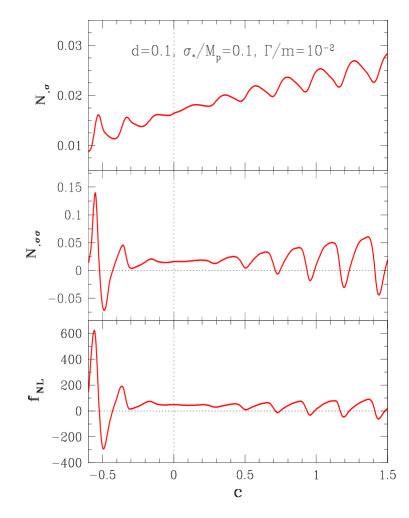
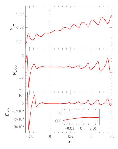
On the left panel of Fig. 5, we have plotted $N_{,\sigma}$, $N_{,\sigma\sigma}$ and $f_{NL}$ for the single-feature potential. As shown in the figure, $f_{NL}$ oscillates about zero with increasing amplitude as $\lvert c\rvert$ increases. We can see $f_{NL}$ flattening out and approaching the expected value from the quadratic potential as $\lvert c\rvert\rightarrow 0$. On the right panel of the same fugure we have plotted $N_{,\sigma}$, $N_{,\sigma\sigma\sigma}$ and $g_{NL}$. We again obtain oscillatory behavior of $g_{NL}$ as $c$ varies. Similar to $f_{NL}$, we can see the curve flattening out near $c=0$ for $g_{NL}$ to assumes the value expected from quadratic potential, as shown in the inset figure on the right bottom panel.

4 Conclusion and discussion

We have studied two new curvaton models in this paper. The first is the washboard model where the potential has tiny oscillations superimposed on the quadratic form, and the second one has a potential with two quadratic regimes having different mass scales separated by either a bump or a flattening of the potential. For the washboard model we have investigated in detail how the two parameters that control the oscillations, namely, the amplitude and the frequency, affect the non-linear corrections to the curvature perturbation via their effect on $f_{NL}$ and $g_{NL}$. We have shown that the relation $g_{NL}\propto-f_{NL}$, which holds for the quadratic potential, is no longer valid in this case. We also found that there is a wide range of both positive and negative values for $f_{NL}$, while $g_{NL}$ remains negative but its magnitude can be very large depending on the model parameters. In comparision, the quadratic potential restricts $f_{NL}$ to be positive and $g_{NL}$ to be negative. For the single-feature model we have again calculated $f_{NL}$ and $g_{NL}$, and demonstrated that they strongly depend on the strength of the feature and oscillate as the strength increases.

What is new in the models considered here is that the curvation motion as it oscillates about the potential minimum is non-linear, unlike other models that have been considered so far in the literature. The results that we have found have interesting implications for searches for non-Gaussianity in observational data. The fact that $f_{NL}$ can switch sign at some parameter values implies that it is possible that the non-linear contributions to the curvature perturbation could be coming from $g_{NL}$ alone, with $f_{NL}$ being close to zero. Similar result was obtained in [14] in the context of curvaton potential with non-linear corrections to the quadratic term. It is also possible that both $f_{NL}$ and $g_{NL}$ contribute comparably with the same or opposite signs. The present work thus throws up the need to understand different sources of primordial non-Gaussianity and how they can be distinguished in the observational data. It is important to devise observables which can distinguish them. Such studies have been initiated in [34, 35]. We also want to mention that $f_{NL}$ and $g_{NL}$ are controlled by two independent geometric quantities which characterize the hyper-surface in field space on which multi-field inflation ends. This has the implication that all of the possible results for $f_{NL}$ and $g_{NL}$ in curvaton models can be realized by tuning these two independent geometric quantities, as shown in [36, 37, 38].

In principle, the three free parameters in the washboard model, $\Gamma/m,\epsilon$ and $\delta$, can be constrained by using the observational constraints on $f_{NL}$, $g_{NL}$ and the amplitude of perturbations. The parameters $c$ and $d$ in the single-feature model can be similarly constrained. However, such a full scan of the parameter space is beyond the scope of the present analysis. Our purpose in this paper has been to understand the systematic behaviors of $f_{NL}$ and $g_{NL}$ as functions of the model parameters. We will tackle the problem of scanning the parameter space in a future work.

Acknowledgments

P.C. is supported by the National Research Foundation of Korea(NRF) grant funded by the Korea government(MEST) (No. 2009-0062868). QGH is supported by the project of Knowledge Innovation Program of Chinese Academy of Science. The numerical calculation in this work was carried out on the QUEST cluster computing facility at Korea Institute for Advanced Study.

Appendix A Curvaton model with quadratic potential

For the curvaton model with quadratic potential, from [33], we have

$$f_{NL} = {5\over 4f_{D}}-{5\over 3}-{5\over 6}f_{D},$$ (27)

$$g_{NL} = -{25\over 6f_{D}}+{25\over 108}+{125\over 27}f_{D}+{25\over 18}f_{D}^{2},$$ (28)

where

$$f_{D}={3\Omega_{\sigma,D}\over 4-\Omega_{\sigma,D}}.$$ (29)

After inflation the universe is dominated by radiation and the Hubble parameter is related to the cosmic time $t$ by $H={1\over 2t}$. The equation of motion of curvaton field with quadratic potential becomes

$${\tilde{\sigma}}^{\prime\prime}+{3\over 2x}{\tilde{\sigma}}^{\prime}+{\tilde{\sigma}}=0,$$ (30)

whose solution is

$${\tilde{\sigma}}=2^{1/4}\Gamma(5/4)x^{-1/4}J_{1/4}(x),$$ (31)

where $J_{\nu}(x)$ is the Bessel function of the first kind. Therefore the energy density of curvaton is given by

$$\rho_{\sigma}={1\over 2}m^{2}\sigma_{*}^{2}\left({\tilde{\sigma}}^{2}+({d{\tilde{\sigma}}\over dx})^{2}\right)={\Gamma^{2}(5/4)\over\sqrt{2}}m^{2}\sigma_{*}^{2}x^{-1/2}\left(J_{1/4}^{2}(x)+J_{5/4}^{2}(x)\right).$$ (32)

Adopting the sudden decay approximation, we have

$$\Omega_{\sigma,D}={\rho_{\sigma}(x_{D})\over 3M_{p}^{2}\Gamma_{\sigma}^{2}}\simeq 0.35{\sigma_{*}^{2}\over M_{p}^{2}}\sqrt{m\over\Gamma_{\sigma}},$$ (33)

in the limit of $x_{D}={1\over 2}{m\over\Gamma_{\sigma}}\gg 1$. In the literatures, $\Omega_{\sigma,D}={\sigma_{*}^{2}\over 6M_{p}^{2}}\sqrt{m\over\Gamma_{\sigma}}$ which is roughly half of our exact retult.

References

- [1] A. H. Guth, “The Inflationary Universe: A Possible Solution To The Horizon And Flatness Problems,” Phys. Rev. D 23, 347 (1981).
- [2] A. H. Guth and S. Y. Pi, “Fluctuations In The New Inflationary Universe,” Phys. Rev. Lett. 49, 1110 (1982).
- [3] K. Enqvist and M. S. Sloth, “Adiabatic CMB perturbations in pre big bang string cosmology,” Nucl. Phys. B 626, 395 (2002) [arXiv:hep-ph/0109214].
- [4] D. H. Lyth and D. Wands, “Generating the curvature perturbation without an inflaton,” Phys. Lett. B 524, 5 (2002) [arXiv:hep-ph/0110002].
- [5] T. Moroi and T. Takahashi, “Effects of cosmological moduli fields on cosmic microwave background,” Phys. Lett. B 522, 215 (2001) [Erratum-ibid. B 539, 303 (2002)] [arXiv:hep-ph/0110096].
- [6] E. Komatsu et al., “Seven-Year Wilkinson Microwave Anisotropy Probe (WMAP) Observations: Cosmological Interpretation,” arXiv:1001.4538 [astro-ph.CO].
- [7] V. Desjacques and U. Seljak, “Signature of primordial non-Gaussianity of -type in the mass function and bias of dark matter haloes,” Phys. Rev. D 81, 023006 (2010) [arXiv:0907.2257 [astro-ph.CO]].
- [8] J. Smidt, A. Amblard, A. Cooray, A. Heavens, D. Munshi and P. Serra, “A Measurement of Cubic-Order Primordial Non-Gaussianity ( and ) With WMAP 5-Year Data,” arXiv:1001.5026 [astro-ph.CO].
- [9] Q. G. Huang, “Large Non-Gaussianity Implication for Curvaton Scenario,” Phys. Lett. B 669, 260 (2008) [arXiv:0801.0467 [hep-th]].
- [10] Q. G. Huang, “A Curvaton with a Polynomial Potential,” JCAP 0811, 005 (2008) [arXiv:0808.1793 [hep-th]].
- [11] K. Enqvist, S. Nurmi, G. Rigopoulos, O. Taanila and T. Takahashi, “The Subdominant Curvaton,” JCAP 0911, 003 (2009) [arXiv:0906.3126 [astro-ph.CO]].
- [12] K. Enqvist and T. Takahashi, “Effect of Background Evolution on the Curvaton Non-Gaussianity,” JCAP 0912, 001 (2009) [arXiv:0909.5362 [astro-ph.CO]].
- [13] K. Enqvist, S. Nurmi, O. Taanila and T. Takahashi, “Non-Gaussian Fingerprints of Self-Interacting Curvaton,” JCAP 1004, 009 (2010) [arXiv:0912.4657 [astro-ph.CO]].
- [14] K. Enqvist and S. Nurmi, “Non-gaussianity in curvaton models with nearly quadratic potential,” JCAP 0510, 013 (2005) [arXiv:astro-ph/0508573].
- [15] M. Sasaki, J. Valiviita and D. Wands, “Non-gaussianity of the primordial perturbation in the curvaton model,” Phys. Rev. D 74, 103003 (2006) [arXiv:astro-ph/0607627].
- [16] K. Enqvist and T. Takahashi, “Signatures of Non-Gaussianity in the Curvaton Model,” JCAP 0809, 012 (2008) [arXiv:0807.3069 [astro-ph]].
- [17] Q. G. Huang and Y. Wang, “Curvaton Dynamics and the Non-Linearity Parameters in Curvaton Model,” JCAP 0809, 025 (2008) [arXiv:0808.1168 [hep-th]].
- [18] M. Kawasaki, K. Nakayama and F. Takahashi, “Hilltop Non-Gaussianity,” JCAP 0901, 026 (2009) [arXiv:0810.1585 [hep-ph]].
- [19] P. Chingangbam and Q. G. Huang, “The Curvature Perturbation in the Axion-type Curvaton Model,” JCAP 0904, 031 (2009) [arXiv:0902.2619 [astro-ph.CO]].
- [20] H. Assadullahi, J. Valiviita and D. Wands, “Primordial non-Gaussianity from two curvaton decays,” Phys. Rev. D 76, 103003 (2007) [arXiv:0708.0223 [hep-ph]].
- [21] Q. G. Huang, “The N-vaton,” JCAP 0809, 017 (2008) [arXiv:0807.1567 [hep-th]].
- [22] C. T. Byrnes, S. Nurmi, G. Tasinato and D. Wands, “Scale dependence of local ,” JCAP 1002, 034 (2010) [arXiv:0911.2780 [astro-ph.CO]].
- [23] E. Kawakami, M. Kawasaki, K. Nakayama and F. Takahashi, “Non-Gaussianity from Isocurvature Perturbations : Analysis of Trispectrum,” JCAP 0909, 002 (2009) [arXiv:0905.1552 [astro-ph.CO]].
- [24] T. Matsuda, “Delta-N formalism for the evolution of the curvature perturbations in generalized multi-field inflation,” Phys. Lett. B 682, 163 (2009) [arXiv:0906.2525 [hep-th]].
- [25] T. Takahashi, M. Yamaguchi and S. Yokoyama, “Primordial Non-Gaussianity in Models with Dark Matter Isocurvature Fluctuations,” Phys. Rev. D 80, 063524 (2009) [arXiv:0907.3052 [astro-ph.CO]].
- [26] K. Nakayama and J. Yokoyama, “Gravitational Wave Background and Non-Gaussianity as a Probe of the Curvaton Scenario,” JCAP 1001, 010 (2010) [arXiv:0910.0715 [astro-ph.CO]].
- [27] M. Kawasaki, T. Takahashi and S. Yokoyama, “Density Fluctuations in Thermal Inflation and Non-Gaussianity,” JCAP 0912, 012 (2009) [arXiv:0910.3053 [hep-th]].
- [28] Y. F. Cai and Y. Wang, “Large Nonlocal Non-Gaussianity from a Curvaton Brane,” arXiv:1005.0127 [hep-th].
- [29] A. A. Starobinsky, “Multicomponent de Sitter (Inflationary) Stages and the Generation of Perturbations,” JETP Lett. 42 (1985) 152.
- [30] M. Sasaki and E. D. Stewart, “A General Analytic Formula For The Spectral Index Of The Density Perturbations Produced During Inflation,” Prog. Theor. Phys. 95, 71 (1996) [arXiv:astro-ph/9507001].
- [31] M. Sasaki and T. Tanaka, “Super-horizon scale dynamics of multi-scalar inflation,” Prog. Theor. Phys. 99, 763 (1998) [arXiv:gr-qc/9801017].
- [32] D. H. Lyth, K. A. Malik and M. Sasaki, “A general proof of the conservation of the curvature perturbation,” JCAP 0505, 004 (2005) [arXiv:astro-ph/0411220].
- [33] D. H. Lyth and Y. Rodriguez, “The inflationary prediction for primordial non-gaussianity,” Phys. Rev. Lett. 95, 121302 (2005) [arXiv:astro-ph/0504045].
- [34] P. Chingangbam and C. Park, “Statistical nature of non-Gaussianity from cubic order primordial perturbations: CMB map simulations and genus statistic,” JCAP 0912, 019 (2009) [arXiv:0908.1696 [astro-ph.CO]].
- [35] T. Matsubara, “Analytic Minkowski Functionals of the Cosmic Microwave Background: Second-order Non-Gaussianity with Bispectrum and Trispectrum,” Phys. Rev. D 81, 083505 (2010) [arXiv:1001.2321 [astro-ph.CO]].
- [36] Q. G. Huang, “A geometric description of the non-Gaussianity generated at the end of multi-field inflation,” JCAP 0906, 035 (2009) [arXiv:0904.2649 [hep-th]].
- [37] M. Sasaki, “Multi-brid inflation and non-Gaussianity,” Prog. Theor. Phys. 120, 159 (2008) [arXiv:0805.0974 [astro-ph]].
- [38] Q. G. Huang, “The Trispectrum in the Multi-brid Inflation,” JCAP 0905, 005 (2009) [arXiv:0903.1542 [hep-th]].