Dynamic relaxation of a liquid cavity under amorphous boundary conditions

Abstract

The growth of cooperatively rearranging regions was invoked long ago by Adam and Gibbs to explain the slowing down of glass-forming liquids. The lack of knowledge about the nature of the growing order, though, complicates the definition of an appropriate correlation function. One option is the point-to-set correlation function, which measures the spatial span of the influence of amorphous boundary conditions on a confined system. By using a swap Montecarlo algorithm we measure the equilibration time of a liquid droplet bounded by amorphous boundary conditions in a model glass-former at low temperature, and we show that the cavity relaxation time increases with the size of the droplet, saturating to the bulk value when the droplet outgrows the point-to-set correlation length. This fact supports the idea that the point-to-set correlation length is the natural size of the cooperatively rearranging regions. On the other hand, the cavity relaxation time computed by a standard, nonswap dynamics, has the opposite behavior, showing a very steep increase when the cavity size is decreased. We try to reconcile this difference by discussing the possible hybridization between MCT and activated processes, and by introducing a new kind of amorphous boundary conditions, inspired by the concept of frozen external state as an alternative to the commonly used frozen external configuration.

I Introduction

It is common wisdom that the spectacular slowing down of supercooled liquids at low temperature is caused by the growth of a correlation length of some sort. The underlying idea is that of cooperativity: at lower temperatures, larger regions (termed cooperatively rearranging regions) must move together in order to fully relax Adam and Gibbs (1965). Unfortunately, the standard tools used in critical phenomena to detect a growing correlation length fail in glass-forming liquids, as it is not at all clear a priori what the order parameter should be. No obvious domain or structure can be observed in a low temperature liquid to distinguish it from a high temperature one. If order is growing in glass-formers, it must be some sort of amorphous order, and the corresponding order parameter must be nonstandard.

Recently, some progress has been achieved by using amorphous boundary conditions (ABC) Bouchaud and Biroli (2004); Cavagna et al. (2007); Biroli et al. (2008). The idea goes as follows Bouchaud and Biroli (2004). Consider a low-temperature equilibrium configuration of a liquid and freeze all particles outside a certain region. This region (or cavity) is then let free to evolve and thermalize, subject to the pinning field produced by all the frozen particles surrounding it. Clearly, the smaller the region the stronger the effect of the pinning field, hence keeping the region in a very restricted portion of its own phase space. The idea, then, is to check how large the region must be to emancipate from the boundary conditions, i.e. to regain ergodicity and thermalize into a state different from the surrounding one. The advantage of this method is that the system chooses its own definition of ‘order’ by means of the amorphous boundary conditions, and we do not need to have any a priori knowledge of the nature of such order. Practically speaking, the procedure amounts to measure, as a function of the size $R$ of the region, the correlation between the original region’s configuration (that of the frozen surrounding) and that achieved after the region has equilibrated subject to the amorphous boundary conditions. This quantity is called point-to-set correlation function Mézard and Montanari (2006); Montanari and Semerjian (2006), $q(R)$, and it has shown an interesting feature Cavagna et al. (2007); Biroli et al. (2008): its decay length-scale, $\xi_{s}$, increases on lowering $T$. Regions smaller than $\xi_{s}$ cannot relax completely, even given infinite time, due to the presence of the pinning ABC.

Here, in order to get some information about the dynamics of the cooperatively rearranging regions, we study the dynamical behavior of a cavity under ABC. Of course, we do expect that the equilibration time of the cavity must be equal to its bulk value for large enough values of $R$. What is not trivial is at what specific value of $R$ the saturation occurs and whether the saturation occurs from above or from below, i.e. whether the equilibration time decreases or increases when the cavity gets larger. As we shall see, we obtain different results according to the specific dynamics we use: by means of a swap Montecarlo dynamics, where particles of different species can be exchanged in order to accelerate the dynamics, we find a clear saturation from below of the equilibration time taking place at $R\sim\xi_{s}$ (Section III). This result seems to support the idea that $\xi_{s}$ is indeed the cooperativity length scale of the system (Sections IV– VI). If, on the other hand, we use a standard, nonswap algorithm, we find that the dynamics slows down very steeply when the cavity size is decreased (Section VII).

We will discuss the meaning of these results and how this difference may be related to the actual relaxation mechanism active for the cooperatively rearranging regions in the bulk. In particular, we will show that the hybridization between the Mode Coupling Theory (MCT) and the activated relaxation channels can give rise to a nonmonotonic behavior of the relaxation time as a function of the cavity radius (Section VIII). We will also put forward the hypothesis that the standard amorphous boundary conditions, where the external configuration is frozen, introduce an artificial slowing down of the cavity dynamics, which can be overcome by switching to the more physical frozen state boundary conditions (Sections IX– X). After briefly commenting on some relevant experiments (Section XI) we summarize our conclusions in Section XII.

II Model and observables

We perform Monte Carlo (MC) simulations of a 3-$d$ soft-spheres binary mixture Bernu et al. (1987) with parameters as in Ref. Biroli et al. (2008). The mode-coupling temperature Götze and Sjorgen (1992) for this system is $T_{MC}=0.226$ Roux et al. (1989). Our largest system has $N=16384$ particles in a box of length $L=25.4$. We run simulations at $T=0.482,0.350,0.246,0.214,0.202$. We first equilibrate the whole system with periodic boundary conditions to generate a set of equilibrium configurations, and then run the amorphous boundary simulations by picking an equilibrium configuration and artificially freezing all particles but those occupying a spherical cavity of radius $R=$ 1.06, 1.68, 1.92, 2.12, 2.28, 2.61, 2.87, 3.29, 3.62, 4.15, 4.57, 5.75, 7.2, 9.14, and 10.95. We use at least 16 samples for each $T$ and $R$.

Our main physical observable is the overlap, which measures the correlation between the running configuration and the reference one at $t=0$. The cavity is partitioned in small cubic boxes and $n_{i}$ is the number of particles in box $i$. The side $\ell$ of the cells is such that $n_{i}=\{0,1\}$. We measure the overlap within a small cubic volume $v$ located at the center of the sphere Biroli et al. (2008),

$$q(t;R)\equiv\frac{1}{\ell^{3}\,N_{i}}\sum_{i\in v}n_{i}(t)\,n_{i}(0)\ ,$$ (1)

where the sum runs over all boxes and $N_{i}$ is the number of boxes in the central volume. To minimize statistical uncertainty without losing the local nature we choose $N_{i}=v/\ell^{3}=125$. On average, the overlap of two identical configurations is $1$, while for totally uncorrelated configurations $q=q_{0}=\ell^{3}=0.062876$. The asymptotic value of the overlap, $q(R)\equiv\langle q(t\to\infty;R)\rangle$, averaged over many realizations of the boundary conditions, is the point-to-set correlation function Bouchaud and Biroli (2004); Montanari and Semerjian (2006); Cavagna et al. (2007); Biroli et al. (2008); Biroli and Bouchaud (2009).

In order to define a time-scale we measure the connected auto-correlation function of the overlap fluctuations,

$$C(t;R)=\frac{\left\langle\left(q(t_{0}+t;R)-q(R)\right)\left(q(t_{0};R)-q(R)\right)\right\rangle}{\left\langle\left(q(t_{0};R)-q(R)\right)^{2}\right\rangle}\ .$$ (2)

To estimate the equilibration time $\tau(R)$ we use the method discussed by A. Sokal in Sokal (1997), based on the integral of the correlation function. More specifically, the relaxation time $\tau$ is found by solving the equation,

$$\tau=\int_{0}^{\alpha\tau}dt\ C(t;R)\ ,$$ (3)

where the optimal value of $\alpha$ has been found to be $20$. In this way one is sure to sample the phenomenon on a time window that is self consistently much larger than the relaxation time.

III Swap dynamics in the confined cavity

Figure 1: Autocorrelation function $C(t;R)$ for a few representative sizes $R$ at $T=0.202$.

We first focus on the results obtained with swap dynamics Grigera and Parisi (2001). With a swap Monte Carlo dynamics we propose (with probability 0.1) a move that swaps the position of two different particles. Provided that the radii of the two different species are not too different, so that the swap move is not always rejected, this kind of move decreases significantly the time needed by a single particle to break its cage. On the other hand, the swap dynamics has less of an impact on collective rearrangements, and indeed the swap relaxation time increases dramatically close to the glass transition, as the nonswap time.

Fig. 1 shows the swap auto-correlation function $C(t;R)$ at various values of $R$ for our lowest temperature $T=0.202$. We stress that for those values of $R$ such that the order parameter $q(R)\neq 0$, ergodicity is broken Biroli et al. (2008). In this case the connected correlation function (2) describes the equilibrium dynamics within a restricted region of the cavity’s phase space.

Before estimating the relaxation time it is very important to be sure that the autocorrelation function does not depend on the size of the time window $\Delta t$ used to measure it. To this aim in Fig. 2 we show the autocorrelation function at our lowest temperature and at different values of the time window $\Delta t$, at two values of $R$: there is no significant dependence of $C(t;R)$ on $\Delta t$.

Figure 2: Test of thermalization of the autocorrelation function. We have computed $C(t,R)$ using increasingly longer time windows, to be sure that the autocorrelation function was saturated. Neither for large or small $R$ is there evidence of any residual dependence on the time window. $T=0.202$.

In Fig. 3 we report the swap equilibration time $\tau(R)$ for our lowest temperature, $T=0.202$. Three features of this curve stand out: i) the swap equilibration time saturates for large $R$ to a value independent of the cavity size; ii) the swap equilibration time grows with $R$, so that saturation occurs from below; iii) growth and saturation are separated by a rather sharp kink at a well-defined value of $R$. The first fact is obvious: the effect of the boundary conditions is expected to fade away for large $R$, so that $\tau(R)$ must eventually reach its bulk value, which is exactly what happens. The remarkable point is that $\tau(R)$ reaches its bulk value for $R\sim\xi_{s}$, where $\xi_{s}$ is the point-to-set correlation length measured in Ref. Biroli et al. (2008).

This result can immediately be interpreted in terms of cooperativity: For $R<\xi_{s}$ the whole region is correlated, because the effect of the amorphous border breaks the ergodicity. For $R>\xi_{s}$, the effect of the border fades away and the region is able to decorrelate by breaking up into smaller correlated sub-parts: in this regime relaxation factorizes. Hence, it seems that the point-to-set correlation length $\xi_{s}$ does indeed play a role in the cooperative dynamics of the system. In the next Sections we will address this point more precisely.

Figure 3: Cavity relaxation time vs. $R$ for $T=0.202$. The kink between the growth and the saturated regime occurs close to $\xi_{s}=3.82\pm 0.46$, which is the point-to-set lengthscale for $T=0.202$ Biroli et al. (2008). Also shown is the bulk (periodic boundary conditions) equilibration time (full line).

IV RFOT interpretation of the swap equilibration time

According to the random first-order theory (RFOT) of the glass transition, whether or not a region of radius $R$ relaxes depends on the balance between the surface tension $Y$ that develops when that region actually rearranges and the configurational entropy $\Sigma$ unleashed by the rearrangement: if $Y>T\Sigma R^{d-\theta}$ ($d$ is the space dimension, $\theta$ is the surface tension —or stiffness— exponent) the surface cost is larger than the entropic gain and the region does not rearrange. On the other hand, if $Y<T\Sigma R^{d-\theta}$ the entropic gain outweighs the surface energy cost and the region has a thermodynamic advantage to rearrange. The rearranging size where entropy and surface tension balance, $\xi_{s}=\left(Y/T\Sigma\right)^{1/(d-\theta)}$, is the static correlation length of RFOT.

Therefore, within RFOT a cavity with amorphous boundary conditions of radius $R<\xi_{s}$ has broken ergodicity, and can only explore the state imposed by the boundary conditions Bouchaud and Biroli (2004). In this regime the equilibration time is the time needed to explore that one state, which is roughly equal to the $\beta$-relaxation time, $\tau(R)\sim\tau_{\beta}$ . For $R>\xi_{s}$, instead, rearrangement occurs and ergodicity of the cavity is restored. In this regime the region is larger than the minimal rearranging size, so that relaxation factorizes: different subregions of size $\xi_{s}$ will rearrange independently from each other, and the equilibration time will be equal to its bulk value, i.e. $\tau(R)\sim\tau_{0}\exp(\xi_{s}^{\psi}/T)$, where $\tau_{0}$ is an Arrhenius prefactor and $\psi$ is the exponent regulating the barrier growth.

Hence, within the sharp RFOT description, where the surface tension has just one value, $Y$, it is predicted a step-like jump of $\tau(R)$ at $R=\xi_{s}$, from $\tau_{\beta}$ up to $\tau_{0}\exp(\xi_{s}^{\psi}/T)$,

$$\tau(R)\sim\begin{cases}\tau_{\beta}&R<\xi_{s}\\ \tau_{0}\,e^{\xi_{s}^{\psi}/T}&R>\xi_{s}\ .\end{cases}$$ (4)

Such stepwise behavior is not what we observed in Fig. 3. In order to reconcile data and theory, we note that for the typical temperatures and sizes studied in simulations surface tension fluctuations are relevant Biroli et al. (2008). If the surface tension fluctuates (i.e. different ABCs give different $Y$), local excitations can have different sizes and therefore different relaxation times. When we measure these quantities by averaging over many different sets of ABC we smooth out the sharp behavior of (4).

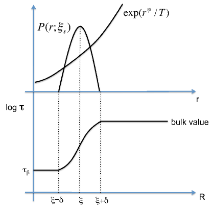
Figure 4: Schematic view of the second integral in equation (7). The upper panel represents the two functions within the integral, the lower panel is the resulting relaxation time.

To see more precisely how this happens, let us write the surface tension distribution as $P(Y;Y_{c})$, where now $Y$ is the fluctuating surface tension, whereas $Y_{c}$ is its typical scale, defined by the peak of the distribution. This means that a region of radius $R$ will rearrange or not rearrange, depending on the value of $Y$; accordingly, its relaxation time can be the either the in-state time $\tau_{\beta}$, or the time needed to activately rearrange the region,

$$\tau(R,Y)\sim\begin{cases}\tau_{\beta}&Y>T\Sigma R^{d-\theta}\\ \tau_{0}\,\exp\left[\frac{1}{T}\left(Y/T\Sigma\right)^{\frac{\psi}{d-\theta}}\right]&Y<T\Sigma R^{d-\theta}.\end{cases}$$ (5)

The macrosopic equilibration time will be given by an average over $Y$ of the time in (5),

$$\begin{split}\tau(R)&=\tau_{\beta}\int_{T\Sigma R^{d-\theta}}^{\infty}P(Y;Y_{c})\,dY\ +\\ +\ &\quad\tau_{0}\int_{0}^{T\Sigma R^{d-\theta}}P(Y;Y_{c})\;\exp\left[\frac{1}{T}\left(Y/T\Sigma\right)^{\frac{\psi}{d-\theta}}\right]\,dY.\end{split}$$ (6)

The first term in (6) corresponds to regions surrounded by large surface tension, which do not rearrange, and it equals at most $\tau_{\beta}$. The second term corresponds to the low surface tension regions that do rearrange, and at low temperatures this term is large. Clearly, if $P(Y;Y_{c})=\delta(Y-Y_{c})$ we recover the step-like behavior of $\tau(R)$ described in (4). If, on the other hand, $P(Y;Y_{c})$ is broad, the result is nontrivial.

With a fluctuating surface tension we can still define a typical mosaic correlation length, $\xi_{s}=\left(Y_{c}/T\Sigma\right)^{1/(d-\theta)}$ Biroli et al. (2008). This relation suggests an obvious change of variables useful to recast equation (6) in a simpler form:

$$\tau(R)=\tau_{\beta}\int_{R}^{\infty}P(r;\xi_{s})\,dr+\tau_{0}\int_{0}^{R}P(r;\xi_{s})\;e^{r^{\psi}/T}\,dr,$$ (7)

where we are now integrating over all possible sizes of the rearranging regions. $P(r;\xi_{s})$ is the distribution of sizes, which is of course peaked on $\xi_{s}$. To understand the behavior of the function $\tau(R)$ let us assume that $P(r;\xi_{s})$ has a compact support, being different from zero only in the interval $r\in[\xi_{s}-\delta:\xi_{s}+\delta]$, and zero elsewhere. We have three regimes of $R$ (see Fig. 4):

i) for $R<\xi_{s}-\delta$ the first integral in (7) is $1$ and the second integral is $0$, so that $\tau(R)=\tau_{\beta}$;

ii) for $\xi_{s}-\delta<R<\xi_{s}+\delta$ the weight shifts from the first to the second integral; because of the exponential, which is large at low $T$, $\tau$ grows with growing $R$, thus giving rise to a ramp that brings the relaxation time to a value considerably larger than $\tau_{\beta}$;

iii) for $R>\xi_{s}+\delta$, the first integral is $0$, whereas the second one has reached its saturation value; to know this value, at low $T$ we can use the saddle point approximation: the maximum of the integrand occurs approximately for $r\sim\xi_{s}$, so that $\tau(R)\sim\tau_{0}\ e^{\xi_{s}^{\psi}/T}$. This last quantity is nothing else than the bulk relaxation time, $\tau_{\mathrm{bulk}}$.

Figure 5: Cavity relaxation time $\tau(R)$, normalized to its bulk value, at various $T$. From right to left: $T=0.202,0.246,0.350,0.482$. The saturation length scale of $\tau(R)$, reported in the next figure, is defined by the crossing of the large $R$ (bulk) value of $\tau$ and the linear fit (in semi-log) of the small $R$ data. This method is straightforward at lower $T$, where $\tau(R)$ is unambiguously monotonic, but less so at higher $T$, where a small overshooting exists. We will discuss the origin of this overshooting in the following Sections.

What we have just described is a smooth growth of $\tau(R)$ from $\tau_{\beta}$ up to the bulk relaxation time $\tau_{\mathrm{bulk}}$, taking place in a range of $R$ around $\xi_{s}$,

$$\tau(R)\sim\begin{cases}\tau_{\beta}&\text{for $R<\xi_{s}-\delta$}\\ \text{growth}&\text{for $\xi_{s}-\delta<R<\xi_{s}+\delta$}\\ \tau_{0}\;e^{\xi_{s}^{\psi}/T}&\text{for $R>\xi_{s}+\delta$}\ .\end{cases}$$ (8)

It is difficult to better specify the behavior of $\tau(R)$ in its increasing regime with no knowledge of the distribution $P(r;\xi_{s})$ (or, equivalently, of $P(Y;Y_{c})$). Still, in the saddle point limit (low $T$) there is something we can say: the second integral in (7) is dominated by the exponential, and for $R<\xi$ the saddle-point coincides with the right edge of the integration domain, $r_{\mathrm{S}P}=R$. In this case we have,

$$\tau(R)\sim\tau_{0}\ e^{R^{\psi}/T},\qquad\xi_{s}-\delta<R<\xi_{s}+\delta.$$ (9)

The behavior described by (8) is in agreement with what we have found in our swap simulations (Fig. 3). The relaxation time grows with the radius of the cavity, and it saturates to its bulk value at $R\sim\xi_{s}$, so that we can use the saturation point as an estimate of the static correlation length $\xi_{s}$. In Fig. 5 we report the cavity swap relaxation time normalized by its bulk value for several different temperatures. We can see that the saturation point moves to larger values of $R$ at lower temperatures, a phenomenon consistent with the expectation that the correlation length grows when cooling the system. This fact consolidates the idea that the point where the cavity relaxation time saturates is indeed the same static correlation length as extracted from the point-to-set correlation function.

We test this interpretation by plotting in Fig. 6 the length scale of saturation of the swap relaxation time vs. the value of the static correlation length extracted by the point-to-set correlation function computed in Biroli et al. (2008). Considering that both length scales have a degree of arbitrariness in their measurement, we normalize them in order to be equal at one specific temperature (see the caption of Fig. 6). Even though we definitely would need a wider temperature range to say something certain, we can conclude that the two length scales track each other quite reasonably. This supports the idea that the point-to-set correlation length (an eminently static concept) can actually be measured also by using the swap relaxation time of a cavity subject to amorphous boundary conditions.

Figure 6: Comparison between the correlation length extracted from the cavity relaxation time (abscissa) and the point-to-set (PTS) correlation length (ordinate). The PTS correlation length has beed defined as the value of $R$ at which the PTS correlation function crosses a certain value $\eta$. Given the arbitrariness of $\eta$, its value has been chosen in such a way to have the two length scales equal at $T=0.482$.

V When cooler is faster

Both the stepwise behavior of (4) and the smooth growth of (8) have an interesting consequence: at some values of $R$ a colder cavity may be faster than a hotter cavity. How this happens is pictorially explained in Fig. 7. By lowering the temperature, $\xi_{s}$ increases, so we push to the right the support of $P(r;\xi_{s})$, and therefore the range of $R$ over which the growth of $\tau(R)$ occurs; at the same time, the bulk relaxation time increases, so that the low $T$ curve must saturate at a higher level than the high $T$ curve. This mechanism gives rise to a crossing of the cold and hot relaxation times, so that in the region of $R$ between the cold and hot value of $\xi_{s}$, we have that the lower $T$ cavity has a smaller relaxation time than the higher $T$ cavity.

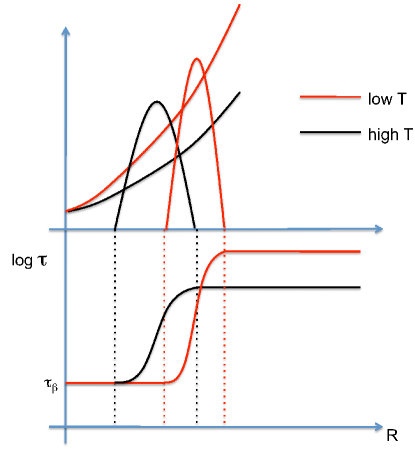
Figure 7: Schematic view showing how an inversion of the cold and hot relaxation times can take place. By lowering the temperature two (related) phenomena occur: i) the correlation length increases, so that the distribution $P(r;\xi_{s})$ moves overall to the right (it also becomes more peaked, see Cammarota et al. (2009a), but this is irrelevant here); ii) the asymptotic bulk relaxation time increases, so at saturation $\tau(R)$ reaches a higher level. These two phenomena give rise to a regime, between the two correlation lengths, where the relaxation time of the colder cavity is lower than that of the hotter cavity.

This odd phenomenon is confirmed by our swap simulations. In Fig. 8 we show the cavity swap relaxation time at two different values of $T$. It can be seen quite clearly that for certain values of the radius the cold cavity is faster than the warm cavity. In the inset of Fig. 8 we directly show the two autocorrelation functions for one specific value of $R$, just to make clear that the effect does not depend on the particular definition of $\tau$.

Figure 8: Swap simulations show that an inversion of the relaxation time indeed happens: there is an intermediate regime of $R\in[1.5,2.5]$ where the low temperature cavity (full circles, $T=0.202$) is faster than the high temperature cavity (open squares, $T=0.350$). Inset: the autocorrelation function at fixed $R=1.68$ at the two different temperatures. Irrespective of the definition of the relaxation time, the cooler cavity is faster.

As we have seen, this interesting phenomenon is quite naturally explained in the context of RFOT. In the sharp scenario, the inversion of cold and warm relaxation times is a direct consequence of the presence of two qualitatively different times: the short in-state time, $\tau_{\beta}$, and the long out-state relaxation time, $\tau_{\mathrm{bulk}}$. The existence of these two times means that at a certain value of $R$ a cold cavity may still be trapped into its original state, therefore having a short in-state relaxation time, whereas a warm cavity may be unlocked, and therefore have a longer relaxation time. We remark, once again, that one is comparing qualitatively different times: the in-state time $\tau_{\beta}$ is the time needed to relax within a state, with no cooperative rearrangement, while the relaxation time of a large cavity, $\tau_{\mathrm{bulk}}$ is the time needed for a full rearrangement. Such distinction is sharp, and easy to detect, only in the stepwise scenario of equation (4). On the other hand, as we have seen, in the real case $\tau(R)$ (averaged over many samples) is a smooth function, with a ramp connecting the in-state time to the bulk time, so that it is harder to distinguish the two different processes from the full $\tau(R)$ curve. The inversion of cold and hot relaxation times is therefore an interesting remnant of the presence of these two different time scales.

VI An unexpected inequality

In order to have a finite bulk equilibration time, we need the second integral in equation (6) to be finite for $R\to\infty$. Therefore $P(Y;Y_{c})$ must decay sufficiently fast to suppress the Arrhenius factor. If we make the reasonable assumption,

$$P(Y;Y_{c})\sim e^{-(Y/Y_{c})^{\nu}},\qquad Y\gg 1,$$ (10)

we must have,

$$\nu\geq\frac{\psi}{d-\theta}.$$ (11)

As we have seen, the distribution $P(Y;Y_{c})$ implies an equivalent distribution of the rearranging regions’ size, $P(R;\xi_{\rm s})$, inequality (11) means that $P(R;\xi_{s})$ must decay fast enough to suppress the growth of the equilibration times for large $R$. This is reasonable. In Biroli et al. (2008) it was shown that the exponent $\nu$ is related to the anomaly exponent $\zeta$ that rules the nonexponential decay of the point-to-set correlation function $q(R)$,

$$q(R)\sim e^{-(R/\xi_{s})^{\zeta}},$$ (12)

with

$$\zeta=\nu(d-\theta),\qquad\zeta\geq 1.$$ (13)

where $\theta$ is the surface tension (or stiffness) exponent. This leaves us with the inequality,

$$\zeta\geq\psi.$$ (14)

On increasing the temperature the anomaly $\zeta$ must go to $1$, as the point-to-set correlation function $q(R)$ becomes a pure exponential Biroli et al. (2008). If $\psi$ is temperature-independent, relation (14) then implies,

$$\psi\leq 1.$$ (15)

We note that the value $\psi\sim 1$ previously reported in Cammarota et al. (2009b) satisfies (15). Of course, if we allow $\psi$ to depend on $T$ (as $\zeta$ does), then there would be no reason for (15) to be valid in general, whereas (14) would still hold.

VII Nonswap dynamics in the confined cavity

Figure 9: Standard nonswap Monte Carlo dynamics. Connected overlap as a function of time for four different sizes of the cavity. The connected overlap is obtained by subtracting its equilibrium infinite time limit, $q(R)$, obtained with swap, and its asymptotic value must be equal to zero. Smaller sizes are significantly slower than larger sizes. For $R\leq 3.5$ the dynamics is completely stuck. $T=0.246$.

The dynamical behavior of the cavity when we switch off the swap moves is completely different from what we have seen until now: in contrast to the swap case, the relaxation is slower the smaller the cavity. In the bulk, the dynamics without swap is known to be significantly slower than with swap Grigera and Parisi (2001) (this is why swap has been introduced in the first place). However, in the cavity, not only is nonswap dynamics slower, but the whole dynamical behavior as a function of $R$ is reversed.

We observe this phenomenon in Fig. 9, where we report the connected overlap as a function of time in the nonswap case for different values of $R$. The connected overlap is obtained by subtracting from $q(t)$ its equilibrium infinite time limit, $q(R)$, obtained with swap. The asymptotic value of the connected overlap must be equal to zero for all $R$ and this makes it easier to compare different sizes on the same plot. Smaller cavities are dramatically slower than larger ones. Under these conditions, it is clear that we cannot compute the overlap autocorrelation function in the nonswap case, as the system is robustly out of equilibrium. The only time correlation function that we can use is the overlap itself, $q(t)$, and to extract a relaxation time, $\tau(R)$, we cross $q(t)$ with an arbitrary value, $\bar{q}$. For those (few) values of $R$ for which this procedure is viable, we report $\tau(R)$ in Fig. 10.

Figure 10: Standard nonswap Montecarlo dynamics. Relaxation time obtained by crossing the overlap time series in Fig. 9 with the arbitrary value $\bar{q}=0.25$. For smaller values of $R$ the nonswap dynamics is completely stuck, and an extrapolation of $q(t)$ does not make any sense (see Fig. 11).

In smaller cavities, below $R\sim 4$, the nonswap overlap is completely stuck to a level which is above its equilibrium value. We can clearly see this by using a BIC (Beta Initial Condition) test. The idea is to initialize the cavity in a configuration $\beta$ which has overlap equal to zero with the $\alpha$ configuration used to thermalize the system, and which is frozen in the boundary condition. In this way, the BIC overlap $q_{\alpha\beta}(t)$ is zero at time zero, and it must increase to the same asymptotic value as the standard overlap $q_{\alpha\alpha}(t)$. When thermalization of the cavity is achieved the two overlaps must meet at the same equilibrium value, $q(R)$ .

Figure 11: BIC test comparison between swap and nonswap dynamics. In the BIC test the configuration is initialized both in the same configuration $\alpha$ as the frozen boundary (upper, full curve) and in a different configuration $\beta$ with respect to the frozen boundary (lower, dashed curve). The upper and lower curves must reach the same asymptotic value $q(R)$ for infinite times. The BIC test is positive for the swap dynamics; all of our swap data, fore every value of $R$ and $T$, have passed the BIC test. On the other hand, the BIC test is negative for the nonswap dynamics. Nevertheless, the nonswap time series is stationary, making it impossible to estimate a reasonable value of the relaxation time. $R=2.27$, $T=0.246$.

A positive BIC test is shown in the upper panel of Fig. 11 for the swap dynamics at small R: the two overlap branches meet at their asymptotic value, $q(R)$. We have run BIC tests for all our values of $R$ and $T$ in the swap case, always getting a positive result (the same holds for the data of Biroli et al. (2008)). In the lower panel of the same figure we see what happens in the nonswap case for the same value of $R$: despite the fact that the overlap is stationary for several decades, it is definitely not thermalized, as there is a clear and significant gap between the two branches, none of which reaches the equilibrium value $q(R)$ (dotted line). Hence, at this value of $R$ and of $T$ it is not even possible to roughly estimate $\tau$: no extrapolation of $q(T)$, however wild, makes sense with these data.

We notice that this slowing down happens also at relatively high temperatures: the effect of the confinement on the relaxation time is really drastic, and the difference between swap and nonswap dynamics stark. Incidentally, we note that without swap dynamics it would be impossible to measure the point-to-set correlation function (which is the equilibrium value of $q$), due to this hyper-slowing down. The slowing down of the dynamics in a confined cavity was noted before in ref. Berthier and Kob (2011) for molecular dynamics.

In the next Sections we address the conflict between the swap and nonswap results.

VIII The contradiction between swap and nonswap

At this point we are left with a contradictory scenario. On one hand, with swap Monte Carlo the relaxation time grows up to its bulk value when increasing the cavity radius $R$, seemingly saturating when $R$ reaches the point-to-set correlation length $\xi_{s}$. This behavior suggests that $\xi_{s}$ is indeed the typical size of the cooperatively rearranging regions, which dominate activated dynamics at low temperatures. On the other hand, with standard nonswap Monte Carlo (as well as molecular dynamics Berthier and Kob (2011)), the cavity relaxation time is larger than its bulk value and grows with decreasing $R$.

A dramatic increase of the nonswap relaxation time might suggest some kind of phase transition. Indeed a scenario involving a true phase transition has been recently described in ref. Cammarota and Biroli (2011). However, an essential ingredient of any phase transition is the thermodynamic limit. There is no true divergence at finite volume, but rather an unbounded growth of the relaxation time with volume. The transition discussed in ref. Cammarota and Biroli (2011) applies to geometries where it is possible to send the system size to infinity (for example, scattered frozen particles or a sandwich geometry—see ref. Berthier and Kob (2011)), in which case the relaxation time for $R\sim\xi_{s}$ should diverge. However, in our cavity geometry, the size is always finite, so that a phase transition does not seem the right explanation of what we see. So the nonswap scenario is hard to interpret within an RFOT context and it seems to be more compatible with a theory of the glass transition based on the idea that dynamics is facilitated by defect diffusion Chandler and Garrahan (2010): the smaller the volume, the smaller the number of defects and the slower the dynamics.

But even if the nonswap dynamics results would seem more physically relevant, a complete physical picture needs to account also for the swap results (in particular the intriguing fact of the saturation of $\tau$ at $R\sim\xi_{s}$) and to resolve the contradiction. This is what we attempt, in a rather speculative way, in this Section.

VIII.1 The hybridization between MCT and activation

VIII.1.1 The bulk case

To better understand what is going on in the cavity, we have to go back to the bulk. According to some theories of the glass transition Biroli and Bouchaud (2009), there are two relaxation channels: a nonactivated channel, well described by Mode Coupling Theory (MCT) Götze and Sjorgen (1992), which is ruled by unstable stationary points of the potential energy (saddles), and a second channel, consisting of activated barrier crossing. The first mechanism has a singularity at the MCT transition temperature $T_{c}$, where the MCT relaxation time diverges as a power law. On the other hand, the activated channel is insensitive to $T_{c}$, and its relaxation time increases in a super-Arrhenius fashion, due the the low-$T$ increase of the static correlation length, $\xi_{s}$.

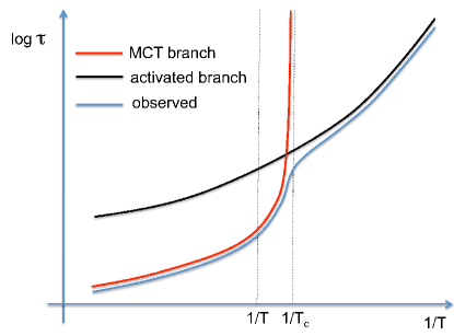
Figure 12: A schematic view of bulk relaxation. We hypothesise that there are two different channels of relaxation: i) the Mode Coupling Theory (MCT) channel, which is related to a relaxation which uses unstable stationary points (saddles) of the potential energy. The MCT dynamics has a relaxation time that diverges at $T_{c}$. ii) the activated barrier-crossing channel. The actual dynamics “chooses” the fastest of the two channels, so that the observed relaxation time is the lowest of the two. Below $T_{c}$, there is a dynamical crossover between the MCT branch to the activated branch. The crossover is exaggerated here to illustrate the point, the actual behavior is much smoother in the $T\sim T_{c}$ region.

We make the hypothesis that the real (observed) relaxation time of the system is the lowest of the two relaxation times, because the dynamics always follows the fastest relaxation channel. We can then get an impression of what happens in Fig. 12. The observed time follows the MCT branch up to close to $T_{c}$, where it crosses over to the activated branch, thus avoiding the MCT divergence. This hybridization between MCT and activated branches is (very roughly speaking) the origin of the dynamical crossover near $T_{c}$ Biroli and Bouchaud (2009).

Consider now what happens to this scenario when we use a swap dynamics. In general the activated relaxation time can be written as,

$$\tau_{\mathrm{ACT}}=\tau_{0}\exp(\xi_{s}^{\psi}/T),$$ (16)

where $\xi_{s}$ is the static correlation length. The effect of swap dynamics is essentially to decrease significantly the prefactor $\tau_{0}$ in equation (16) Fernández et al. (2006),

$$\tau_{\mathrm{ACT}}^{\mathrm{swap}}=\tau_{0}^{\mathrm{swap}}\exp(\xi_{s}^{\psi}/T),\qquad\mbox{with }\tau_{0}^{\mathrm{swap}}\ll\tau_{0}.$$ (17)

This amounts to a downward shift of the activated branch (Fig. 13). Due to this, the hybridization between the two branches disappears, and the observed relaxation time does not display any significant crossover close to $T_{c}$. We also see that if we fix a temperature $T\gtrsim T_{c}$, in the nonswap case the bulk time is dominated by the MCT channel, whereas in the swap case it is dominated by the activated channel (also see Fig. 1 of ref. Fernández et al. (2006), which shows how the MCT plateau seen in time correlation functions is lost with swap dynamics).

VIII.1.2 The cavity

Let us now turn to the cavity, bearing in mind that the large $R$ value of $\tau(R)$ is nothing else than the bulk time, whose behavior we have just examined. It has been suggested that the MCT cavity relaxation time, as a function of $R$, should have a divergence at $R\sim\xi_{d}$, where $\xi_{d}$ is the dynamic correlation length Franz and Montanari (2007). A possible interpretation of this fact is that in a smaller cavity the frozen boundary conditions stabilize unstable saddles, thus increasing the MCT relaxation time. Below $\xi_{d}$ the cavity runs out of saddles and nonactivated relaxation becomes impossible. On the other hand, the activated relaxation time obeys the scenario described by eqs. (7) and (8): it increases with $R$, saturating at the static correlation length, $\xi_{s}$.

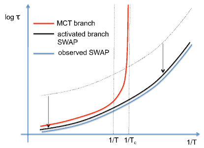
Figure 13: When we use a swap dynamics we are significantly lowering the prefactor of activated barrier crossing, hence shifting the activated branch downwards. As a result, there is no significant hybridization between the two branches and the resulting (observed) swap relaxation time does not detect any particular crossover close to $T_{c}$.

As for the bulk, we can speculate that the observed relaxation time in the cavity will be the smallest of the two times. Let us fix a temperature slightly above $T_{c}$, so that the nonswap bulk relaxation is dominated by the MCT channel (Fig. 12). In Fig. 14 we get a picture of what happens. Let us start from large values of $R$: the relaxation time follows the MCT branch, therefore giving an increase of $\tau(R)$ for decreasing $R$. But at some point the MCT branch crosses the activated one (and it eventually diverges at $\xi_{d}$), so beyond this point the dynamics sticks to the activated channel, giving rise to a maximum of $\tau(R)$. Hence, for small values of $R$ we recover a regime where $\tau(R)$ decreases for decreasing $R$.

The large $R$ regime of this nonmonotonic curve was also discussed in Biroli and Bouchaud (2009), where it was noted that above $T_{c}$ $\tau(R)$ should approach its bulk value from above. This behavior, namely a relaxation time that increases from its bulk value when decreasing $R$, is indeed what we find with nonswap dynamics, Fig. 10. However, in the nonswap case the increase of the relaxation time is so sharp that we struggle to follow this curve down to medium-small $R$, so we cannot access the overshooting.

What happens when we use swap dynamics? As in the bulk, by using swap we are decreasing the prefactor of activation, thus shifting the whole activated branch downwards. From Fig. 15 we see that this shift has the effect to weaken, or even wash out entirely, the nonmonotonic behavior of $\tau(R)$. Something similar happens by lowering the temperature (getting closer to $T_{c}$), because in that way we are narrowing the difference between the MCT and the activated branch (Fig. 12). In the cavity, this amounts to closing the gap between the two branches at large $R$. Hence, we expect that lowering $T$ too has the effect to iron out the maximum of $\tau(R)$, eventually making it disappear . Summarizing, we expect swap dynamics to display little sign of a nonmonotonic cavity relaxation time $\tau(R)$, and to become completely monotonic at low $T$. In Fig. 16 we show a close-up of the cavity relaxation time with swap dynamics at two different temperatures: there is an overshooting of $\tau(R)$ at intermediate temperature, but it completely disappears a the lowest $T$. This expectation is therefore supported by the data.

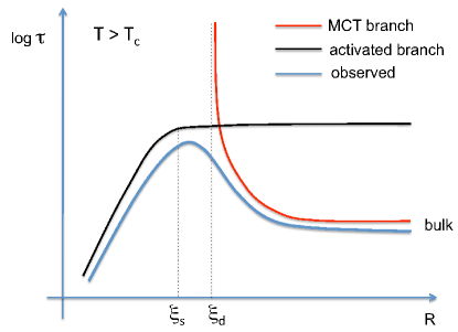
Figure 14: In the cavity, for $T\gtrsim T_{c}$ the hybridization between MCT and activated branch may give rise to a nonmonotonic $\tau(R)$. Starting from large cavities, the relaxation time follows the MCT branch, which has a divergence at the dynamical correlation length, $\xi_{d}$. In the proximity of such divergence the observed $\tau(R)$ crosses over to the activated branch, thus decreasing with decreasing $R$.

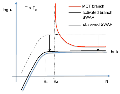
Figure 15: When we use swap dynamics in the cavity we shift the whole activated branch downwards, hence lowering the degree of hybridization of the two branches. In this way, the overshooting of relaxation time may be completely washed out, and $\tau(R)$ have a purely monotonously increasing behavior.

According to this scenario (admittedly based on little evidence), in the nonswap case one should see an increase of $\tau(R)$ over its bulk value when decreasing the cavity size from large $R$ (saturation from above), whereas in the swap case (and at low $T$) the cavity relaxation time should decrease below its bulk value when decreasing the radius (saturation from below). This prediction seems to be in qualitative agreement with our numerical findings. However, there is a severe problem with this interpretation, namely the fact that nonswap dynamics at very small $R$ is stuck. Even assuming that the great increase of the cavity relaxation time that we observe in going from large $R$ down to medium $R$ (Fig. 9) has to be identified with the large $R$ regime of a nonmonotonic $\tau(R)$ (Fig. 14), the question remains: why we do not see any hint of the low $R$ regime of Fig. 14, where the cavity relaxation time gets smaller for small radii? It is well possible, in this scenario, that for intermediate $R$ the relaxation time is significantly larger than the bulk limit. However, for very small $R$ the relaxation time should drop again. Yet, we do not see this. In fact, very small cavities are completely stuck, as shown in Fig. 11. This phenomenon is in open disagreement with our theoretical expectation. We must address this inconsistency.

Figure 16: Cavity relaxation time with swap dynamics. This is a zoom-in of Fig. 5, made to emphasize the nonmonotonic behavior of $\tau(R)$. At the highest temperature (open squares, $T=0.350$) there is an overshooting of $\tau(R)$, caused by the hybridization between the MCT and activated branches. At the lowest temperature (filled circles, $T=0.202$) the overshooting disappears due to the decreased gap between the MCT and the activated branch. The relaxation times are normalized by their bulk value.

VIII.2 The role of boundary rearrangements

The fact that swap dynamics thermalizes a small cavity quite rapidly while nonswap dynamics remains stuck, is weird; it indicates that swapping different particles in a small volume becomes prohibitive for standard dynamics. Of course, the exchange of two particles for the standard dynamics is the result of many moves, and it is for sure a more complicated process. Yet swapping two nearby particles is definitely not a terribly collective rearrangement and it should not implicate a very large activation barrier. If it does, it means that this barrier has been made dramatically large by the amorphous boundary conditions. Why is that?

A possible explanation is that by freezing the external configuration we are preventing the surrounding system to elastically accommodate for the small rearrangements within the cavity. Although exchanging two particles is not a collective rearrangement, i.e. one in which many particles move a lot, to happen it still needs that many particles make very small movements. This phenomenon was studied in ref. Grigera et al. (2002), where the distribution of particle displacements in moving from a local energy minimum to nearby one connected by a saddle of order $1$ was calculated. It was found that this process corresponds to few particles (order 2–3) moving an amount comparable to the interparticle distance and many particles moving very little, just to make space to the rearranging ones. Elasticity is also a central ingredient in the local elastic expansion model (also called “shoving model”) of viscous relaxation Dyre et al. (1996). More in general, one might argue that the whole short-time dynamics (not only elastic modes) plays a relevant role.

By freezing all the particles in the configuration external to the cavity we are inhibiting this contribution, perhaps making unnaturally large an otherwise modest barrier. Swap dynamics, on the other hand, needs not to pass through the top of a barrier to exchange two particles, and therefore is less affected by the suppression of the high-frequency response, and by the subsequent barrier’s increase. This may be the origin of the very different qualitative behavior of swap vs. nonswap dynamics observed at low $R$.

To check this last hypothesis, we suggest in the next Section a general approach to restore the short-time dynamics which is not limited to the elastic case, suggested by an alternative description of the problem in the RFOT spirit.

IX Frozen configuration vs. frozen state

An alternative description of the over-constraining due to the boundary can be given in terms of configurations vs. states. The original aim of the amorphous boundary conditions Bouchaud and Biroli (2004) was to keep the system surrounding the cavity within one fixed state (say $\alpha$), one of the exponentially many metastable states the supercooled liquid phase is composed of Kirkpatrick et al. (1989). According to this spirit, the external particles should be allowed to move enough to visit the many configurations belonging to state $\alpha$, but not enough to reach configurations that do not belong to $\alpha$. By choosing and fixing just one configuration within state $\alpha$, however, we are over-constraining the amorphous boundary, and this may have some side-effects on the dynamics of small rearrangements in the cavity when a standard dynamics is used.

In view of this, it seems reasonable to try to relax the constraint on the outer particles by changing the current frozen configuration (FC) setup, in favour of a frozen state (FS) one. This means that instead of completely freezing the particles outside the sphere, we let them relax subject to the condition that the overlap $q_{\mathrm{ext}}$ between the initial external configuration and the one at time $t$ remains at some value $\hat{q}_{\mathrm{ext}}$. The FC setup would be recovered taking simultaneously the limits $q_{\mathrm{ext}}\to 1$ and $\ell\to 0$. In this way, the external configuration is not allowed to move at all, so this amounts to a complete freezing.

Of course, the choice of $\hat{q}_{\mathrm{ext}}$ is critical: with too large a value we go back to the frozen configuration case, while too small a value destroys any point-to-set correlation in the cavity. In fact, in the limit $\hat{q}_{\mathrm{e}xt}=0$ the cavity must be ergodic and the overlap must relax to zero for any value of $R$. A sensible physical choice is,

$$\hat{q}_{\mathrm{ext}}=q_{\mathrm{EA}},$$ (18)

where $q_{\mathrm{E}A}$ is the self-overlap of a metastable state. In this way we ensure that the external system does not make any major structural rearrangement, and yet allows for minor movements of the particles, which can have an important elastic effect. To chose the correct value of $q_{\mathrm{EA}}$ we use the thermodynamic potential $V(q)$ recently discussed in Cammarota et al. (2010), whose secondary minimum indicates the value of the self-overlap $q_{\mathrm{E}A}$. At the temperature $T=0.246$, where we will run the FS simulations, a reasonable choice is (see Fig. 5 of ref. Cammarota et al. (2010)),

$$q_{\mathrm{E}A}=0.4.$$ (19)

Of course, the final test for this choice is that the point-to-set correlation must not be lost: having switched from a FC to a FS setup will certainly imply that the infinite time limit of the overlap, $q(R)$, will be smaller at all values of $R$. What we need is $q(R)\neq 0$ at for some range $[0:R]$, in order to have a physically significant point-to-set correlation function.

X Cavity dynamics with frozen state boundary conditions

X.1 FS simulations: technical details

First, we need to make a technical, but relevant, remark. In this work, as well as in previous works Cavagna et al. (2007); Biroli et al. (2008), the overlap is defined in such a way that it does not detect the exchange of particles of different size. The same definition has been adopted by other groups Berthier and Kob (2011); Berthier et al. (2011). However, we cannot use this definition for imposing the constraint on the external particles: an exchange of two different particles, perhaps quite far from each other, must not be allowed. Hence, the constraint must be imposed on an overlap that is sensitive to the exchange of particles of different kind (whereas we still do not distinguish the exchange of identical particles). Let us call this the binary overlap, defined as

$$q_{\mathrm{bin}}(t)\equiv\frac{1}{\ell^{3}\,N_{i}}\sum_{i\in v}\left[n_{i}^{A}(0)n_{i}^{A}(t)+n_{i}^{B}(0)n_{i}^{B}(t)\right],$$ (20)

where $n_{i}^{X}(t)$ is the number of particles of kind $X$ in box $i$. This is also the definition used in Cammarota et al. (2010) to compute the thermodynamic potential $V(q)$. In what follows we thus use $q_{\mathrm{bin}}$ to put the constraint on the outside particles. On the other hand, in order to compare with the previous results, we continue using the standard overlap within the cavity.

Conceptually, FS simulations are straightforward: we simply reject all moves on the external particles that violate constraint (18). In practice, FS simulations are much more demanding than FC ones, because now we have to update all particles in the system, not simply those within the cavity. For this reason we restricted our investigation of the frozen state setup to just 3 cavity sizes, $M=20,50,100$ particles, corresponding to $R=1.68,2.27,2.88$, and to just one temperature, $T=0.246$.

X.2 FS simulation results

The first thing we have to check is what happens to the point-to-set correlation function, i.e. to the asymptotic value of the overlap, $q(R)$, in the FS setup at this value of the temperature. To do this we run a swap BIC test in the FS setup, to be sure to get the thermalized asymptotic overlap. We report these values in Table I, where we also report the corresponding values for the standard FC setup. Recall that the effective zero of the overlap, i.e. the value it has for two uncorrelated configurations, is $q_{0}=0.062876$.

Table 1: Point-to-set correlation function $q(R)$: FS vs. FC

$M$	$R$	$q^{\mathrm{FS}}(R)$	$q^{\mathrm{FC}}(R)$
20	1.68	0.222 $\pm$ 0.004	0.578 $\pm$ 0.001
50	2.27	0.142 $\pm$ 0.003	0.479 $\pm$ 0.001
100	2.88	0.095 $\pm$ 0.002	0.314 $\pm$ 0.002

As expected, there is a significant decrease of $q(R)$ in the FS case, due to the fact that particles in the external configuration are now partly free to move, hence lowering the constraint on the inner particles. However, in the FS case $q(R)$ is still nonzero, so that the PTS correlation function is nontrivial. We stress that the values in Table I have been obtained from a swap BIC test: the lower branch of the BIC test grows with time up to its asymptotic limit. We are therefore quite sure that the FS values of $q(R)$ that we report are nonzero.

Next, we turn to the time series of the overlap $q(t)$ in the FS setup, compared to the FC setup. We stress, once again, that we are using standard nonswap Montecarlo dynamics, both for FC and FS. The data are reported in Fig. 17 for three different values of $R$. In order to make the FS/FC comparison easier, we plot the connected overlap, i.e. the overlap subtracted by the (swap) equilibrium value, $q(R)$. The connected overlap must go to zero for infinite time.

At these values of $T$ and $R$, the FC time series (dashed lines) are completely stuck at an off-equilibrium value, so much as to make it impossible to even estimated the relaxation time. We already observed this phenomenon in Fig. 11. On the other hand, the FS time series (full lines) are quite different: the overlap does not remain stuck at any specific level; in fact, it seems to be decaying steadily towards zero. Unfortunately $2$ million Monte Carlo steps (our largest time) are not enough to directly observe the point where the connected overlap goes to zero. However, a reasonable extrapolation suggests that for all three values of $R$ the relaxation time is somewhere between $10^{6}$ and $10^{7}$ Monte Carlo steps.

Figure 17: Frozen configuration (FC) vs. frozen state (FS) setup, standard nonswap dynamics. We plot the connected overlap, obtained by subtracting its equilibrium infinite time limit $q(R)$ (obtained with a swap BIC test). The asymptotic equilibrium value of the connected overlap is zero. The three values of $R$ investigated here are small, so that the FC dynamics (dashed line) is completely stuck at an out of equilibrium level. On the contrary, the FS dynamics (full line) is not stuck and, even though longer runs would be needed, it is approaching equilibrium. $T=0.246$.

Figure 18: Frozen configuration (FC) vs. frozen state (FS) setup, standard nonswap dynamics. We plot the standard overlap (lines) and the binary overlap (symbols). These two overlaps are the same as long has no particles of different size have been swapped. On the other hand, when the (nonswap) dynamics starts swapping particles, the binary overlap gets smaller than the standard one. This never happens in the FC setup (upper panel), whereas it happens for sufficiently long times in the FS setup (lower panel). This fact explains why the FC dynamics is stuck, while the FS one is not. $R=2.88$, $T=0.246$.

We conclude that the cavity dynamics with frozen state boundary condition no longer remains stuck at an off-equilibrium level. This result goes in the direction we expected: allowing the in-state vibrations of the external configuration unleashes some minor, but necessary, relaxation modes that are otherwise frozen in the FC setup. In particular, what happens is that in the FS case even a nonswap dynamics is able (after a while) to exchange different particles, while in the FC case this never happens. This phenomenon is shown in Fig. 18. We report in this figure the standard cavity overlap, $q(t)$, and the binary cavity overlap, $q_{\mathrm{bin}}(t)$, which is sensitive to the exchange of different particles. What we see is that in the FC setup (upper panel) the two overlaps coincide up to the longest time, meaning that particles exchanges never happen. On the other hand, in the FS setup (lower panel) there is a decoupling between the two overlaps at about $5\times 10^{5}$ Monte Carlo steps (this decoupling is also found in FC swap dynamics —not shown— where it is naturally expected since the swap moves consist precisely in the exchange of two particles of different kind). Hence, even the nonswap dynamics is able to swap particles in the long run, and therefore to relax the cavity, provided that we confine the external system within a state, rather than a configuration.

The last, and most important, open issue is the behavior of the relaxation time as a function of $R$. We recall here the situation schematically summarized in Fig. 14: the relaxation time for medium $R$ can be significantly larger that the bulk time, due to the hybridization of the MCT and activated branches. However, for small enough $R$ one should go back to a regime where $\tau$ decreases for decreasing $R$. This overshooting scenario is what happens with a local swap dynamics, Fig. 16, and our expectation was that it should also happen with a normal nonswap dynamics, provided that we use an FS setup. Is this scenario confirmed or disproved by the data in Fig. 17?

Longer simulations (at least one order of magnitude longer) and several more values of $R$ and $T$ would be required to clear up unambiguously this matter. However, an unscrupulous extrapolation of the data in Fig. 17 suggests that the intermediate sized cavity, $R=2.27$, has the largest relaxation time, definitely closer to the right side of the $[10^{6}:10^{7}]$ window, whereas the smallest and largest cavities, $R=1.68$ and $R=2.88$, both seem to have a smaller relaxation time, closer to the $10^{6}$ side. In other words, the smallest cavity seems not to be the slowest one. If this were true, it would mean that we are exactly around the maximum of $\tau(R)$ in Fig. 14 and that we are starting to see a hint of the expected decrease of $\tau$ with decreasing $R$. Needless to say, we cannot push this interpretation of the data too far. Let us be content to say that current simulations with frozen state boundary conditions and nonswap dynamics do not rule out the existence of a low $R$ regime where smaller cavities have smaller relaxation times.

Further work to clear up this issue is currently in progress. Unfortunately there is no easy way to settle this. We cannot use smaller cavities, because $M=20$ particles is already about the smallest reasonable size in three dimensions. The only thing to do is to push the simulations at longer times, which is computationally very costly.

XI Some experimental evidence

At the experimental level, there has been considerable interest in studying liquids in confinement conditions, in particular since nanoporous materials with well-defined pore radius have been available (see Liu et al. (1989); Zhang et al. (1992); Arndt et al. (1997) and references therein) and more recently materials such as carbon nanotubes Rasaiah et al. (2008).

For liquids confined in nanopores the experimental glass transition temperature (as measured with differential scanning calorimetry) is reduced as the pore becomes smaller Zhang et al. (1992), i.e. confined systems are faster than the bulk. However, the situation is rather more complicated, as relaxation experiments Liu et al. (1989); Arndt et al. (1997) point to the existence of at least two regions in space, with different dynamics: a slow layer of molecules directly in contact with the pore walls and a fast region inside the cavity and far from the walls.

A particularly interesting case is reported in ref. Arndt et al. (1997): the relaxation time of salol confined in nanoporous silica glass was found with dielectric relaxation measurements (unable to distinguish the interfacial and central regions of the pore) to be larger for increasing confinement. However, after coating the pore walls with a hydrophobic lubricant (thus reducing the H bonds between salol and the pore surface) it was found that smaller cavities are faster. In particular, they are significantly faster than the bulk. Hence, in this experimental case, once the interactions that slow down the interfacial layer were supressed, the relaxation time as a function of the radius has a qualitative behavior similar to Fig. 3. The authors of ref. Arndt et al. (1997) used this to determine a cooperativity length scale.

There are intriguing similarities, as well as obvious differences, with our case. In both cases the original interaction with the cavity interface was too stiff, suppressing some relaxation channels that are not cooperative, and yet necessary to equilibrate the cavity. The strategy in Arndt et al. (1997) was to lubricate the inside of the cavity, thus hindering the H bonds responsible for the artificial slowing down; our strategy was the make the surrounding system softer. In the experimental case the effect was clear: lubricated cavities are faster than unlubricated ones; smaller cavities are faster than larger cavities. In our case, we also obtain that FS cavities are faster than FC cavities; whether or not smaller cavities are faster than larger ones is unclear, but the data do not rule this out.

The differences are also relevant. In the experimental case the confined (free) system is liquid salol, and the pore is glass. Hence, even though one may say that there are amorphous boundary conditions, these are certainly not drawn from the Gibbs-Boltzmann equilibrium distribution of an external salol system. Moreover, the reasons for the original ‘stiffness’ are also different. In the experimental case it is the formation of H bonds between internal salol and the surface of the pore. In our case, the nature of the bonds between particles within the cavity and across the interface is exactly the same; however, the complete freezing of the cavity suppresses the swap, uncooperative, rearrangements useful to reach equilibrium. Accordingly, the solutions adopted are also different.

We cannot not say whether or not the similarities overcome the differences, so to make this experimental case significant to our context. We limit ourselves to register the fact that the problem of an artificial slowing down in confining geometries has already occurred in experiments and that, when solved, the cavity dynamics can change very dramatically.

XII Conclusions

We have studied the dynamics of a confined cavity, using different Montecarlo algorithms and different amorphous boundary conditions. Our bare findings are:

1. FC—swap—low $T$: the cavity relaxation time $\tau$ is larger the larger $R$ and it saturates at $R\sim\xi_{s}$, where $\xi_{s}$ is the point-to-set correlation length.

2. FC—swap: in the region $R\sim\xi_{s}$ a colder cavity relaxes faster than a hotter cavity.

3. FC—swap: at higher $T$ the relaxation time $\tau(R)$ displays an overshooting that disappears on lowering $T$.

4. FC—nonswap: $\tau$ is larger the smaller $R$.

5. FC—nonswap: small cavities ($R<4$) are completely stuck at an off-equilibrium level.

6. FS nonswap dynamics is significantly faster than FC nonswap dynamics; with FS small cavities are no longer stuck.

7. The FS point-to-set correlation function $q(R)$ is nonzero in the region of interest of $T$ and $R$.

8. FS—nonswap: data are compatible with a nonmonotonic $\tau(R)$; data do not rule out the possibility that in small cavities $\tau$ is smaller the smaller $R$.

We have proposed a theoretical scenario whose aim is to organize all these results into one coherent picture. Our scenario rests on two main ideas. First, depending on the values of $R$ and $T$, and on the type of dynamics, there may be an hybridization between MCT and activated relaxation channels; this hybridization, when present, gives rise to a nonmonotonic cavity relaxation time $\tau(R)$. Second, the frozen configuration setup is unsuitable to run nonswap dynamics, and in general it is not very physical, as it may give rise to an artificial dynamical freezing. We have introduced a frozen state setup, based on the idea that the amorphous boundary condition must select a certain state, not simply a certain configuration. If we trust these two ideas, then we can find an interpretation for the very diverse results we find.

Result 1 supports the concept that $\xi_{s}$ is the relevant scale of cooperativity in the system. According to the RFOT theory with fluctuating surface tension, the activated relaxation time is equal to the in-state relaxation time for $R\ll\xi_{s}$, it grows when $R$ gets across the support of the probability distribution of the rearranging sizes $P(R,\xi_{s})$, and it finally saturates to its bulk value for $R\gg\xi_{s}$. Hence, when the cavity is larger than the scale of cooperativity relaxation factorizes, whereas when the cavity is smaller than $\xi_{s}$ the whole cavity must rearrange collectively. This RFOT interpretation is supported by result 2: an inversion of the relaxation time (cooler is faster) happens because a colder cavity may still be confined within just one state, thus showing only the short, in-state relaxation time, while (at the same value of $R$) a hotter cavity may be already unlocked, thus sporting the full bulk relaxation time.

The maximum displayed by the local swap $\tau(R)$ (result 3) is one piece of evidence in support of the (rather speculative) scenario described in Section VIII: the hybridization between nonactivated MCT channels and activated channels gives rise in the bulk to the crossover between MCT and activation close to $T_{c}$, while in the cavity it gives rise to a nonmonotonic $\tau(R)$. This hybridization implies that for large $R$ the cavity relaxation time follows the MCT branch, so that $\tau$ is larger the smaller $R$, which is in agreement with the nonswap dynamics result 4. On the other hand, switching to swap dynamics has a twofold effect: in the bulk, it eliminates the $T_{c}$ crossover; in the cavity, it flattens the maximum of $\tau(R)$.

We have speculated that the complete freezing out of small cavities with nonswap dynamics (result 5) is not quite physical, and we have suggested that it could be the effect of an artificial suppression of some elastic (noncooperative) relaxation modes due to the frozen configuration setup. We have proposed a practical way to implement amorphous boundary conditions with a frozen state and we have found that this setup speeds up significantly the nonswap dynamics, unlocking the small cavities (result 6). We have also checked that the point-to set correlation remains nonzero, despite a significant reduction due to the smaller degree of confinement by the external state (result 7).

Finally, we tried to understand what was the behavior of $\tau$ as a function of $R$ in the frozen state case. This is quite crucial: if we cannot find any regime of $R$ and $T$ where the nonswap $\tau$ is smaller for smaller $R$, then we have a problem. Our entire construction relies on the idea that for small enough $R$ the MCT branch must be gone, so that all that remains is the activated branch, and this must be faster the smaller the cavity. Our time series (Fig. 17) are too short to settle this matter. But we can at least say that the data do not rule out this possibility (result 8). With a little more optimism, we can even conclude that the smallest cavity is not the slowest one, which is all we need to support our theoretical scenario.

The whole scenario still admits considerable improvements in clarity. As we have said, longer simulation with nonswap dynamics in the FS setup are needed to study carefully $\tau(R)$, and this should be done at several values of $R$ and of $T$. At the same time, FS swap simulations should be run in order to reconstruct the entire point-to-set correlation function, $q(R)$, to check whether or not it retains its essential properties. Is it still a nonexponential function at lower temperature? How does the FS correlation length $\xi_{s}$ compare to its FC counterpart? Work in this direction is in progress.