The generalized second law in universes with quantum corrected entropy relations

Abstract

We apply the generalized second law of thermodynamics to discriminate among quantum corrections (whether logarithmic or power-law) to the entropy of the apparent horizon in spatially Friedmann-Robertson-Walker universes. We use the corresponding modified Friedmann equations along with either Clausius relation or the principle of equipartition of the energy to set limits on the value of a characteristic parameter entering the said corrections.

I Introduction

As is well known, event horizons, whether black holes’ or cosmologicals, mimic black bodies and possess a nonvanishing temperature and entropy, the latter obeying the Bekenstein-Hawking formula, bekenstein73 ; davies75 ; gibbons77

$$S_{BH}=k_{B}\frac{A}{4l^{2}_{pl}}\,.$$ (1)

This expression, in which $k_{B}$ stands for the Boltzmann constant, $A$ the area of the horizon, and $l_{pl}=\sqrt{G\hbar/c^{3}}$ the Planck’s length, points to a deep connection between gravitation, thermodynamics, and quantum mechanics, still far from being fully unveiled though progress in that direction are being made -see, e.g., wu08a ; wu08b and references therein. Recently it was demonstrated that cosmological apparent horizons are also endowed with thermodynamical properties, formally identical to those of event horizons cai09 .

The connection between gravity and thermodynamics was reinforced by Jacobson, who associated Einstein equations with Clausius’ relation jacobson95 , and later on by Padmanabhan who linked the macroscopic description of spacetime, given by Einstein equations, to microscopic degrees of freedom, $N$, through the principle of equipartition of energy, i.e.,

$$E=\frac{1}{2}Nk_{B}T\,.$$ (2)

In particular, Padmanabhan, starting from the field equations arrived to the equipartition law padmanabhan10b and indicated how to obtain the field equations of any diffeormorphism invariant theory of gravity from an entropy extremising principle padmanabhan07 , the entropy of spacetime being proportional to $N$.

On the other hand, quantum corrections to the semi-classical entropy-law (1) have been introduced in recent years, namely, logarithmic and power-law corrections. Logarithmic corrections, arises from loop quantum gravity due to thermal equilibrium fluctuations and quantum fluctuations meissner04 ; ghosh04 ; chatterjee04 ,

$$S\propto\left[\frac{A}{4l^{2}_{pl}}+\alpha\ln{\frac{A}{4l^{2}_{pl}}}\right]\,.$$

On its part, power-law corrections appear in dealing with the entanglement of quantum fields in and out the horizon saurya08 ,

$$S\propto\frac{A}{4l^{2}_{pl}}\left[1-K_{\alpha}A^{1-\alpha/2}\right]\,.$$

In the last two expressions, $\alpha$ denotes a dimensionless parameter whose value (in both cases) is currently under debate.

For the connection between horizons and thermodynamics to hold, these quantum entropy corrections must translate into modifications of the field equations of gravity, see e.g. lidsey09 ; cai09 ; zhang10 . In any sensible cosmological context these modifications must fulfill the generalized second law (GSL) of thermodynamics. The latter asserts that the entropy of the horizon plus the entropy of its surroundings must not decrease in time. As demonstrated by Bekenstein, this law is satisfied by black holes in contact with their radiation bekenstein74 .

The aim of this paper is to see whether the modified Friedmann equations coming from logarithmic corrections and from power-law corrections, in conjunction with Clausisus relation or the equipartition principle, are compatible with the generalized second law. This will set constraints on the parameter $\alpha$ introduced above, whose value is theory dependent and rather uncertain. We hope this may be of help in discriminating among quantum corrections, via a purely classical analysis.

The plan of this work is as follows: Section II derives Friedmann equations from different entropy corrections, considering a Friedmann-Robertson-Walker (FRW) metric sourced by a perfect fluid. Section III considers the entropy rate enclosed by the apparent horizon and in which the fluid is in thermal equilibrium with it. Section IV e xtends the analysis by allowing the fluid to be phantom, for a period, or by allowing the production of particles. Finally, Section V summarizes and discusses our findings.

II Modified Friedmann equations

In this section we recall the derivation of the modified Friedmann equations in case of the classes of entropy corrections to the Bekenstein-Hawking entopy in eq.(1). As said above, this semiclassical relation gets modified when quantum corrections are taken into account.
Logarithmic corrections lead to the expansion meissner04 ; ghosh04 ; chatterjee04

$$S=k_{B}\,\left[\frac{A}{4l^{2}_{pl}}+\alpha\ln{\frac{A}{4l^{2}_{pl}}}\right],$$ (3)

while power-law corrections yield saurya08

$$S=k_{B}\,\frac{A}{4l^{2}_{pl}}\left[1-K_{\alpha}A^{1-\alpha/2}\right],$$ (4)

for the horizon entropy. In (4) $K_{\alpha}$ is a parameter that depends on the power $\alpha$ of the entropy correction.
We wish to examine thermodynamical behavior of the system consisting in the apparent horizon of a spatially flat FRW universe and the fluid within it.
The FRW metric can be written as

$$ds^{2}=h_{ab}dx^{a}dx^{b}+\tilde{r}^{2}d\Omega^{2},$$

where $\tilde{r}=a(t)r$ and $h_{ab}=\text{diag}(-1,a(t)^{2})$. The apparent horizon is defined by the condition $h^{ab}\partial_{a}\tilde{r}\partial_{b}\tilde{r}=0$ so that its radius turns out to be

$$\tilde{r}_{AH}=\frac{c}{H},$$ (5)

where $H=\dot{a}/a$ denotes the Hubble function. From expressions (3) and (4) different cosmological scenarios can be considered, depending on whether use is made of Clausius relation jacobson95

$$\delta Q=TdS\,,$$ (6)

or the principle of equipartition of the energy, $dE=k_{B}d(NT)/2$ padmanabhan10a . In either case, the left hand side represents the amount of energy that crosses the apparent horizon within a time interval $dt$ in which the apparent horizon evolves from $\tilde{r}_{AH}$ to $\tilde{r}_{AH}+d\tilde{r}_{AH}$

$$dE=A_{AH}T_{\mu\nu}k^{\mu}k^{\nu}dt\,.$$

Here $T_{\mu\nu}=(\rho+P/c^{2})u_{\mu}u_{\nu}+Pg_{\mu\nu}/c^{2}$ is the energy-momentum tensor of the perfect fluid, and $k^{a}$ is the approximate generator of the horizon, $k^{a}=(1,-Hr,0,0)$. It follows that

$$dE=4\pi\tilde{r}^{3}\left(\rho+\frac{P}{c^{2}}\right)\ H\ dt.$$ (7)

The change of the area of the apparent horizon, $dA_{AH}=8\pi\tilde{r}_{AH}d\tilde{r}_{AH}$, induces the entropy shift,

$$dS=\frac{\partial S}{\partial A}dA=-\frac{8\pi\tilde{r}_{AH}^{4}}{c^{2}}\frac{\partial S}{\partial A}H\dot{H}dt\,.$$ (8)

The number of degrees of freedom is assumed proportional to the entropy whereby it also changes, and the same holds true for the temperature of the system, that we take as the temperature of the horizon cai09

$$T_{H}=\frac{\hbar}{k_{B}}\frac{c}{2\pi\ \tilde{r}_{AH}}\,.$$ (9)

By using eq.(7) with either Clausius relation (6) or the equipartition principle (2), one gets the modified Friedmann equations,

$$H^{2}\left[1+g(\alpha,H)\right] = \frac{8\pi G}{3}\rho,$$ (10)

$$\dot{H}\left[1+f(\alpha,H)\right] = -4\pi G\left(\rho+\frac{P}{c^{2}}\right),$$ (11)

the explicit expressions of $f(\alpha,H)$ and $g(\alpha,H)$ depend on both the entropy corrections and the thermodynamical relation employed, as shown in Table 1. It should be noted that, eq.(10) can be recovered from eq.(11) and the evolution equation for the perfect fluid:

$$\dot{\rho}+3H\left(\rho+\frac{P}{c^{2}}\right)=0.$$ (12)

Table 1: Expressions for $f(\alpha,H)$ and $g(\alpha,H)$.

	Logarithmic correction
Equipartition	$f(\alpha,H)=\frac{l^{2}_{p}\alpha}{2\pi c^{2}}H^{2}\left\{1-\frac{1}{2}\ln{\left(\frac{\pi c^{2}}{l^{2}_{p}H^{2}}\right)}\right\}$
	$g(\alpha,H)=\frac{3l^{2}_{p}\alpha}{16\pi c^{2}}H^{2}\left\{1+\frac{2}{3}\ln{\left(\frac{\pi c^{2}}{l^{2}_{p}H^{2}}\right)}\right\}$
Clausius	$f(\alpha,H)=\frac{l^{2}_{p}\alpha}{2\pi c^{2}}H^{2}$
	$g(\alpha,H)=\frac{3l^{2}_{p}\alpha}{16\pi c^{2}}H^{2}$
	Power-law correction
Equipartition	$f(\alpha,H)=-\alpha\frac{3-\alpha}{4-\alpha}(Hr_{c})^{\alpha-2}$
	$g(\alpha,H)=-\frac{3-\alpha}{4-\alpha}(Hr_{c})^{\alpha-2}$
Clausius	$f(\alpha,H)=-\frac{\alpha}{2}(Hr_{c})^{\alpha-2}$
	$g(\alpha,H)=-(Hr_{c})^{\alpha-2}$

In the case of the logarithmic correction the two approaches differ by a logarithmic term that comes from the $NdT$ contribution. Moreover, contrary to Ref. zhang10 , we believe it should not be neglected because $\ln{(A_{AH}/l^{2}_{p})}$ is larger than zero when the area of the apparent horizon is of order of the Planck area.
On its part, power-law entropy correction gives the same correction to the Friedmann equations, the only difference lying in the value of the coefficients. The coefficient $r_{c}$, there, is related to the dimensionless parameter $\alpha$ by $K_{\alpha}=\alpha(4\pi)^{\alpha/2-1}/(4-\alpha)r_{c}^{2-\alpha}$.

As can be noted, the $\alpha$ parameter directly comes from quantum corrections to the entropy and it consequently affects cosmological scenarios. Its value depends on the details of the quantum calculations, and for the time being there is not agreement on it. The following analysis determines in which intervals this parameter results compatible with the GSL.

III The Generalized second law of Thermodynamics

Equipped with the entropy expressions (3) and (4), we set out to study whether the GSL is satisfied when the modified Friedmann equations (10) and (11) are employed.

Since the entropy depends on the area of the apparent horizon, $A_{AH}\propto H^{-2}$, it varies as

$$\dot{S}_{H}\propto F(H)\dot{H}.$$

Using eq.(11), it can be cast in terms of the Hubble parameter and the energy density and pressure of the fluid that fills the universe

$$\dot{S}_{H}=\mathcal{K}\frac{\mathcal{F}(H)}{H^{3}}\left(\rho+\frac{P}{c^{2}}\right),$$ (13)

where

$$\mathcal{K}=\frac{8\pi^{2}c^{5}k_{B}}{\hbar}$$

and $\mathcal{F}(H)$ depends on the entropy corrections and the thermodynamic relation used to derive Friedmann equations, namely

$$\mathcal{F}(H)=\frac{1+\frac{\alpha l_{p}^{2}H^{2}}{\pi c^{2}}}{1+f(\alpha,H^{2})},$$ (14)

for logarithmic entropy corrections, and

$$\mathcal{F}(H)=\frac{1+\alpha(r_{c}H)^{\alpha-2}/2}{1+f(\alpha,H)},$$ (15)

for power-law corrections.
For the sake of clarity in what follows we split the analysis for the two classes of entropy corrections, but in this section we will only consider perfect fluids assuming that the dominant energy condition (DEC) holds true (i.e., $\rho+P/c^{2}>0$) all along the expansion. Then, in view of eq.(13) the GSL is satisfied provided $\mathcal{F}(H)$ is non-negative which occurs only for some values of the parameter $\alpha$. In all the cases the results of general relativity davies87 are recovered, as it should, by setting $\alpha=0$.

III.1 Logarithmic entropy corrections

For convenience, we introduce the dimensionless variable $x=l^{2}_{p}/A_{AH}$ so that $x\simeq 1$ at the quantum regime and, provided $\dot{H}<0$, it decreases as time goes on. In terms of this new variable and using the equipartition theorem, eq.(2), we have that

$$\mathcal{F}(\alpha,x)=\frac{1+4\alpha x}{1+2\alpha x\left(1+\frac{1}{2}\ln{4x}\right)}.$$ (16)

We require $\mathcal{F}(\alpha,x)$ to be non-negative, if the GSL is to hold, as well as $\rho\geq 0$, not to deal with ghosts. From Friedmann’s equation (10) with $g(\alpha,H)$ given for the logarithmic correction of entropy, it translates into the condition

$$\frac{\rho}{H^{2}}\propto 1+g(\alpha,x)=1+\frac{3}{4}\alpha x\left(1+\frac{2}{3}\ln{4x}\right)\geq 0\,.$$ (17)

Fig.1 depicts the regions in the plane $(x,\alpha)$ where $\mathcal{F}>0$ is fulfilled and those in which $\mathcal{F}<0$. We believe that the allowed values for $\alpha$ are just those such that the GSL holds throughout the expansion of the Universe. The upper bound on $\alpha$ is given by the local minimum of the dashed curve, that is $\alpha=4e^{3}$, and the lower bound by the intersection of the dotted curve with the line $x=1$ (i.e., when horizon area equals Planck’s area), that is $\alpha=-1/4$ (not shown).

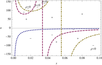
Figure 1: Plot of the sign of $\mathcal{F}$ depending on $\alpha$ along the Universe expansion, in the case of the logarithmic correction and the equipartition principle. Here, $x=l^{2}_{p}/A_{AH}$. The plot focuses on the range $0<x<0.1$ but in the remaining region the curves behave monotonically. Bear in mind that the smaller $x$, the older the universe is.

Positive values of $\alpha$ seem to be largely favored, which is also consistent with some quantum calculations of the entropy corrections hod04 .
By using Clausius relation (6), instead, and adopting the above defined variable $x$ we get

$$\mathcal{F}(x,\alpha) = \frac{1+4\alpha x}{1+2\alpha x},$$ (18)

$$\frac{\rho}{H^{2}} \propto 1+g(\alpha,x)=1+\alpha x.$$ (19)

As seen in Fig.2, the GSL is satisfied, $(\mathcal{F}(\alpha,x)\geq 0)$, for $\alpha>-1/(4x)$.

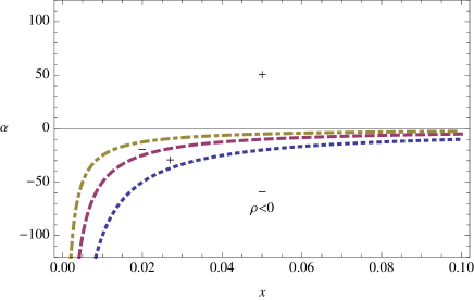
Figure 2: Same as Fig. 1 but with the equipartition principle replaced by Clausisus relation

.

III.2 Power-law entropy correction

Before applying the GSL let us look at the Friedmann equations for power-law entropy correction. Inspection of eq.(4) shows that the values of $\alpha=0$ and $\alpha=2$ are special, in the sense that for $\alpha=0$ there are no entropy corrections and the equations reduce to the corresponding general relativity expressions with a cosmological constant. Likewise $\alpha=2$ represents just a renormalisation of Newton constant, $G$. Bearing this in mind, we start the analysis by introducing the dimensionless variable $x=(r_{c}H)^{-1}$, and identifying the crossover scale $r_{c}$ with $H_{0}^{-1}$, as in dvali03 . Thus $x$ tends to zero in the far past and its today value is $x_{0}=1$ (provided, again, that $\dot{H}<0$).
By virtue of Clausius’ relation (6), the positive energy condition

$$1+g(\alpha,x)=1-x^{2-\alpha}\geq 0$$

implies

$$\alpha\leq 2.$$

Likewise, the function $\mathcal{F}$ in eq.(13) adopts the form

$$\mathcal{F}=\frac{1+\alpha x^{2-\alpha}/2}{1-\alpha x^{2-\alpha}/2},$$ (20)

and it is non-negative in the ranges

$$\left\{\begin{array}[]{ccc}\alpha<-2&\text{and}&0<x<\left(-\frac{\alpha}{2}\right)^{(2-\alpha)}\,,\\ -2\leq\alpha<2&\text{and}&0<x<1\,,\\ \end{array}\right.$$

as seen in Fig.3. The latter shows that the GSL remains valid throughout the expansion so long as $-2\leq\alpha<2$.

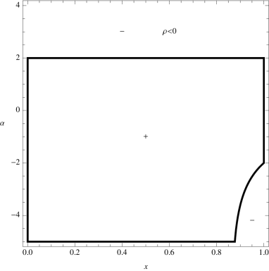
Figure 3: Sign of $\mathcal{F}$ depending on $\alpha$ along the Universe expansion in the case of power-law correction and Clausius relation. Here $x=H_{0}/H$.

.

When use is made of the equipartition relation one is led to the same functional modification of the Friedmann equations, $\propto H^{\alpha}$, but with different coefficients, which depend on $\alpha$. In this case, $\rho\geq 0$ implies

$$1+g(\alpha,x)=1-\frac{3-\alpha}{4-\alpha}x^{2-\alpha}\geq 0$$

and

$$\mathcal{F}=\frac{1+\alpha x^{2-\alpha}/2}{1-\frac{3-\alpha}{4-\alpha}\alpha x^{2-\alpha}}.$$ (21)

Now, $\mathcal{F}$ is non-negative in the following ranges

$$\left\{\begin{array}[]{ccc}\alpha<-2&\text{and}&0<x<\left(-\frac{\alpha}{2}\right)^{2-\alpha}\,,\\ -2\leq\alpha<2&\text{and}&0<x<1,\\ 2<\alpha<3&\text{and}&\left(\frac{\alpha(\alpha-3)}{\alpha-4}\right)^{2-\alpha}<x<1\,,\\ 3\leq\alpha<4&\text{and}&0<x<1\,.\\ \end{array}\right.$$

As can be easily learnt from Fig.4, this approach allows a wider range for the parameter $\alpha$ which can now lie in the range $3\leq\alpha<4$, as well.

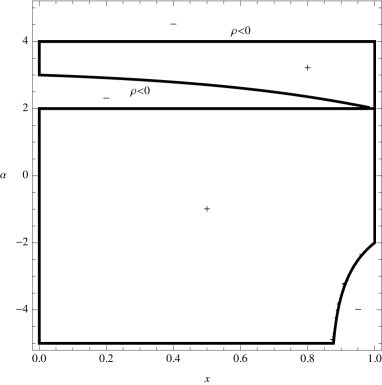
Figure 4: Same as Fig. 3 but with Clausius relation replaced by the equipartition principle.

IV GSL with phantom fluid or particle production

This section investigates whether by relaxing the dominant energy condition (DEC) or by allowing particle production, the range of values of $\alpha$ compatible with the GSL gets wider. The above analysis shows that this may be the case but there are regions where the GSL is still violated so long as ghost fields are excluded. In Figs. 1–4 these regions are explicitly marked.

IV.1 Phantom fluid

We begin with the logarithmic corrections to the horizon entropy. First we note that an equivalent rewriting of the entropy rate in eq.(13), for both eq.(16) and eq.(18), is

$$\dot{S}\propto(1+4\alpha x)\frac{\dot{H}}{H^{3}}.$$

Then, for non-superaccelerated expansion $(\dot{H}<0)$, the GSL will be fulfilled if $1+4\alpha x<0$. This means that we the line $\alpha=-1/4$ should not be crossed if a meaningful description of the expansion is required.
Nevertheless, we can focus on the positive range of the $\alpha$ parameter in case of equipartition of energy that, as inspection of Fig.1 reveals, can be enlarged from the minimum of the dashed curve, $\alpha=-(2x+x\ln{4x})^{-1}$, to the minimum of the dot-dashed curve, $\alpha=(3x+2x\ln{4x})^{-1}$, by allowing the fluid to be phantom during the evolution. These positive values of $\alpha$ may be seem too big, but they are not inconsistent with quantum calculations hod04 .
Let us note that, at present, $x_{0}=l^{2}_{p}H^{2}_{0}/4\pi c^{2}\sim 10^{-98}$. This means that the phantom phase lies far in the past. Could it give rise to a "reasonable" inflation? The first thing to check is whether there are accelerated phases in this modified theory of gravity (because of quantum corrections proportional to $\alpha$). Introducing the parameter $\gamma$ appearing in the equation of state, $p=(\gamma-1)\rho$, in the phantom region, when $\gamma<0$ and $\mathcal{F}<0$, positive values of $\alpha$ are compatible with acceleration $\ddot{a}>0$ provided that the inequality

$$\gamma>\frac{2(1+f(\alpha,H))}{3(1+g(\alpha,H))},$$

is fulfilled. Then, an inflationary period can be obtained for $4e^{3}<\alpha<8e^{5/2}$; the latter bound corresponds to the minimum of the dot-dashed curve in Fig.1.
For this early inflation to be successful in solving the problems of the standard big-bang model it must yield a sufficient number of e-folds, $N\sim 60$. Bearing in mind eqs.(10) and (11) we get

$$N=\int_{t_{i}}^{t_{f}}Hdt=-\frac{1}{3}\int_{x_{i}}^{x_{f}}\frac{1}{\gamma}\frac{1+f(\alpha,x)}{1+g(\alpha,x)}\frac{dx}{x}$$ (22)

The question now reduces to finding an appropriate expression for $\gamma(x)$ such that the field can be phantom for a period that gives a suitable number of e-folds, with the initial and final values of the phantom period being the intersection of the line of a given $\alpha$ with the appropriate curve in Fig.1.
In the case of logarithmic entropy correction and equipartition of energy, Eq.(22) can be analytically integrated to give a constant value of $\gamma$. For example, for $\alpha=90$, one has,

$$N(\alpha=90)=60\rightarrow\gamma\simeq-0.002.$$

Although this is just a rough estimate it makes clear that, given an evolution for the equation of state parameter, it suffices that it slightly crosses the phantom divide-line to get a convenient amount of inflation.

In the case of power-law entropy corrections, allowing for a phantom field may enlarge the range of the $\alpha$ parameter towards negative values, but a deeper analysis of the evolution equation shows that the requirement that the GSL is fulfilled forces the Hubble parameter and the dimensionless variable we have defined, not to cross the curve $x=-(\alpha/2)^{2-\alpha}$ of Fig.4. In fact, the entropy rate can be written as

$$\dot{S}=-\left[1+\frac{\alpha}{2}x^{2-\alpha}\right]\dot{x}x,$$

hence in the region above that curve $\dot{x}$ must be negative, and in the region below, positive ($\dot{H}<0$ and $\gamma>0$).
Actually this depends on the choice of the crossover scale $r_{c}$ that we have identified as $H_{0}^{-1}$. Nevertheless, if this also depends on the parameter $\alpha$, through a factor, the whole negative region can correspond to a meaningful expansion, with $\dot{H}<0$ and $\rho+P/c^{2}>0$; while all non accessible regions shifting to the positive sector, with a wider range in case the Clausius relation to be used.
Thus, the results strictly depend on the explicit choice of the crossover scale, once assumed its order of magnitude is about $H_{0}^{-1}$; but it seems that the negative region is accessible, provided a redefinition of the scale is made, while the positive part remains largely determined by the power-law dependence.

IV.2 Particle production

As is well known, on a phenomenological level particle production can be described in terms of an effective bulk viscosity $\Pi=-3\zeta H$, with $\zeta$ the coefficient of bulk viscosity zeldovich70 ; hu82 ; barrow88 ; zimdahl93 . Thus the total pressure is

$$P=p+\Pi,$$ (23)

where $p=(\gamma-1)\rho$, denotes the equilibrium pressure. In the case of a isentropic particle production there exists a general relation between the viscous coefficient and the particle production rate calvao92 ; zimdahl93 . In this effective picture, in which particles are accessible to a perfect fluid description soon after their creation, eqs. (11) and (12) stay as they are only that $P$ is now given by eq.(23). Likewise, the entropy rate acquires a new term entirely due to the increase in the number of particles:

$$\dot{S}_{f}=\frac{R^{3}\Pi^{2}}{T_{f}\zeta},$$ (24)

where $R^{3}$ is the $3$-spatial volume enclosed by the horizon, $R^{3}=4\pi c^{3}/(3H^{3})$. As before, the fluid is assumed in thermal equilibrium with the horizon (see eq.(9)).
By using eqs.(13) and (24), the total entropy rate is

$$\dot{S}=\dot{S}_{H}+\dot{S}_{f}=\mathcal{K}\left[\frac{\Pi^{2}}{3\zeta c^{2}H^{4}}+\frac{\mathcal{F}}{H^{3}}\left(\rho+\frac{P}{c^{2}}\right)\right].$$ (25)

The first term, with particle creation, can allow some region to be reached, in the sense that GSL can hold with a non-phantom fluid. Inspection of Figs.1 and 2 shows that in case of logarithmic entropy corrections, the $\alpha$ negative range from $-1/4$ to $-1$ could be accessible. In fact, in this region the field is non-ghost and it was discarded not to have a superaccelerating evolution so long as $\dot{S}\geq 0$. Moreover, $\alpha=-1/2$ often appears in the literature meissner04 ; domagala04 ; ghosh04

Now, because of effective viscosity, a positive term has been included in the entropy rate.
So, GSL will hold if

$$\mathcal{F}(\alpha,H)\geq\frac{1}{1-\frac{\gamma c^{2}}{8\pi G\zeta}H(1+g(\alpha,H))}.$$ (26)

In arriving to this expression we have made use of

$$\left(\rho+\frac{P}{c^{2}}\right)=\frac{3\gamma}{8\pi G}H^{2}(1+g(H))-\frac{3\zeta H}{c^{2}}.$$

In terms of the dimensionless variable $x$, Eq.(26) can be written as

$$\mathcal{F}(\alpha,x)\geq\frac{B}{B-\gamma\sqrt{x}\left(1+g(\alpha,x)\right)},$$ (27)

where $B=\zeta\sqrt{16\pi}Gl_{p}/c^{3}$.
It follows that particle production allows to enlarge the $\alpha$ range from $-1/4\rightarrow-1/2$ in the case of Clausius relation, and from $-1/4\rightarrow-(2+\ln{4})^{-1}$ in case of equipartition of energy. This is depicted in the $3$-dimensional plot of Fig.5 that refers to the latter, and in which a constant value of $\alpha$ can be maintained all along the expansion, provided a certain amount of particle production is permitted ($B\neq 0$).

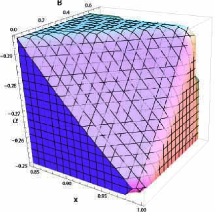
Figure 5: Three-dimensional plot of the inequality in eq.(27) in terms of the pair of parameters (i.e. $\alpha,\,B$) and the dimensionless $x$ variable.

V Conclusions

In this paper we investigated the constraints imposed by the GSL on modified Friedmann equations that arise from quantum corrections to the entropy-area relation, eq. (1). As is well known, the GSL is a powerful tool to set bounds on astrophysical and cosmological models -see e.g. paul ; macgibbon ; chimento ; izquierdo .

Cosmological equations follow either from Jacobson’s approach, that connects gravity to thermodynamics by associating Einstein equations to Clausius relation (6), or Padmanabhan’s suggestion that relates gravity (i.e., Einstein equations) to microscopic degrees of freedom through the principle of equipartition of energy (2). We analyzed two entropy-area terms, logarithmic (3), and power-law corrections (4), the former coming from loop quantum gravity, the latter from the entanglement of quantum fields.

Both quantum corrections have been widely investigated but, since they come from very different techniques, one should not be surprised that total agreement on these corrections is still missing. In particular, there is a lack of consensus on the value of the constant parameter $\alpha$. Our work aimed to discriminate among quantum corrections by requiring, via a classical analysis, the GSL to be fulfilled throughout the evolution of the Universe. This sets constraints on the value of the parameter.

We first investigated the intervals of values of $\alpha$ compatible with the GSL by assuming that the DEC holds true for the perfect fluid that sources the gravitational field of the FRW universe. In the case of logarithmic corrections to the horizon entropy this gives a wide range, in which positive values are largely favored, with no upper bound in the case of the modified Friedmann equation derived from Clausius relation. Negative values of $\alpha$ are consistent with the GSL only up to $\alpha=-1/4$, hence discarding two negative values that have been suggested in the literature, namely, $\alpha=-1/2$ ghosh04 , and $\alpha=-3/2$ kaul00 .
In the case of power-law entropy corrections, our analysis favors positive values of $\alpha$, though they are expected to be negative. Only a small concordance range appears when modified Friedmann equations from the equipartition of energy are employed. Specifically, the interval $3<\alpha<4$ corresponds to a power-law correction with an index between $-1$ and 0, that has been analytically or numerically obtained saurya08 ; jacobson93 .

The second part of our analysis considered the possibility of enlarging the allowed interval of $\alpha$ in the case of logarithmic entropy corrections by considering either a phantom phase for the fluid or particle production modelled as an effective bulk viscosity. Phantom behavior affects positive values of $\alpha$ while particle production could enlarge the negative range and incorporate the value $\alpha=-1/2$ that seems widely accepted in literature ghosh04 .

- (1) J.D. Bekenstein, Black holes and entropy, Phys. Rev. D, 7:2333–2346, 1973.
- (2) P.C.W. Davies, Scalar production in Schwarzschild and Rindler metrics, J. Phys. A, 8:609, 1973.
- (3) G.W. Gibbons and S.W. Hawking, Cosmological event horizons, thermodynamics, and particle creation, Phys. Rev. D, 15:2738–2751, 1977.
- (4) Guo-Hong Yang Shao-Feng Wu, Bin Wang, Thermodynamics on the apparent horizon in generalized gravity theories, Nucl.Phys.B, 799:330–344, 2008.
- (5) Shao-Feng Wu, Bin Wang, Guo-Hong Yang, and Peng-Ming Zhang, The generalized second law of thermodynamics in generalized gravity theories, Class.Quant.Grav., 25:235018, 2008.
- (6) Rong-Gen Cai, Li-Ming Cao, and Ya-Peng . Hu, Hawking radiation of apparent horizon in a FRW universe, Class. Quantum Grav., 26:155018, 2009.
- (7) T. Jacobson, Thermodynamics of space-time: The Einstein equation of state, Phys. Rev. Lett., 75:1260, 1995.
- (8) T. Padmanabhan, Surface density of spacetime degrees of freedom from equipartition law in theories of gravity, arXiv:1003.5665v1 [gr-qc], 2010.
- (9) T. Padmanabhan, Entropy of null surfaces and dynamics of spacetime, Phys.Rev. D, 75:064004, 2008.
- (10) K. A. Meissner, Black hole entropy from loop quantum gravity, Class. Quantum Grav., 21:5245–5252, 2004.
- (11) A. Ghosh and P. Mitra, On the log correction to the black hole area law, Phys. Rev. D, 71:027502, 2004.
- (12) Ashok Chatterjee and Parthasarathi Majumdar, Universal canonical black hole entropy, Phys. Rev. Lett., 92:141301, 2004.
- (13) Saurya Das, S. Shankaranarayanan, and Sourav Sur, Power-law corrections to entanglement entropy of horizons, Phys. Rev. D, 77:064013, 2008.
- (14) J.E. Lidsey, Thermodynamics of anomaly-driven cosmology, Class. Quantum Grav., 26:147001, 2009.
- (15) Yi Zhang, Yun-gui Gong, and Zong-Hong Zhu, Modified gravity emerging from thermodynamics and holographic principle, arXiv:1001.4677v1 [hep-th], 2010.
- (16) J.D. Bekenstein, Generalized second law of thermodynamics in black-hole physics, Phys. Rev. D, 9:3292, 1974.
- (17) T. Padmanabhan, Thermodynamical aspects of gravity: New insights, Rep. Prog. Phys., 73:046901, 2010.
- (18) P.C.W. Davies, Cosmological horizons and the generalised second law of thermodynamics, Class. Quantum Grav., 4:L225, 1987.
- (19) S. Hod, High-order corrections to the entropy and area of quantum black holes, Class. Quantum Grav., 21:L97, 2004.
- (20) G.R. Dvali and M.S. Turner, Dark energy as a modification of the Friedmann equation, arXiv:astro-ph/0301510v1, 2003.
- (21) Ya. B Zel’Dovich, Particle production in cosmology, JETP Lett., 12:307, 1970.
- (22) B.L. Hu, Vacuum viscosity description of quantum processes in the early universe, Phys. Lett. A, 90:375, 1982.
- (23) J.D. Barrow, String-driven inflationary and deflationary cosmological models, Nucl. Phys. B, 310:743, 1988.
- (24) W Zimdahl and D. Pavón, Cosmology with adiabatic matter creation, Phys. Lett. A, 176:57, 1993.
- (25) M.O. Calvão, J.A. Lima, and I. Waga, On the thermodynamics of matter creation in cosmology, Phys. Lett. A, 162:223, 1992.
- (26) M. Domagala and J. Lewandowski, Black hole entropy from quantum geometry, Class. Quantum Grav., 21:5233–5244, 2004.
- (27) P.C.W. Davies, T.M. Davis, and C.H. Lineweaver, Cosmology: Black holes constrain varying constants, Nature, 418:602, 2002.
- (28) J.H. MacGibbon, Black hole constraints in varying fundamental constants, Phys. Rev. Lett., 99:061301, 2007.
- (29) L.P. Chimento, Jakubi, A.S., and D. Pavón, Varying c and particle horizons, Phys. Lett. B, 508:1, 2001.
- (30) G. Izquierdo and D. Pavón, Dark energy and the generalized second law, Phys. Lett. B, 633:420, 2006.
- (31) R.K. Kaul and P. Majumdar, Logarithmic correction to the Bekenstein-Hawking entropy, Phys. Rev. Lett., 84:5255, 2000.
- (32) T. Jacobson and R.C. Myers, Black hole entropy and higher curvature interactions, Phys. Rev. Lett., 70:3683, 1993.