Exact solutions of the Gross-Pitaevskii equation for stable vortex modes

Abstract

We construct exact solutions of the Gross-Pitaevskii equation for solitary vortices, and approximate ones for fundamental solitons, in 2D models of Bose-Einstein condensates with a spatially modulated nonlinearity of either sign and a harmonic trapping potential. The number of vortex-soliton (VS) modes is determined by the discrete energy spectrum of a related linear Schrödinger equation. The VS families in the system with the attractive and repulsive nonlinearity are mutually complementary. Stable VSs with vorticity $S\geq 2$ and those corresponding to higher-order radial states are reported for the first time, in the case of the attraction and repulsion, respectively.

The realization of Bose-Einstein condensates (BECs) in dilute quantum gases has drawn a great deal of interest to the dynamics of nonlinear excitations in matter waves, such as dark dark and bright solitons bright , vortices vortex ; BECvortex , supervortices supervortex , etc. The work in this direction was strongly stimulated by many similarities to solitons and vortices in optics optics . In the mean-field approximation, the BEC dynamics at ultra-low temperatures is accurately described by the Gross-Pitaevskii equation (GPE), the nonlinearity being determined by the $s$-wave scattering length of interatomic collisions, which can be controlled by means of the magnetic magnetic or low-loss optical optical Feshbach-resonance technique, making spatiotemporal “management” of the local nonlinearity possible through the use of time-dependent and/or non-uniform fields optics . In particular, a recently developed technique, which allows one to “paint” arbitrary one- and two-dimensional (1D and 2D) average patterns by a rapidly moving laser beam painting , suggests new perspectives for the application of the nonlinearity management based on the optical Feshbach-resonance. A counterpart of the GPE, which is a basic model in nonlinear optics, is the nonlinear Schrödinger equation (NLSE) optics . In the latter case, the modulation of the local nonlinearity can be implemented too–in particular, by means of indiffusion of a dopant resonantly interacting with the light.

The search for exact solutions to the GPE/NLSE is an essential direction in the studies of nonlinear matter and photonic waves. In particular, stable soliton solutions are of great significance to experiments and potential applications, as they precisely predict conditions which should allow the creation of matter-wave and optical solitons, including challenging situations which have not yet been tackled in the experiment, such as 2D matter-wave solitons and solitary vortices review . In the 1D setting with the spatially uniform nonlinearity, exact stable solutions for bright and dark solitons have been constructed in special cases, when the external potential is linear or quadratic homogeneous , and a specially designed inhomogeneous nonlinearity may support bound states of an arbitrary number of solitons beitia . In the 2D geometry with the uniform nonlinearity, exact delocalized solutions were constructed in the presence of a periodic potential LDcarr2 . In the 2D geometry, 1D bright and dark solitons are unstable, with the bright ones suffering the breakup into a chain of collapsing pulses, and the dark solitons splitting into vortex-antivortex pairs dark ; RDS . Another approach to finding exact solitonic states in both 1D and 2D settings (with the uniform nonlinearity), along with the supporting potentials, was proposed in the form the respective inverse problem Step . As concerns vortices, while delocalized ones have been created and extensively investigated in self-repulsive BECs vortex , and vortex solitons (VSs) were created in photorefractive crystals equipped with photonic lattices photorefr , analytical solutions for localized vortices have not been reported yet, and experimental creation of stable VSs in self-attractive BEC and optical media with the fundamental cubic nonlinearity remains a challenge to the experiment.

In this work we demonstrate that exact VS solutions can be found in the 2D GPE/NLSE, with a specially designed (and experimentally realizable) profile of the radial modulation of the nonlinearity coefficient, of both attractive and repulsive types. In fact, the search for localized solutions in 2D models with diverse nonlinearity-modulation profiles has recently attracted considerable attention 2D , although no exact solutions have been reported. We consider only nonlinearity-modulation patterns which do not change the sign, as zero-crossing would make the use of the FR problematic magnetic ; optical .

The scaled form of the GPE/NLSE is $i{\psi}_{t}=-\nabla^{2}\psi+g(r)|\psi|^{2}\psi+V(r)\psi$, where $\psi$ is the BEC macroscopic wave function, $\nabla^{2}$ the 2D Laplacian, and $g(r)$ is the nonlinearity coefficient which, as well as external potential $V(r)$, is a function of radial coordinate $r$. The same equation finds a straightforward implementation as a spatial-domain model of the beam propagation in bulk media, with $t$, $\psi$, and $g(r)$ being the propagation distance, amplitude of the electromagnetic field, and the local Kerr coefficient.

Assuming the stationary wave function as $\psi(r,\theta,t)=\phi(r)\exp(iS\theta-i\mu t)$, where $\theta$ is the azimuthal angle, $S$ an integer vorticity, and $\mu$ the chemical potential (or propagation constant in optics), leads to the equation for the real stationary wave function $\phi(r)$: $\mu\phi=-\phi^{\prime\prime}-r^{-1}\phi^{\prime}+g(r)\phi^{3}+\left[{S^{2}r^{-2}+}V(r)\right]\phi$. For $S\neq 0$, $\phi(r)$ should vary as $r^{|S|}$ at $r\rightarrow 0$, which is replaced by $\phi^{\prime}(r=0)=0$ for $S=0$. The localization requires $\phi(r=\infty)=0$.

Defining $\phi(r)\equiv\rho(r)U(R(r))$, $g(r)\equiv g_{0}r^{-2}\rho^{-6}(r)$, with $R(r)\equiv\int_{0}^{r}s^{-1}\rho^{-2}(s)ds$, one can find that $\rho(r)$ and $U(R)$ obey the following equations:

$$\rho^{\prime\prime}+r^{-1}\rho^{\prime}+\left(\mu-V(r)-S^{2}r^{-2}\right)\rho =Er^{-2}\rho^{-3},$$ (1)

$$-d^{2}U/dR^{2}+g_{0}U^{3} =EU,$$ (2)

where $E$ and $g_{0}$ are constants. The reduction of the GPE/NLSE to Eq. (2) helps one to find exact solutions, as the latter equation is solvable in terms of elliptic functions. Then, if a solution to Eq. (1) is known, one can construct exact solutions to the underlying GPE/NLSE, while the nonlinearity-modulation profile admitting exact solutions is determined by $\rho(r)$. Physical solutions impose restrictions on $\rho$: from expressions for $R(r)$ and $g(r)$ it follows that $\rho$ cannot change its sign; further, it must behave as $r^{-a}$ with $a\geq 1/3$ at $r\rightarrow 0$, and diverge ($\rho\rightarrow\infty$) at $r\rightarrow\infty$, so that the nonlinearity strength is bounded and the integration in $R(r)$ converges.

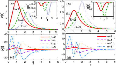
Figure 1: (Color online). (a) Exact vortex solitons without the external potential. Inset, the corresponding profiles of the attractive-nonlinearity coefficient. (c) Exact vortex solitons of different radial quantum number $n$ with $S=1$, the respective nonlinearity-coefficient profile being depicted by the solid line in the inset of (a). Parameters are $c_{3,4}=-\mu=-g_{0}=1$. (b) and (d): The same as (a) and (c) when the trapping potential is present, $V=0.01r^{2}$, with $c_{1,2}=3$.

We begin constructing exact VS solutions for the attractive nonlinearity ($g_{0}<0$) when $E=0$, so that Eq. (1) is solvable. With the harmonic potential $V=kr^{2}$, $\rho$ can be found in terms of the Whittaker’s $\mathrm{M}$ and $\mathrm{W}$ functions whittaker : $\rho(r)=r^{-1}[c_{1}\mathrm{M}({\mu}/{4\sqrt{k}},{|S|}/{2},\sqrt{k}r^{2})+c_{2}\mathrm{W}({\mu}/{4\sqrt{k}},{|S|}/{2},\sqrt{k}r^{2})]$, where the restrictions on $\rho$ require $\mu<\mu_{0}=2(1+|S|)\sqrt{k}$ and $c_{1}c_{2}>0$. Without the trap ($k=0$), $\rho$ degenerates to $\rho(r)=c_{3}I_{S}(\sqrt{-\mu}r)+c_{4}K_{S}(\sqrt{-\mu}r)$, with $\mu<\mu_{0}=0$, $I_{S}$ and $K_{S}$ being the modified Bessel and Hankel functions, and the constants satisfying $c_{3}c_{4}>0$. In both cases, one has $\rho(r)\sim r^{-|S|}$ at $r\rightarrow 0$, hence $g(r)\sim r^{6|S|-2}$ and $R(r)\sim r^{2|S|}$ at $r\rightarrow 0$, and $\rho(r)\rightarrow\infty$ as $r\rightarrow\infty$. Thus, the respective nonlinearity is localized and bounded, and $R(r)$ is bounded too. To meet boundary conditions $\phi(0)=\phi(\infty)=0$, an exact solution to Eq. (2) is chosen as

$$U(R)=\left(n\eta/\sqrt{-g_{0}}\right)\mathrm{cn}\left(n\eta R-K(1/\sqrt{2}),1/\sqrt{2}\right),$$ (3)

where $n=2,4,6,\cdots$ with $n/2$ being the radial quantum number, $\eta\equiv K(\sqrt{2}/2)/R(r=\infty)$, and $K(1/\sqrt{2})$ is the complete elliptic integral of the first kind.

It follows from Eq. (3) that $U(R)\sim R$ at $R\rightarrow 0$, which implies that the amplitude of the exact VS is $\rho U\sim r^{|S|}$ at $r\rightarrow 0$, as it should be. Thus, for given $\mu$, $S$, and nonlinearity strength $g_{0}$ (and $k$, in the presence of the trap), one can construct an infinite number of exact VSs with $n/2$ bright rings surrounding the vortex core, as shown in Fig. 1. Although these VSs share the same chemical potential, their energies increase with the increase of even number $n$.

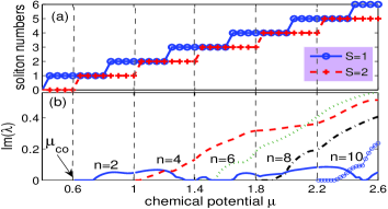
Figure 2: (Color online). (a) The number of numerically found vortex-soliton modes versus the chemical potential in the case of the repulsive nonlinearity, with the harmonic trap. (b) The largest instability growth rate for numerically found vortices with $S=2$, $E=1$ and $k=0.01$.

Next we consider the repulsive nonlinearity, $g_{0}>0$, and include the harmonic trap to confine the system. In this case, the existence of elliptic-function solutions to Eq. (2) requires $E>0$, hence Eq. (1) is a nonlinear equation, which can be solved only in a numerical form. To construct the VSs in this case, one requires $\rho\sim r^{-|S|}$ (for $S\neq 0$) at $r\rightarrow 0$, hence the nonlinear term in Eq. (1) may be neglected near $r=0$. Thus, $\rho$ is similar to the Neumann function, $Y_{S}(\sqrt{\mu}r)$, at $r\rightarrow 0$ for $\mu>0$ (for $\mu<0$ it can be checked that VS solutions do not exist). On the other hand, $\rho\rightarrow\infty$ at $r\rightarrow\infty$, due to the the presence of the harmonic trap. Further, term $Er^{-2}\rho^{-3}$ with $E>0$ in Eq. (1) guarantees the sign-definiteness of $\rho(r)$. Therefore, taking small $r_{0}$ as an initial point and using the Neumann function and its derivative at $r=r_{0}$ as initial conditions, one can numerically integrate Eq. (1) to obtain $R(r)$ and $g(r)$; then VSs can be constructed in the numerical form, using the exact solution to Eq. (2),

$$U(R)=\sqrt{{2(E-B^{2})}/{g_{0}}}\mathrm{sn}\left(BR,\sqrt{{E}/{B^{2}}-1}\right),$$ (4)

subject to a constraint with even numbers $n$,

$$\sqrt{{E}/{2}}<B\equiv n{K(\sqrt{E/B^{2}-1})}/{R(\infty)}<\sqrt{E}.$$ (5)

From Eq. (5) it follows that $n<n_{\max}=2R(\infty)\sqrt{E}/\pi$. This implies that there is a finite number of the VS modes (or none, if $n_{\max}<2$), in contrast to the case of the attractive nonlinearity, where the infinite set of exact VSs was constructed. Figure 2(a) shows the number of the numerical VS solutions versus $\mu$, demonstrating that the cutoff value of the chemical potential is same as for the exact VSs with the attractive nonlinearity, and the number of VSs jumps at points $\mu=\mu_{j}^{(S)}\equiv 2(2j+|S|-1)\sqrt{k}$, with $j=1,2,3,\cdots$, which is precisely the $j$-th energy eigenvalue of the vortex state in the corresponding linear Schrödinger equation. Thus, there are $j$ numerically exact VSs, associated with expression (4), where $n=2,4,6,\cdots,2j$, in interval $\mu_{j}^{(S)}<\mu\leq\mu_{j+1}^{(S)}$. A similar result is true for the 1D GPE with the optical-lattice potential, where $n$ families of fundamental gap solitons exist in the $n$-th bandgap wubiao . Figure 3 displays a characteristic example of the numerically found VSs, in the case when four of them exist. Similarly, it can be shown that there are infinitely many VSs, but just the first $j$ modes do not exist, when $\mu_{j}^{S}\leq\mu<\mu_{j+1}^{S}$ for the attractive nonlinearity, which demonstrates that the repulsive and attractive nonlinearities are mutually complementary ones, in this respect.

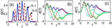
Figure 3: (Color online). (a) Modulation profiles of the repulsive nonlinearity for numerically found vortices, which are displayed in (b) for $S=1$ and in (c) for $S=2$, in the presence of the harmonic trap. Opened circles, squares, solid circles, and triangles denote solutions with $n=2$, 4, 6, and 8, respectively. Parameters are $E=1$, $\mu=2$, $k=g_{0}=0.01$.

Solutions can also be found for 2D fundamental solitons ($S=0$) supported by the following two-tier nonlinearity, with constant $g_{r}$:

$$g(r)=g_{r}~{}(\mathrm{at}~{}0\leq r<r_{0}),~{}{g_{0}}{\rho^{-6}r^{-2}}\ \left(\mathrm{at}~{}r\geq r_{0}\right).$$ (6)

For $r\geq r_{0}$, exact solutions can be found in the same way as above, except that now $R(r)\equiv\int_{r_{0}}^{r}ds/[s\left(\rho(s)\right)^{2}]$. At $r<r_{0}$, if $r_{0}$ is small in comparison with the spatial scale of the external potential (for instance, $r_{0}\ll\sqrt{1/k}$, in the presence of $V=kr^{2}$), $\phi(r)$ may be approximated by a constant, $\phi=\sqrt{[\mu-V(0)]/g_{r}}$. Because $\phi(r)$ and $\phi^{\prime}(r)$ must be continuous at $r=r_{0}$, one then requires $\rho^{\prime}(r_{0})=0$ and $dU(0)/dR=0$, which leads to $g_{r}=[\mu-V(0)]\left[\rho(r_{0})U(0)\right]^{-2}$. In this case, the solution to Eq. (2) is given by Eqs. (4) and (5), with $BR$ replaced by $BR+K(\sqrt{E/B^{2}-1})$, and $n=1,3,5,\cdots$ for the repulsive nonlinearity, to make $\phi(\infty)=0$. Similar solutions can be constructed for the attractive nonlinearity. Examples of the fundamental solutions are presented in Fig. 4.

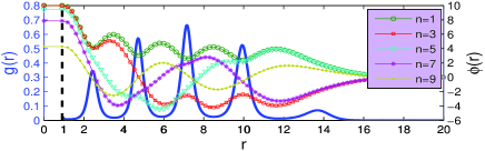
Figure 4: (Color online). Fundamental solitons supported by the repulsive two-tier nonlinearity, see Eq. (6). The constant values of $g_{r}$ for $n=1,3,5,7$ and 9 are respectively $0.0200,0.0201,0.0224,0.0325$, and 0.1093. Parameters are $\rho(r_{0})=1$, $\rho^{\prime}(r_{0})=0$, $r_{0}=E=1$, $k=g_{0}=0.01$, $\mu=2$.

We employed the linear stability analysis and direct simulations to verify the stability of the solitons. For the attractive nonlinearity, we have found that all exact VSs are subject to the azimuthal modulational instability without the external potential. As a result, the VSs break up, and eventually collapse. However, the lowest-order exact VSs with $n=2$ are stable in the presence of the harmonic trap, if $\mu$ is close enough to the cutoff value $\mu_{0}$, while the amplitude of the VS does not become small, see Fig. 5. We stress that, in numerous previous works, a stability region for VSs trapped in the harmonic potential was found solely for $S=1$, all vortices with $S\geq 2$ being conjectured unstable BECvortex . The present results report the first example of stable vortices with $S\geq 2$ in the trapped self-attractive fields.

In the case of the repulsive nonlinearity combined with the harmonic trap, the numerically found VSs can be stable for every $n$ at which they exist, within some region of values of $\mu$, see Fig. 2(b). This finding is remarkable in the sense that previous works did not report stable trapped vortices in higher-order radial states. Moreover, Figs. 2(b) and 6 demonstrates that VSs with the largest number of rings may be more stable than its counterparts with fewer rings. An explanation to this feature is that local density peaks place themselves in troughs of the nonlinearity landscape, thus lowering the system’s energy. Similar properties are featured by the fundamental solitons. Numerical simulations show that those VSs with $n=2$ which are unstable either split into vortices with lower topological charges or exhibit a quasi-stability, periodically breaking and recovering the axial symmetry [Fig. 6(a)], similar to what was previously observed in the case of the attractive nonlinearity BECvortex ; stable , while unstable VSs with $n=4,6,\cdots$ ultimately evolve into vortices located close to zero-amplitude points.

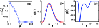
Figure 5: (Color online). (a) The largest instability growth rate for exact vortex solitons with $S=3$ and the attractive nonlinearity. (b) A stable vortex (solid lines, with circles showing its profile at $t=200$, when it was initially perturbed by random noise), and (c) the corresponding nonlinearity coefficient when $\mu=0.7$. Here $g_{0}=-1000$, $k=0.01$, and $c_{1,2}=3$.

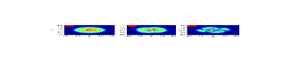
Figure 6: (color online). (a) The result of the quasi-stable evolution of a numerically found vortex with $n=2$, in the case of the self-repulsion, at $t=1700$. (b, c) Unstable vortices with $n=4$ and $6$ at $t=60$ and $70$, respectively. Parameters are $S=2$, $E=1$, $g_{0}=k=0.01$, $\mu=1.82$. The vortex with $n=8$ are stable.

In conclusion, we have constructed exact solutions of the Gross-Pitaevskii equation for solitary vortices, and approximate ones for fundamental solitons in the framework of the GPE/NLSE with 2D axisymmetric profiles of the modulation of the nonlinearity coefficient, and harmonic trapping potential. We have demonstrated that the attractive/repulsive nonlinearity supports an infinite/finite number of exact VSs. In particular, stable VSs with vorticity $S\geq 2$, as well as those corresponding to higher-order radial states, have been produced for the first time. The results suggest a scenario for the creation of stable vortex solitons in BEC and optics, which have not been as yet observed in experiments. The necessary BEC nonlinearity landscape can be built by means of the Feshbach-resonance technique. The corresponding nonuniform magnetic field may be created by a micro-fabricated ferromagnetic structure integrated into the matter-wave chip exper , or one can use the respective pattern of the laser beams. In optics, the same nonlinearity landscape may created by a nonuniform distribution of nonlinearity-enhancing dopants. The method developed in this work for finding the exact solutions, which is based on reducing the 2D equation to the solvable system of Eqs. (1) and (2), can be applied to other models. In particular, a challenging problem is to devise a physically relevant model admitting exact 3D solitons.

This work was supported by the NNSF of China (Grants No. 10672147, 10704049 and 10934010), the NKBRSFC (Grant No. 2006CB921400), PNSF of Shanxi (Grant No. 2007011007), and the German-Israeli Foundation through grant No. 149/2006.

References

- (1) S. Burger et al., Phys. Rev. Lett. 83, 5198 (1999); J. Denschlag et al., Science 287, 97 (2000); B. P. Anderson et al., Phys. Rev. Lett. 86, 2926 (2001).
- (2) K. E. Strecker et al., Nature 417, 150 (2002); L. Khaykovich et al., Science 296, 1290 (2002).
- (3) M. R. Matthews et al., Phys. Rev. Lett. 83, 2498 (1999); K. W. Madison et al., ibid. 84, 806 (2000); S. Inouye et al., ibid. 87, 080402 (2001); J. R. Abo-Shaeer, et al. Science 292, 476 (2001); A. L. Fetter, Rev. Mod. Phys. 81, 647 (2009).
- (4) T. J. Alexander and L. Bergé, Phys. Rev. E 65, 026611 (2002); D. Mihalache et al., Phys. Rev. A 73, 043615 (2006); L. D. Carr and C. W. Clark, Phys. Rev. Lett. 97, 010403 (2006).
- (5) H. Sakaguchi and B. A. Malomed, Europhys. Lett. 72, 698 (2005).
- (6) Y. S. Kivshar and G. P. Agrawal, Optical Solitons: from Fibers to Photonic Crystals (Academic Press: San Diego, 2003); B. A. Malomed, Soliton Management in Periodic Systems (Springer: New York, 2006).
- (7) A. J. Moerdijk et al., Phys. Rev. A51, 4852 (1995); J. L. Roberts et al., Phys. Rev. Lett. 81, 5109 (1998); S. L. Cornish et al., ibid. 85, 1795 (2000).
- (8) M. Theis et al., Phys. Rev. Lett. 93, 123001 (2004); R. Ciurylo et al., Phys. Rev. A 71, 030701(R) (2005); K. Enomoto et al., Phys. Rev. Lett. 101, 203201 (2008); Y. N. Martinez de Escobar et al., ibid. 103, 200402 (2009).
- (9) K. Henderson et al., New J. Phys. 11, 043030 (2009).
- (10) B. A. Malomed, D. Mihalache, F. Wise, and L. Torner, J. Optics B: Quant. Semicl. Opt. 7, R53 (2005).
- (11) H. H. Chen and C. S. Liu, Phys. Rev. Lett. 37, 693 (1976); V. N. Serkin et al., ibid. 98, 074102 (2007); V. N. Serkin and A. Hasegawa, ibid. 85, 4502 (2000); Z. X. Liang et al., ibid. 94, 050402 (2005).
- (12) J. Belmonte-Beitia, V. M. Pérez-García, and V. Vekslerchik, Phys. Rev. Lett. 98, 064102 (2007); J. Belmonte-Beitia et al., ibid. 100, 164102 (2008).
- (13) R. M. Bradley et al., Phys. Rev. A77, 033622 (2008).
- (14) G. Theocharis et al., Phys. Rev. Lett. 90, 120403 (2003).
- (15) B. A. Malomed and Yu. A. Stepanyants, Chaos 20, 013130 (2010); Y. Wang and R. Hao, Opt. Commun. 282, 3995 (2009).
- (16) D. N. Neshev et al., Phys. Rev. Lett. 92, 123903 (2004); J. W. Fleischer et al, ibid. 92, 123904 (2004).
- (17) Y. Sivan, G. Fibich, and M. I. Weinstein, Phys. Rev. Lett. 97, 193902 (2006); H. Sakaguchi and B. A. Malomed, Phys. Rev. E 73, 026601 (2006); ibid. 75, 063825 (2007); Y. Sivan et al., ibid. 78, 046602 (2008); Y. V. Kartashov et al., Opt. Lett. 33, 1747 (2008); ibid. 33, 2173 (2008); ibid. 34, 770 (2009); C. Hang, V. V. Konotop, and G. Huang, Phys. Rev. A 79, 033826 (2009); D. Wang et al., Phys. Rev. A81, 025604 (2010).
- (18) E. T. Whittaker and G. N. Watson, A Course in Modern Analysis, 4th ed. (Cambridge University Press, Cambridge, UK, 1990).
- (19) Y. Zhang and B. Wu, Phys. Rev. Lett. 102, 093905 (2009).
- (20) B. LeMesurier and P. Christiansen, Physica D 184, 226 (2003).
- (21) M. Vengalattore et al., J. Appl. Phys. 95, 4404 (2004); Eur. Phys. J. D 35, 69 (2005).