Shape mixing dynamics in the low-lying states of proton-rich Kr isotopes

Abstract

We study the oblate-prolate shape mixing in the low-lying states of proton-rich Kr isotopes using the five-dimensional quadrupole collective Hamiltonian. The collective Hamiltonian is derived microscopically by means of the CHFB (constrained Hartree-Fock-Bogoliubov) + Local QRPA (quasiparticle random phase approximation) method, which we have developed recently on the basis of the adiabatic self-consistent collective coordinate method. The results of the numerical calculation show the importance of large-amplitude collective vibrations in the triaxial shape degree of freedom and rotational effects on the oblate-prolate shape mixing dynamics in the low-lying states of these isotopes.

1 Introduction

Atomic nuclei exhibit different shapes depending on the numbers of proton and neutron, the excitation energies, or angular momentum. Shape coexistence phenomena, in which an excited band with a shape different from the shape in the ground band exists close to the ground band, are widely observed all over the nuclear chart. From the mean-field viewpoint, shape coexistence indicates that there are two equilibrium points in the mean field, and appearance of a low-lying excited $0^{+}$ state is one of typical indications of the shape coexistence.

In proton-rich Kr isotopes, it has been conjectured that the oblate and prolate shapes coexist in their low-lying states, since the ground bands quite different from regular rotational spectra [1, 2] and the low-lying excited $0^{+}$ states [3, 4] were measured. Since then, much experimental data have been accumulated for proton-rich Kr isotopes [5, 6, 7, 8] and they support the interpretation as the oblate-prolate shape coexistence. The spectroscopic quadrupole moments [6] suggest the prolate ground state in ⁷⁴Kr and ⁷⁶Kr, while the ground state of ⁷²Kr is assumed to be oblate from the properties of the $E2$ transition probabilities [7]. The systematics of the electric monopole transition strengths [3, 4, 9] and the excitation energies of the first excited $0^{+}$ states are consistent with the interpretation that a shape transition from the oblate ground state in ⁷²Kr to the prolate ground states in ⁷⁴Kr and ⁷⁶Kr takes place.

The description of these isotopes can be a touchstone for nuclear structure models, and many attempts were done from several theoretical approaches [10, 11, 12, 13, 14, 15, 16]. Recently Girod et al. [17] have reproduced the shape transition from the oblate ground state in ⁷²Kr to the prolate in ⁷⁶Kr with the HFB (Hartree-Fock-Bogoliubov)-based GCM (generator coordinate method) + GOA (Gaussian overlap approximation) calculation. Making a comparison with the result of the axial GCM calculation done by Bender et al. [15], they have pointed out that the triaxial shape plays an essential role in the shape coexistence and the shape transition in the light Kr isotopes. The importance of large-amplitude collective vibrations in the triaxial shape degree of freedom has also been shown in the previous works for ⁷²Kr [18] and neighboring ^68-72Se [19] on the basis of the (1+3) dimensional calculation using the adiabatic self-consistent collective coordinate (ASCC) method [20, 21].

In this paper, we study the low-lying states of proton-rich Kr isotopes using a new method we have developed recently [22]. In this method, we determine the five-dimensional (5D) quadrupole collective Hamiltonian [23, 24, 25, 26] microscopically on the basis of the ASCC method. Local normal modes on top of each constrained HFB (CHFB) state at each point on the ($\beta,\gamma$) plane is the main concept. After solving the CHFB equations imposing the constraints on the deformation and the particle numbers, we solve the local QRPA (LQRPA) equations, which is an extension of the usual QRPA (quasiparticle random phase approximation) to non-HFB-equilibrium points, on top of the CHFB states. Therefore, we call this method the CHFB+LQRPA method. Using this method, we derive the seven quantities in the collective Hamiltonian: the collective potential, three vibrational inertial masses, and three rotational moments of inertia.

One of the advantages of the CHFB+LQRPA method is that the vibrational and rotational masses (inertial functions) determined with this method contain the contributions from the time-odd components of the mean-field unlike the widely-used Inglis-Belyaev (IB) cranking masses [27, 28]. It is well known that the ignorance of the time-odd components in the IB masses breaks the self-consistency of the theory [29, 30]. Nevertheless, even in recent microscopic studies by means of the 5D quadrupole collective Hamiltonian [17, 31, 32, 33, 34], the IB cranking masses are still used at least for vibrational inertial functions. In this study, we use the pairing-plus-quadrupole (P+Q) force model [35, 36] including the quadrupole-pairing force and take into account the contributions from the time-odd components of the mean field to the vibrational and rotational masses. Inclusion of the quadrupole pairing force is essential because it is the only term which gives the time-odd components of the mean field [37].

This paper is organized as follows. In Section 2, we summarize the procedure of deriving the 5D quadrupole collective Hamiltonian by means of the CHFB+LQRPA method. In Section 3, we calculate the vibrational and rotational masses. By solving the collective Schrödinger equation, we calculate excitation spectra, $B(E2)$, spectroscopic quadrupole moments and monopole transition matrix elements for the low-lying states in ^72,74,76Kr and discuss the properties of the oblate-prolate shape coexistence/mixing in these nuclei. Conclusion is given in Section 4.

2 Microscopic derivation of the 5D quadrupole collective Hamiltonian

In this section, we summarize the procedure of microscopically deriving the 5D quadrupole collective Hamiltonian and the collective Schrödinger equation by means of the CHFB+LQRPA method.

2.1 5D quadrupole Hamiltonian and collective Schrödinger equation

The 5D quadrupole collective Hamiltonian is written in terms of the magnitude $\beta$ and the degree of triaxiality $\gamma$ of quadrupole deformation, and their time derivatives, $\dot{\beta}$ and $\dot{\gamma}$, as

$${\cal H}_{\rm coll} =T_{\rm vib}+T_{\rm rot}+V(\beta,\gamma),$$ (1)

$$T_{\rm vib} =\frac{1}{2}D_{\beta\beta}(\beta,\gamma)\dot{\beta}^{2}+D_{\beta\gamma}(\beta,\gamma)\dot{\beta}\dot{\gamma}+\frac{1}{2}D_{\gamma\gamma}(\beta,\gamma)\dot{\gamma}^{2},$$ (2)

$$T_{\rm rot} =\frac{1}{2}\sum_{k=1}^{3}{\cal J}_{k}(\beta,\gamma)\omega^{2}_{k},,$$ (3)

where $T_{\rm vib}$, $T_{\rm rot}$ and $V$ represent the vibrational, rotational and collective potential energies, respectively. The 5D quadrupole collective Hamiltonian has seven quantities to be determined: three vibrational inertial masses, three rotational moments of inertia, and the collective potential. The moments of inertia can be parametrized as

$${\cal J}_{k}(\beta,\gamma)=4\beta^{2}D_{k}(\beta,\gamma)\sin^{2}\gamma_{k}\quad(k=1,2,3)$$ (4)

with $\gamma_{k}=\gamma-(2\pi k/3)$. The vibrational and rotational masses are, in general, functions of the deformation parameters. How to determine these inertial masses and the collective potential is discussed in the following subsection.

As the collective Hamiltonian (1) is classical, we quantize it according to the Pauli prescription to obtain the collective Schrödinger equation

$$\{\hat{T}_{\rm vib}+\hat{T}_{\rm rot}+V\}\Psi_{\alpha IM}(\beta,\gamma,\Omega)=E_{\alpha I}\Psi_{\alpha IM}(\beta,\gamma,\Omega),$$ (5)

where

$$\hat{T}_{\rm vib}=\frac{-1}{2\sqrt{WR}}\left\{\frac{1}{\beta^{4}}\left[\left(\partial_{\beta}\beta^{2}\sqrt{\frac{R}{W}}D_{\gamma\gamma}\partial_{\beta}\right)-\partial_{\beta}\left(\beta^{2}\sqrt{\frac{R}{W}}D_{\beta\gamma}\partial_{\gamma}\right)\right]\right.$$ (6)

$$\left.+\frac{1}{\beta^{2}\sin 3\gamma}\left[-\partial_{\gamma}\left(\sqrt{\frac{R}{W}}\sin 3\gamma D_{\beta\gamma}\partial_{\beta}\right)+\partial_{\gamma}\left(\sqrt{\frac{R}{W}}\sin 3\gamma D_{\beta\beta}\partial_{\gamma}\right)\right]\right\}$$ (7)

and

$$\hat{T}_{\rm rot}=\sum_{k}\frac{\hat{I}_{k}^{2}}{2{\cal J}_{k}}.$$ (8)

Here, $R(\beta,\gamma)$ and $W(\beta,\gamma)$ are defined as

$$R(\beta,\gamma)= D_{1}(\beta,\gamma)D_{2}(\beta,\gamma)D_{3}(\beta,\gamma),$$ (9)

$$W(\beta,\gamma)= \left\{D_{\beta\beta}(\beta,\gamma)D_{\gamma\gamma}(\beta,\gamma)-[D_{\beta\gamma}(\beta,\gamma)]^{2}\right\}\beta^{-2}.$$ (10)

The collective wave function $\Psi_{\alpha IM}(\beta,\gamma,\Omega)$ is specified by the total angular momentum $I$, its projection onto the $z$-axis of the laboratory frame $M$, and $\alpha$ distinguishing the states with the same $I$ and $M$. As the collective potential is independent of the Euler angles $\Omega$, the collective wave function is written in the form:

$$\Psi_{\alpha IM}(\beta,\gamma,\Omega)=\sum_{K={\rm even}}\Phi_{\alpha IK}(\beta,\gamma)\langle\Omega|IMK\rangle,$$ (11)

where

$$\langle\Omega|IMK\rangle=\sqrt{\frac{2I+1}{16\pi^{2}(1+\delta_{k0})}}[{\cal D}^{I}_{MK}(\Omega)+(-)^{I}{\cal D}^{I}_{MK}(\Omega)].$$ (12)

Here, ${\cal D}^{I}_{MK}$ is Wigner’s rotation matrix and $K$ is the projection of the angular momentum onto the $z$-axis in the body-fixed frame. The summation over $K$ is taken from 0 to $I$ for even $I$ and from 2 to $I-1$ for odd $I$.

The vibrational wave functions in the body-fixed frame, $\Phi_{\alpha IK}(\beta,\gamma)$, are normalized as

$$\int d\beta d\gamma|\Phi_{\alpha I}(\beta,\gamma)|^{2}|G(\beta,\gamma)|^{\frac{1}{2}}=1,$$ (13)

where

$$|\Phi_{\alpha I}(\beta,\gamma)|^{2}\equiv\sum_{K={\rm even}}|\Phi_{\alpha IK}(\beta,\gamma)|^{2},$$ (14)

and the volume element $G(\beta,\gamma)$ is given by

$$G(\beta,\gamma)=4\beta^{8}W(\beta,\gamma)R(\beta,\gamma)\sin^{2}3\gamma.$$ (15)

The symmetries and boundary conditions of the collective Hamiltonian and wave function are discussed in Ref. [25].

2.2 Constrained HFB + Local QRPA method

In this subsection, we summarize the method of determining the inertial masses and collective potential. This method can be regarded as an approximation of the two-dimensional (2D) version of the ASCC method. In this method, we solve the local QRPA equations at each point on the $(\beta,\gamma)$ plane on top the CHFB state, and therefore we call it the CHFB+LQRPA method. (See Ref. [22] for details.)

First, we solve the CHFB equation given by

$$\delta\left\langle\phi(\beta,\gamma)\right|\hat{H}_{\rm CHFB}(\beta,\gamma)\left|\phi(\beta,\gamma)\right\rangle=0,$$ (16)

$$\hat{H}_{\rm CHFB}(\beta,\gamma)=\hat{H}-\sum_{\tau}\lambda^{(\tau)}(\beta,\gamma)\widetilde{N}^{(\tau)}-\sum_{m=0,2}\mu_{m}(\beta,\gamma)\hat{D}^{(+)}_{2m}$$ (17)

with four constraints

$$\left\langle\phi(\beta,\gamma)\right|\hat{N}^{(\tau)}\left|\phi(\beta,\gamma)\right\rangle=N^{(\tau)}_{0},\quad(\tau=n,p)$$ (18)

$$\left\langle\phi(\beta,\gamma)\right|\hat{D}^{(+)}_{2m}\left|\phi(\beta,\gamma)\right\rangle=D^{(+)}_{2m},\quad(m=0,2)$$ (19)

where $\hat{D}^{(+)}_{2m}$ denotes Hermitian quadrupole operators, $\hat{D}_{20}$ and $(\hat{D}_{22}+\hat{D}_{2-2})/2$ (for $m=0$ and 2, respectively). We define the quadrupole deformation variables ($\beta,\gamma$) in terms of the expectation values of the quadrupole operators:

$$\beta\cos\gamma =\eta D^{(+)}_{20},$$ (20)

$$\frac{1}{\sqrt{2}}\beta\sin\gamma =\eta D^{(+)}_{22},$$ (21)

where $\eta$ is a scaling factor (to be discussed in Section 2-4).

Second, we solve the LQRPA equations on top of the CHFB states obtained above,

$$\delta \left\langle\phi(\beta,\gamma)\right|[\hat{H}_{\rm CHFB}(\beta,\gamma),\hat{Q}^{i}(\beta,\gamma)]$$

$$-\frac{1}{i}\hat{P}_{i}(\beta,\gamma)\left|\phi(\beta,\gamma)\right\rangle=0,$$ (22)

$$\delta \left\langle\phi(\beta,\gamma)\right|[\hat{H}_{\rm CHFB}(\beta,\gamma),\frac{1}{i}\hat{P}_{i}(\beta,\gamma)]$$

$$-C_{i}(\beta,\gamma)\hat{Q}^{i}(\beta,\gamma)\left|\phi(\beta,\gamma)\right\rangle=0,\quad\quad(i=1,2).$$ (23)

Here the infinitesimal generators, $\hat{Q}^{i}(\beta,\gamma)$ and $\hat{P}_{i}(\beta,\gamma)$, are local operators defined, for a given set of quadrupole deformation variables $(\beta,\gamma)$, with respect to the CHFB state $\left|\phi(\beta,\gamma)\right\rangle$. The quantity $C_{i}(\beta,\gamma)$ is related to the eigenfrequency $\omega_{i}(\beta,\gamma)$ of the local normal mode through $\omega_{i}^{2}(\beta,\gamma)=C_{i}(\beta,\gamma)$. Note that these equations are valid also for regions with negative curvature ($C_{i}(\beta,\gamma)<0$) where $\omega_{i}(\beta,\gamma)$ takes an imaginary value. For selecting two collective modes from among many LQRPA modes, we use the criterion formulated in Ref. [22].

Using the time derivatives of $D^{(+)}_{2m}$, the collective vibrational energy (2) is written in a form of

$$T_{\rm vib}=\frac{1}{2}M_{00}(\dot{D}_{20}^{(+)})^{2}+M_{02}\dot{D}_{20}^{(+)}\dot{D}_{22}^{(+)}+\frac{1}{2}M_{22}(\dot{D}_{22}^{(+)})^{2}.$$ (24)

In the 2D ASCC method, the vibrational part of the collective Hamiltonian is given by

$$T_{\rm vib}=\frac{1}{2}\sum_{i}\dot{q}_{i}^{2}$$ (25)

under the condition that there exists a collective coordinate system ${(q_{1},q_{2})}$ where the vibrational masses and stiffness tensors can be diagonalized globally. Assuming one-to-one correspondence between ${(q_{1},q_{2})}$ and $(D^{(+)}_{20},D^{(+)}_{22})$, the vibrational masses in Eq. (24) are written as

$$M_{mm^{\prime}}(\beta,\gamma)=\sum_{i=1,2}\frac{\partial q^{i}}{\partial D^{(+)}_{2m}}\frac{\partial q^{i}}{\partial D^{(+)}_{2m^{\prime}}}.$$ (26)

In this approximate version of the 2D ASCC method, we equate the momentum operator in the ASCC method with the one obtained by the LQRPA equations, and then the partial derivatives are easily evaluated as

$$\frac{\partial D^{(+)}_{20}}{\partial q^{i}}= \frac{\partial}{\partial q^{i}}\left\langle\phi(\beta,\gamma)\right|\hat{D}^{(+)}_{20}\left|\phi(\beta,\gamma)\right\rangle$$

$$= \left\langle\phi(\beta,\gamma)\right|[\hat{D}^{(+)}_{20},\frac{1}{i}\hat{P}_{i}(\beta,\gamma)]\left|\phi(\beta,\gamma)\right\rangle,$$ (27)

$$\frac{\partial D^{(+)}_{22}}{\partial q^{i}}= \frac{\partial}{\partial q^{i}}\left\langle\phi(\beta,\gamma)\right|\hat{D}^{(+)}_{22}\left|\phi(\beta,\gamma)\right\rangle$$

$$= \left\langle\phi(\beta,\gamma)\right|[\hat{D}^{(+)}_{22},\frac{1}{i}\hat{P}_{i}(\beta,\gamma)]\left|\phi(\beta,\gamma)\right\rangle,$$ (28)

without need of numerical derivatives.

The rotational moments of inertia are calculated by solving the LQRPA equation [22] for rotation on top of each CHFB state:

$$\delta\left\langle\phi(\beta,\gamma)\right|[\hat{H}_{\rm CHFB},\hat{\Psi}_{k}(\beta,\gamma)]-\frac{1}{i}({\cal J}_{k})^{-1}\hat{I}_{k}\left|\phi(\beta,\gamma)\right\rangle =0,$$ (29)

$$\left\langle\phi(\beta,\gamma)\right|[\hat{\Psi}_{k}(\beta,\gamma),\hat{I}_{k^{\prime}}]\left|\phi(\beta,\gamma)\right\rangle =i\delta_{kk^{\prime}},$$ (30)

where $\hat{\Psi}_{k}(\beta,\gamma)$ and $\hat{I}_{k}$ represent the rotational angle and the angular momentum operators with respect to the principal axes associated with the CHFB state $\left|\phi(\beta,\gamma)\right\rangle$. This is an extension of the Thouless-Valatin equation [38] for the HFB equilibrium state to non-equilibrium CHFB states. We call ${\cal J}_{k}(\beta,\gamma)$ and $D_{k}(\beta,\gamma)$ determined by the above equations and Eq. (4) ‘LQRPA moments of inertia’ and ‘LQRPA rotational masses’, respectively.

Last, we solve the collective Schrödinger equation with the 5D quadrupole collective Hamiltonian whose collective potential and inertial masses are calculated as above.

2.3 Calculation of electric quadrupole ($E2$) transitions and moments

The $E2$ operator in the intrinsic frame is defined as

$$\hat{D}^{(E2)}_{m}=\sum_{\tau=n,p}e^{(\tau)}_{\rm eff}\hat{D}^{(\tau)}_{2m},$$ (31)

where $\hat{D}^{(\tau)}_{2m}$ are the quadrupole operator for protons or neutrons, and thus $\sum_{\tau}\hat{D}^{(\tau)}_{2m}=\hat{D}_{2m}$. The $E2$ operator in the laboratory frame is given by

$$\hat{D}^{\prime(E2)}_{m}=\sum_{m^{\prime}}\mathcal{D}^{2}_{mm^{\prime}}(\Omega)\hat{D}^{(E2)}_{m^{\prime}}$$ (32)

with Wigner’s $\mathcal{D}$ functions. The reduced $E2$ transition probability $B(E2)$ and the spectroscopic quadrupole moment $Q$ are given by

$$B(E2;\alpha I\rightarrow\alpha^{\prime}I^{\prime})=\left(2I+1\right)^{-1}|\langle\alpha I||\hat{D}^{\prime(E2)}||\alpha^{\prime}I^{\prime}\rangle|^{2}$$ (33)

$$Q(\alpha I)=\sqrt{\frac{16\pi}{5}}\left\langle\alpha,I,M=I\right|\hat{D}^{\prime(E2)}_{0}\left|\alpha,I,M=I\right\rangle$$ (34)

The reduced matrix element in Eq. (33) is easily evaluated through the relation,

$$\left\langle\alpha,I,M=I\right|\hat{D}^{\prime(E2)}_{0}\left|\alpha^{\prime},I^{\prime},M^{\prime}=I\right\rangle=\begin{pmatrix}I&2&I^{\prime}\\ -I&0&I\end{pmatrix}\langle\alpha I||\hat{D}^{\prime(E2)}||\alpha^{\prime}I^{\prime}\rangle.$$ (35)

Substituting Eq. (11) into $\left|\alpha,I,M\right\rangle$, we obtain

$$\langle\alpha I||\hat{D}^{\prime(E2)}||\alpha^{\prime}I^{\prime}\rangle$$

$$= \sqrt{(2I+1)(2I^{\prime}+1)}(-)^{I}\sum_{K}\left\{\begin{pmatrix}I&2&I^{\prime}\\ -K&0&K\end{pmatrix}\right.\left\langle\Phi_{\alpha,I,K}\right|\hat{D}^{(E2)}_{0+}\left|\Phi_{\alpha^{\prime},I^{\prime},K}\right\rangle$$

$$+ \sqrt{(1+\delta_{K0})}\left[\begin{pmatrix}I&2&I^{\prime}\\ -K-2&2&K\end{pmatrix}\right.\left\langle\Phi_{\alpha,I,K+2}\right|\hat{D}^{(E2)}_{2+}\left|\Phi_{\alpha^{\prime},I^{\prime},K}\right\rangle$$

$$+ \left.\left.(-)^{I+I^{\prime}}\begin{pmatrix}I&2&I^{\prime}\\ K&2&-K-2\end{pmatrix}\left\langle\Phi_{\alpha,I,K}\right|\hat{D}^{(E2)}_{2+}\left|\Phi_{\alpha^{\prime},I^{\prime},K+2}\right\rangle\right]\right\},$$ (36)

with $\hat{D}^{(E2)}_{m+}=(\hat{D}^{(E2)}_{m}+\hat{D}^{(E2)}_{-m})/2$.

The intrinsic matrix elements appearing in the above formula are evaluated as

$$\left\langle\Phi_{\alpha,I,K}\right|\hat{D}^{(E2)}_{m+}\left|\Phi_{\alpha^{\prime},I^{\prime},K^{\prime}}\right\rangle=\int d\beta d\gamma|G|^{\frac{1}{2}}\Phi^{*}_{\alpha IK}(\beta,\gamma)D^{(E2)}_{m+}(\beta,\gamma)\Phi_{\alpha^{\prime}I^{\prime}K^{\prime}}(\beta,\gamma),$$ (37)

where

$$D^{(E2)}_{m+}(\beta,\gamma)=\left\langle\phi(\beta,\gamma)\right|\hat{D}^{(E2)}_{m+}\left|\phi(\beta,\gamma)\right\rangle.$$ (38)

We also calculate the electric monopole transition matrix elements. It is evaluated, to the lowest order in $\beta$, by [39].

$$\rho(E0;i\rightarrow f) =\frac{3}{4}\frac{Z}{\pi}\left\langle i\right|\beta^{2}\left|f\right\rangle\delta_{I_{i}I_{f}}$$

$$=\frac{3}{4}\frac{Z}{\pi}\delta_{I_{i}I_{f}}\sum_{K_{i},K_{f}}\int d\gamma d\beta|G|^{\frac{1}{2}}\Phi^{*}_{\alpha_{i}I_{i}K_{i}}(\beta,\gamma)\beta^{2}\Phi_{\alpha_{f}I_{f}K_{f}}(\beta,\gamma).$$ (39)

2.4 Details of numerical calculation

In this work, we adopt a version of the P+Q interaction which includes the quadrupole pairing interaction as well as the monopole pairing interaction. We take two major shells as the active model space for protons and neutrons. The interaction parameters are determined as follows: for ⁷²Kr, we use the same values of the monopole pairing interaction strength $G^{(\tau)}_{0}$ and the quadrupole particle-hole interaction strength $\chi$ as used in the previous ASCC work [18], which were determined such that the magnitude of the quadrupole deformation $\beta$ and monopole pairing gaps at the oblate and prolate HFB minima obtained in the Skyrme-HFB calculation [14] were approximately reproduced. These values are scaled for ⁷⁴Kr and ⁷⁶Kr assuming a simple mass number dependence [36]: $G_{0}^{(\tau)}\sim A^{-1}$ and $\chi^{\prime}\equiv\chi b^{4}\sim A^{-\frac{5}{3}}$. We determine the quadrupole-pairing strength following the Sakamoto-Kishimoto prescription [40]. As in the conventional treatment of the P+Q model, we omit the Fock term. Therefore, we use the abbreviation HB instead of HFB in the following. The CHB + LQRPA equations are solved at each mesh point on the $(\beta,\gamma)$ plane. This two-dimensional mesh consists of the 60 $\times$ 60 points specified by

$$\beta_{i}=(i-0.5)\times 0.01,\quad(i=1,\cdots 60),$$ (40)

$$\gamma_{j}=(j-0.5)\times 1^{\circ},\quad(j=1,\cdots 60),$$ (41)

with which we can perform a parallel computation easily for each mesh point. The effective charges are given by $e^{(n)}_{\rm eff}=\delta e_{\rm pol}$ for neutrons and $e^{(p)}_{\rm eff}=e+\delta e_{\rm pol}$ for protons. In this paper, we use the polarization charge $\delta e_{\rm pol}=0.834e$, which is determined such that the calculated value of $B(E2;2^{+}_{1}\rightarrow 0_{1}^{+})$ reproduces the experimental data for ⁷⁴Kr [6].

3 Results of calculation and discussion

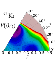
(a) ⁷²Kr

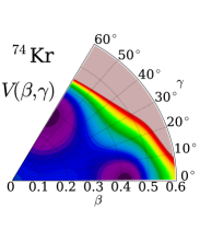
(b) ⁷⁴Kr

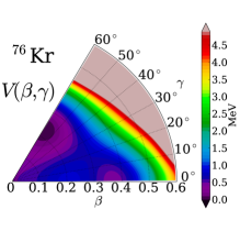
(c) ⁷⁶Kr

Figure 1: Collective potential energy surfaces $V(\beta,\gamma)$ for ^72,74,76Kr. The regions higher than 5 MeV (measured from the HFB minima) are colored rosy-brown.

In this section, we present the result of the numerical calculation for ⁷²Kr, ⁷⁴Kr, and ⁷⁶Kr and discuss properties of low-lying collective modes of excitation in these nuclei. Figure 1 shows the collective potential calculated for ^72-76Kr. All of the potential have two local minima: one is oblate and the other is prolate. The spherical shape is a local maximum in any case. In ⁷²Kr, the absolute minimum is oblate and the prolate minimum is approximately 600 keV higher. In contrast, the prolate minimum is lower than the oblate one in ⁷⁴Kr, which suggest there may occur a shape transition from oblate to prolate between these isotopes. The experimental data [6] of the spectroscopic quadrupole moments for ⁷⁴Kr and ⁷⁶Kr indicate that they are prolate in the ground band. One may expect that the absolute minimum is oblate in ⁷²Kr and it becomes prolate for $A\geq 74$. However, it is not as simple as one might expect: the oblate minimum becomes the absolute minimum again in ⁷⁶Kr. This does not necessarily mean that our calculation fails in the reproduction of the ground band shape in ⁷⁶Kr. As we shall discuss below, we have to take into account dynamical effects beyond the mean field.

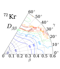
(a) $D_{\beta\beta}(\beta,\gamma)$

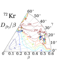
(b) $D_{\beta\gamma}(\beta,\gamma)/\beta$

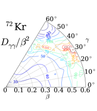
(c) $D_{\gamma\gamma}(\beta,\gamma)/\beta^{2}$

Figure 2: Vibrational inertial masses, $D_{\beta\beta}(\beta,\gamma)$, $D_{\beta\gamma}(\beta,\gamma)/\beta$ and $D_{\gamma\gamma}(\beta,\gamma)/\beta^{2}$, in unit of MeV^-1 calculated for ⁷²Kr.

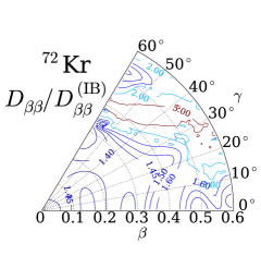
(a) $D_{\beta\beta}/D_{\beta\beta}^{\rm(IB)}$

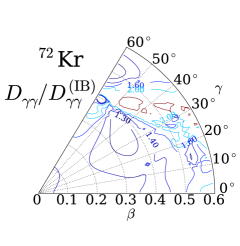
(b) $D_{\gamma\gamma}/D_{\gamma\gamma}^{\rm(IB)}$

Figure 3: Ratios of the LQRPA vibrational masses to the IB cranking masses, $D_{\beta\beta}/D^{({\rm IB})}_{\beta\beta}$ and $D_{\gamma\gamma}/D^{({\rm IB})}_{\gamma\gamma}$, calculated for ⁷²Kr.

We show in Fig. 2 the $\beta-\gamma$ dependence of the vibrational masses for ⁷²Kr. One can see their deviation from a constant. Although they have a complicated structure at large deformation compared to that at small deformation, this region hardly contributes to the calculated results as the potential is high. We also depict the ratios of the LQRPA vibrational masses to the IB vibrational masses in Fig. 3.

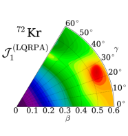
(a) ${\cal J}_{1}(\beta,\gamma)$

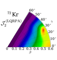
(b) ${\cal J}_{2}(\beta,\gamma)$

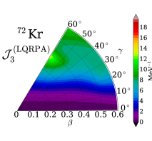
(c) ${\cal J}_{3}(\beta,\gamma)$

Figure 4: LQRPA rotational moments of inertia in unit of MeV^-1, calculated for ⁷²Kr.

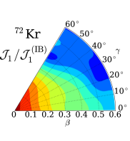
(a) ${\cal J}_{1}/{\cal J}_{1}^{\rm(IB)}$

(b) ${\cal J}_{2}/{\cal J}_{2}^{\rm(IB)}$

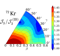
(c) ${\cal J}_{3}/{\cal J}_{3}^{\rm(IB)}$

Figure 5: Ratios of the LQRPA rotational moments of inertia to the IB cranking moments of inertia, calculated for ⁷²Kr.

We plot the LQRPA moments of inertia for ⁷²Kr in Fig. 4. We can see deviation from the irrotational moments of inertia. The ratios of the LQRPA moments of inertia to the Inglis-Belyaev ones are plotted in Fig. 5. All the ratios shown in Figs. 3 and  5 are larger than 1 on the entire ($\beta,\gamma$) plane and depends on $\beta$ and $\gamma$. This indicates not only that the time-odd components of the mean field (which enhance the inertial masses) should be taken into account but also that a simple remedy used in Refs. [31, 32, 33], i. e., a simple multiplication of a constant factor to the IB cranking moments of inertia, is insufficient.

3.1 ⁷²Kr

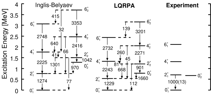
Figure 6: Excitation spectra and $B(E2)$ values calculated for ⁷²Kr by means of the CHB+LQRPA method (denoted LQRPA) and experimental data [4, 7, 8]. For comparison, results calculated using the IB cranking masses (denoted Inglis-Belyaev) are also shown. Only $B(E2)$’s larger than 1 Weisskopf unit are shown in units of $e^{2}{\rm fm}^{4}$.

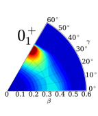
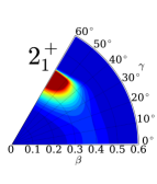
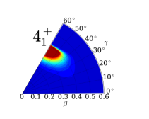
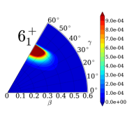
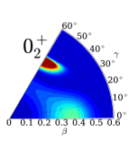
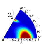
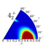
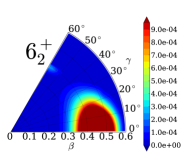
Figure 7: Vibrational wave functions squared, $\beta^{4}|\Phi_{\alpha I}(\beta,\gamma)|^{2}$, for ⁷²Kr.

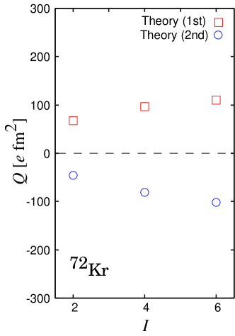
(a) ⁷²Kr

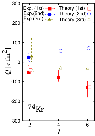
(b) ⁷⁴Kr

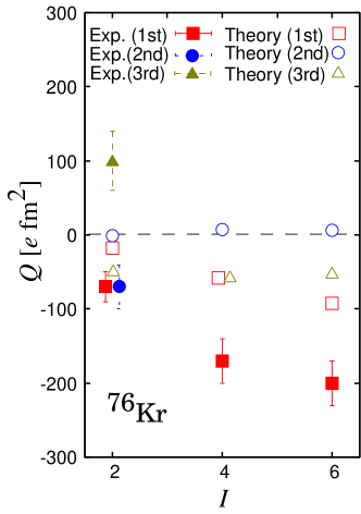
(c) ⁷⁶Kr

Figure 13: Spectroscopic quadrupole moments in unit of $e~{}{\rm fm}^{2}$ of the first (square), second (circle) and third (triangle) states for each angular momentum in ^72,74,76Kr. Calculated values are shown by open symbols, while experimental data [6] are indicated by filled symbols.

We show the excitation spectra and $B(E2)$ values calculated for ⁷²Kr in Fig. 6 together with the experimental data. The result of calculation for spectroscopic quadrupole moments are shown in Fig. 13 together with those for ^74,76Kr. In Fig. 7 the collective wave function squared, $\beta^{4}\sum_{K}|\Phi_{\alpha IK}(\beta,\gamma)|^{2}$, are plotted with a factor $\beta^{4}$ multiplied. The $\beta^{4}$ factor carries the dominant $\beta$ dependence of the volume element $G^{1/2}(\beta,\gamma)$. Note that, if the whole volume element was multiplied, all the state would look triaxial because of the factor $\sin 3\gamma$, which vanishes on the oblate and prolate lines. In Fig. 6, the result obtained using the IB cranking masses instead of the LQRPA collective masses are also shown for comparison.

As expected from Figs. 3 and 5, the excitation energies obtained with the IB cranking masses are higher than those obtained with the LQRPA collective masses. Moreover, the excitation energies obtained with the LQRPA collective masses are in better agreement with the experimental data except for the $2_{1}^{+}$ state. The observed excitation energy of the $0_{2}^{+}$ state locates close to the $2_{1}^{+}$ state. It is seen that the $0_{2}^{+}$ energy obtained with the LQRPA masses is in much better agreement with the experimental data than that with the IB cranking masses.

The collective wave function of the ground state has a peak around the oblate potential minimum. It has a tail to the prolate region, however. As angular momentum increases, the localization of the collective wave function develops. The collective wave function of the $0_{2}^{+}$ state consists of two component: one is a sharp peak on the oblate side and the other is a component spreading around the prolate region somewhat broadly. It has a node in the $\beta$ direction on the oblate side but the $\gamma$-vibrational component is strongly mixed. In contrast to the $0_{2}^{+}$ state, the effects of the $\beta$ vibrational excitation are weak for the other yrare states. The vibrational wave function has two peaks at $I=2$. The oblate peak shrinks rapidly but the prolate one grows with angular momentum due to the orthogonality to the yrast states. These behaviors of the vibrational wave function are consistent with the results of the (1+3) dimensional ASCC calculation [18, 19]. There, it is suggested that the rotational effect may assist the localization of the collective wave function.

The $E2$ transition strengths clearly indicate that the shape-coexistence-like character becomes stronger with increasing angular momentum: the interband transitions between the initial and final states having equal angular momentum become weaker and weaker.

The signs of the spectroscopic quadrupole moments shown in Fig. 13(a) are positive for the yrast states indicating their oblate-like character, while they are negative for the yrare states indicating their prolate-like character. Their magnitudes increase as angular momentum increases, which reflects the growth of localization of the vibrational wave function.

3.2 ⁷⁴Kr

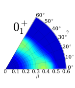
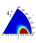
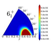
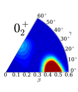
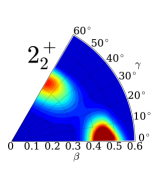
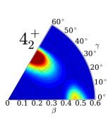
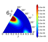
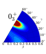
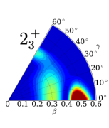
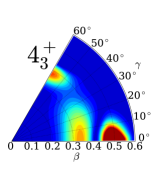
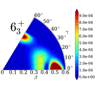
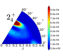
Figure 9: Vibrational wave functions squared, $\beta^{4}|\Phi_{\alpha I}(\beta,\gamma)|^{2}$, for ⁷⁴Kr.

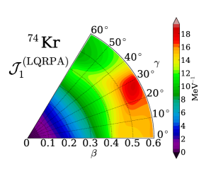
Figure 10: The LQRPA moment of inertia ${\cal J}_{1}$ for rotation about the $x$-axis, calculated for ⁷⁴Kr.

The excitation spectrum and $B(E2)$ values calculated for ⁷⁴Kr are presented in Fig. 8 together with the experimental data, while the collective wave function squared are displayed in Fig. 9. It is seen that the collective wave function of the ground state spreads over the entire $\gamma$ region along the potential valley. However, it localizes more and more on the prolate side with increasing angular momentum. This behavior results from the $\beta$-$\gamma$ dependence of the rotational moments of inertia: one can clearly see the oblate-prolate asymmetry for $\beta\gtrsim 0.4$ in the moment of inertia ${\cal J}_{1}$ displayed in Fig. 10. Although the $0_{2}^{+}$ state has somewhat a $\beta$-vibrational component, the yrare collective wave function for $I\geq 2$ has almost one-dimensional structure in the $\gamma$ direction with a constant $\beta$. While the collective wave function has a two-peak structure, the prolate peak shrinks with increasing angular momentum due to the orthogonality to the yrast state.

The third and fourth states for each angular momentum can be regarded as admixtures of $\beta$-vibrational and $\gamma$-vibrational components. On one hand, the $0_{3}^{+}$ and $2_{4}^{+}$ states have a node in the $\beta$ direction on the oblate side. On the other hand, $0_{4}^{+}$, $2_{3}^{+}$, $4_{3}^{+}$ and $6_{3}^{+}$ have a node on the prolate side.

It is clearly seen in Fig. 8 that the result of calculation reproduces well the significant enhancement of $B(E2;0_{2}^{+}\rightarrow 2_{1}^{+})$, $B(E2;2_{2}^{+}\rightarrow 0_{2}^{+})$ and $B(E2;2_{2}^{+}\rightarrow 2_{1}^{+})$, found in experiments, as well as the large $B(E2)$ values within the ground band.

The spectroscopic quadrupole moments for ⁷⁴Kr, shown in Fig. 13(b), are also in excellent agreement with the experimental data, aside from a minor disagreement for the $2_{3}^{+}$ state. In particular, the characteristic features, such as their signs and the increasing tendency of their magnitudes with angular momentum in the ground band, are well reproduced.

3.3 ⁷⁶Kr

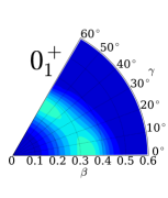
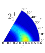
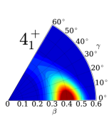
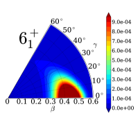
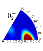
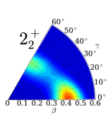
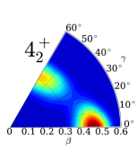
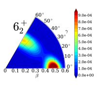
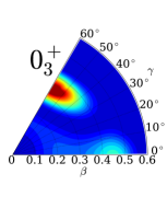
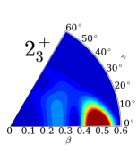
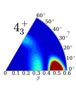
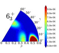
Figure 12: Vibrational wave functions squared, $\beta^{4}|\Phi_{\alpha I}(\beta,\gamma)|^{2}$, for ⁷⁶Kr.

The excitation spectrum and $B(E2)$ values calculated for ⁷⁶Kr are presented in Fig. 11 together with the experimental data, while the collective wave function squared are displayed in Fig. 12. The behavior of the collective wave function for ⁷⁶Kr is qualitatively similar to that for ⁷⁴Kr, except that the development of the localization of the yrare wave function is weaker and it has a more remarkable two-peak structure. The mechanism of appearance of the two-peak structure is discussed from a general viewpoint of oblate-prolate symmetry breaking in Ref. [41].

The difference to be most noted between ⁷⁴Kr and ⁷⁶Kr is the location of the minimum of the collective potential. One can see the importance of the rotational effect from Fig. 12. Although the potential has the oblate absolute minimum in ⁷⁶Kr, the vibrational wave functions of the $2_{1}^{+}$, $4_{1}^{+}$ and $6_{1}^{+}$ states still localize on the prolate side. It implies that the potential and rotational effects compete and the rotational effect dominates over the potential one with increasing angular momentum. This calculation serves as a good example suggesting that the nuclear shape cannot be determined only by the location of the potential minimum.

The spectroscopic quadrupole moments, shown in Fig. 13(c), qualitatively agree with the experimental data. The sign and increase with angular momentum are well reproduced for the ground band. Their absolute magnitudes are, however, too small compared with the experimental data. This seems to indicate that the calculated magnitudes of the quadrupole deformation and/or the localization of the collective wave functions in the $(\beta,\gamma)$ space are insufficient. It is interesting to note that the calculated quadrupole moment for the $2_{3}^{+}$ state better agrees with the experimental data for the $2_{2}^{+}$ state. In this connection, we notice that the $E2$ transition properties of the observed $2_{2}^{+}$ state in ⁷⁶Kr are different from those in ⁷⁴Kr: while it decays to the $2_{1}^{+}$ and $0_{2}^{+}$ states with almost equal $E2$ strengths in ⁷⁴Kr, it decays almost totally to the $0_{2}^{+}$ state in ⁷⁶Kr. This point was emphasized by Clément et al. [6]. This difference is qualitatively reproduced in our calculation if we assume that, in ⁷⁶Kr, the band consisting of the experimental $0_{2}^{+},2_{2}^{+},4_{2}^{+}$ and $6_{2}^{+}$ states corresponds to the band comprised of the calculated $0_{2}^{+},2_{3}^{+},4_{3}^{+}$ and $6_{3}^{+}$ states.

3.4 Discussion

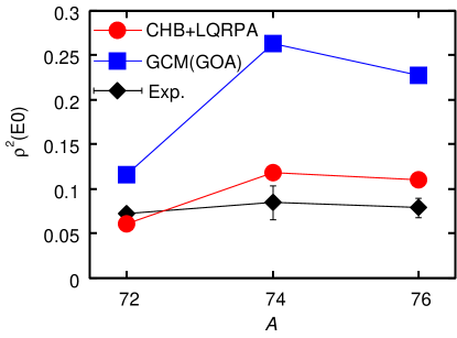
Figure 14: Electric monopole transition matrix element $\rho^{2}(E0)$ calculated using Eq. (39) in comparison with the experimental data [3, 4] and the result of the HFB-based GCM (GOA) calculation [17].

In addition to the $E2$ transition properties and the quadrupole moments of the low-lying states, we have also calculated $E0$ transition strengths $\rho^{2}(E0)$. The result of calculation is compared with the experimental data in Fig. 14. We see that the calculated result well reproduces the experimental data both qualitatively and quantitatively. The $\rho^{2}(E0)$ takes a maximal value at $A=74$, which reflects the shape transition. These $E0$ transition strengths are evaluated using Eq. (39) where the phenomenological Bohr relation [23, 39] between the $E0$ matrix elements and the quadrupole deformation is assumed. In this sense, this way of calculating $\rho(E0)$ is semi-microscopic, in contrast to the calculation of $B(E2)$ and spectroscopic quadrupole moments which are carried out in a fully microscopic way using the expectation values of the quadrupole operators at each point on the ($\beta,\gamma$) deformation space, as explained in Section 2.3. For a fully microscopic calculation of $\rho(E0)$ without assuming Bohr’s relation, we need to use a more realistic effective interaction than Baranger-Kumar’s version of the P+Q force model [36]. This task is left for future works. Note that $\rho(E0)$ vanishes in Baranger-Kumar’s P+Q force model, because this force is designed such that the radial matrix elements of the monopole operators take the same value for all single-particle states.

Let us add a few remarks concerning the results of calculation for $E2$ transition properties shown in Figs. 8 and 11. Although we have succeeded in reproducing a number of features observed in experiments, some aspects in experimental data remains unexplained. In particular, the large value of $B(E2;0_{3}^{+}\rightarrow 2_{1}^{+})$ in ⁷⁴Kr is not reproduced in the calculation. In this connection, it should be emphasized that the properties of the excited $0^{+}$ states are quite sensitive to the mixing of the $\beta$ vibrations and the large-amplitude $\gamma$ vibrations (large-amplitude fluctuations in the triaxial shape degree of freedom). In this study, we have not adjusted the interaction parameters by fitting the theoretical result to the experiment, and the interaction we have employed itself is rather simple. Therefore, it remains for future to examine whether or not these disagreements with experiments are improved when a better interaction is used.

As we mentioned in Introduction, the low-lying states of light Kr isotopes have recently been studied also by Girod et al. [17] by means of the CHFB-based GCM (GOA) method. Consistent with our results, their calculation also demonstrates that the large-amplitude fluctuation in the triaxial shape degree of freedom plays an important role in the description of the shape coexistence and the shape transition in the light Kr isotopes. They have used the Gogny D1S force, which is more realistic than the P+Q force. However, their inertial masses are derived with the cranking formula, which ignores the contribution from the time-odd mean field. We would like to emphasize that there is no problem to use a more realistic interaction within the framework of the CHFB+LQRPA method, although numerical calculation becomes much more demanding. The reason why we have used the schematic P+Q interaction in this paper is simply because this is the first application of the CHFB+LQRPA method to real nuclear collective phenomena. We shall employ a more realistic interaction like Skyrme interactions in future works. It will also become possible to use the CHFB+LQRPA method in conjunction with modern nuclear energy density functionals.

4 Conclusion

We have studied the oblate-prolate shape coexistence/mixing in the low-lying states of ^72,74,76Kr using the 5D quadrupole Hamiltonian determined microscopically by means of the CHFB+LQRPA method, which is based on the 2D ASCC method. Our results indicates a shape transition from oblate in the ground state of ⁷²Kr to prolate in ^74,76Kr, which is consistent with the experimental data. We have shown that the basic features of the low-lying spectra in these nuclei are determined by the interplay of the large-amplitude vibrations in the triaxial shape degree of freedom, the $\beta$-vibrational excitations and the rotational motions. We have furthermore shown that the rotational motion plays an important role for the growth of localization of the vibrational wave functions in the ($\beta,\gamma$) deformation space.

The authors thank T. Nakatsukasa, M. Matsuo, and K. Matsuyanagi for discussions. K. S. and N. H. are supported by the Junior Research Associate Program and Special postdoctoral Researcher Program of RIKEN, respectively. The numerical calculations were carried out on Altix3700 BX2 at Yukawa Institute for Theoretical Physics in Kyoto University and RIKEN Cluster of Clusters (RICC) facility. This work is supported by the Core-to-Core Program of the Japan Society for the Promotion of Science ”International Research Network for Exotic Femto Systems”.

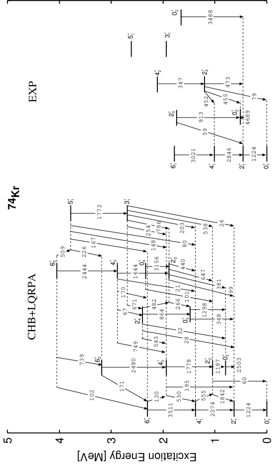
Figure 8: Same as Fig. 6 but for ⁷⁴Kr. Experimental data are taken from Ref. [6] .

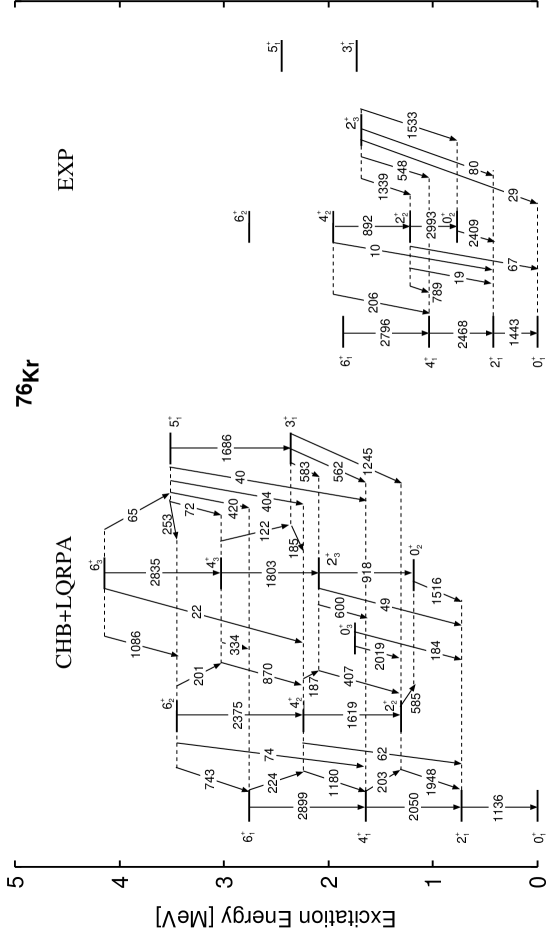
Figure 11: Same as Fig. 6 but for ⁷⁶Kr. Experimental data are taken from Ref. [6] .

References

- Piercey et al [1981] R. B. Piercey et al, Phys. Rev. Lett. 47 (1981) 1514.
- Varley et al [1987] B. J. Varley et al, Phys. Lett. B 194 (1987) 463.
- Chandler et al. [1997] C. Chandler et al., Phys. Rev. C 56 (1997) 2924.
- Bouchez et al. [2003] E. Bouchez et al., Phys. Rev. Lett. 90 (2003) 082502.
- Poirier et al. [2004] E. Poirier et al., Phys. Rev. C 69 (2004) 034307.
- Clément et al. [2007] E. Clément et al., Phys. Rev. C 75 (2007) 054313.
- Gade et al [2005] A. Gade et al, Phys. Rev. Lett. 95 (2005) 022502; Phys. Rev. Lett. 96 (2006) 189901, Erratum.
- Fischer et al. [2003] S. M. Fischer et al., Phys. Rev. C 67 (2003) 064318.
- Giannatiempo et al. [1995] A. Giannatiempo et al., Phys. Rev. C (1995) 2444.
- Nazarewicz et al. [1985] W. Nazarewicz, J. Dudek, R. Bengtsson, T. Bengtsson, I. Ragnarsson, Nucl. Phys. A 435 (1985) 397.
- Langanke et al. [2003] K. Langanke, D. J. Dean, W. Nazarewicz, Nucl. Phys. A 728 (2003) 109.
- Petrovici et al. [2000] A. Petrovici, K. W. Schmid, A. Faessler, Nucl. Phys. A 665 (2000) 333.
- Bonche et al. [1985] P. Bonche, H. Flocard, P.-H. Heenen, S. J. Krieger, M. S. Weiss, Nucl. Phys. A 443 (1985) 39.
- Yamagami et al. [2001] M. Yamagami, K. Matsuyanagi, M. Matsuo, Nucl. Phys. A 693 (2001) 579.
- Bender et al. [2006] M. Bender, P. Bonche, P.-H. Heenen, Phys. Rev. C 74 (2006) 024312.
- Próchniak [2009] L. Próchniak, Int. J. Mod. Phys. E 18 (2009) 1044.
- Girod et al. [2009] M. Girod, J.-P. Delaroche, A. Görgen, A. Obertelli, Phys. Lett. B 676 (2009) 39.
- Hinohara et al. [2008] N. Hinohara, T. Nakatsukasa, M. Matsuo, K. Matsuyanagi, Prog. Theor. Phys. 119 (2008) 59.
- Hinohara et al. [2009] N. Hinohara, T. Nakatsukasa, M. Matsuo, K. Matsuyanagi, Phys. Rev. C 80 (2009) 014305.
- Matsuo et al. [2000] M. Matsuo, T. Nakatsukasa, K. Matsuyanagi, Prog. Theor. Phys. 103 (2000) 959.
- Hinohara et al. [2007] N. Hinohara, T. Nakatsukasa, M. Matsuo, K. Matsuyanagi, Prog. Theor. Phys. 117 (2007) 451.
- Hinohara et al. [2010] N. Hinohara, K. Sato, T. Nakatsukasa, M. Matsuo, K. Matsuyanagi, arXiv:1004.5544 (2010).
- Bohr and Mottelson [1975] A. Bohr, B. R. Mottelson, Nulcear Structure, vol. II, W-A. Benjamin Inc., 1975.
- Belyaev [1965] S. T. Belyaev, Nucl. Phys. 64 (1965) 17.
- Kumar and Baranger [1967] K. Kumar, M. Baranger, Nucl. Phys. A 92 (1967) 608.
- Próchniak and Rohoziński [2009] L. Próchniak, S. G. Rohoziński, J. Phys. G: Nucl. Part. Phys. 36 (2009) 123101.
- Inglis [1954] D. R. Inglis, Phys. Rev. 96 (1954) 1059.
- Beliaev [1961] S. Beliaev, Nucl. Phys. 24 (1961) 322.
- Baranger and Vénéroni [1978] M. Baranger, M. Vénéroni, Ann. Phys. 114 (1978) 123–200.
- Dobaczewski and Skalski [1981] J. Dobaczewski, J. Skalski, Nucl. Phys. A 369 (1981) 123.
- Nikšić et al. [2009] T. Nikšić, Z. P. Li, D. Vretenar, L. Próchniak, J. Meng, P. Ring, Phys. Rev. C 79 (2009) 034303.
- Li et al. [2009] Z. P. Li, T. Nikšić, D. Vretenar, J. Meng, G. A. Lalazissis, P. Ring, Phys. Rev. C 79 (2009) 054301.
- Li et al. [2010] Z. P. Li, T. Nikšić, D. Vretenar, J. Meng, Phys. Rev. C 81 (2010) 034316.
- Delaroche et al. [2010] J.-P. Delaroche, M. Girod, J. Libert, H. Goutte, S. Hilaire, S. Péru, N. Pillet, G. F. Bertsch, Phys. Rev. C 81 (2010) 014303.
- Bes and Sorensen [1969] D. R. Bes, R. A. Sorensen, Advances in Nuclear Physics, vol. 2, Prenum Press, 1969.
- Baranger and Kumar [1968] M. Baranger, K. Kumar, Nucl. Phys. A 110 (1968) 490.
- Hinohara et al. [2006] N. Hinohara, T. Nakatsukasa, M. Matsuo, K. Matsuyanagi, Prog. Theor. Phys. 115 (2006) 567.
- Thouless and Valatin [1962] D. J. Thouless, J. G. Valatin, Nucl. Phys. 31 (1962) 211.
- Kumar [1975] K. Kumar, in: W. Hamilton (Ed.), The Electromagnetic Interaction in Nuclear Spectroscopy, North-Holland, Amsterdam, 1975.
- Sakamoto and Kishimoto [1990] H. Sakamoto, T. Kishimoto, Phys. Lett. B 245 (1990) 321.
- Sato et al. [2010] K. Sato, N. Hinohara, T. Nakatsukasa, M. Matsuo, K. Matsuyanagi, Prog. Theor. Phys. 123 (2010) 129.