High frequency polarization switching of a thin ferroelectric film

Abstract

We consider both experimentally and analytically the transient oscillatory process that arises when a rapid change in voltage is applied to a $Ba_{x}Sr_{1-x}TiO_{3}$ ferroelectric thin film deposited on an $Mg0$ substrate. High frequency ($\approx 10^{8}rad/s$) polarization oscillations are observed in the ferroelectric sample. These can be understood using a simple field-polarization model. In particular we obtain analytic expressions for the oscillation frequency and the decay time of the polarization fluctuation in terms of the material parameters. These estimations agree well with the experimental results.

I Introduction

Unique intrinsic properties make ferroelectric materials attractive both for fundamental research and applications in devices using electro-optical, piezoelectric and other effects. Bulk ferroelectric materials, particularly those based on barium-strontium titanate $Ba_{x}Sr_{1-x}TiO_{3}$ (BST) compounds Smolensky ; Vendik are attractive for high-power applications because of their high dielectric permittivity and small losses. Ferroelectric-based devices include ultra-fast electrically-controlled phase shifters for amplitude and phase control. It has been shown that the dielectric permittivity of a ferroelectric can be altered by applying an electric field. Therefore a fast ferroelectric phase shifter controlled by an electric field bias is being investigated ferro_switch to be used for applications in particle accelerators. Ferroelectric materials provide significant benefits for several applications such as switching and control elements. These are able to handle high peak and average power while maintaining a very short response time of less than just few nanoseconds. According to some estimations Smolensky , ferro_switch the response time to an applied external electric field is about  $10^{-11}$ s for crystalline and  $10^{-10}$ s for ceramic compounds. The high permittivity (over 1000) of ferroelectrics makes them potential candidates to replace silicon oxide dielectrics as storage capacitors for memory devices. A solid solution barium-strontium titanate $Ba_{x}Sr_{1-x}TiO_{3}$ (BST) has a high permittivity and a composition dependent Curie temperature $T_{c}$ which varies in a range of 30 - 400 K. This strong dependence of the dielectric constant on electric field offers the opportunity to use ferroelectrics as tunable devices. Ferroelectric based phase shifters organised in an array have the advantage of being cheap and consuming a reduced power while continuously tuning the phase of a high power microwave signal. This rapid electrical steering is realized by adjusting the bias voltages on each element. See for example Vendik_ph_shift_ferroel and Romanofsky where the phase shifting elements based on BST thin film capacitors are discussed. There is a certain advantage in using elements build on thin ferroelectric films because of their compactness and parameter tunability. The presence of internal stresses in the thin film ferroelectrics changes their electromechanical and dielectric properties drastically. Because of this the dielectric permittivity in a thin film is reduced by about an order of magnitude compared to one for the bulk media. However choosing the appropriate substrate allows to adjust the internal stress level and tune the physical properties of the thin ferroelectric films. Thin films of BST deposited by the sputtering technique are discussed in capacitors , gatech_capacitors in reference to the production of compact tunable capacitors. These elements are attractive for applications in adaptive impedance matching networks and tunable filters. Size effects in thin ferroelectric films are discussed in Fridkin2 . It is reported that no critical film thickness is required to obtain polarization switching.

A noteworthy transient effect occurs in ferroelectric material subjected to an alternating electric field which causes polarization switching between two stationary states of the ferroelectric. The switching process is followed by high-frequency polarization oscillations around their stationary states. Basically the polarization dynamics of a ferroelectric near its steady state can be viewed in terms of a damped oscillator with an eigenfrequency determined by the material parameters. An alternating electric field serves as the external force that pushes the oscillator away from its equilibrium. The generation of infrared (IR) radiation by means of polarization switching was proposed for ferroelectrics Balkarei . There the authors estimate the energy radiated using the dipole approximation.

The study of the transient dynamics of these processes can help understand how the system parameters can be adjusted to provide the required transient behavior. That is important for devices subjected to sharp/shock periodic or aperiodic forces of high frequency. They then spend most of their time in a transient state, even if the relaxation time is smaller than the observation period. Transient processes occurring in ferroelectric might become unwanted effects if the possible applications require fast switching between polarization states, such as in FeRAM. In opposite they might be required if the polarization switching is used to produce oscillations that will form an IR pulse. The polarization relaxation time and oscillation frequency are important characteristics of this transient behavior. The polarization damping constant in ferroelectrics is of the order of $10^{10}s^{-1}$, as indicated in Fridkin . The theoretical description for an isotropic paraelectric in the framework of the dynamical Landau-Khalatnikov model being investigated in Osman_Ishib_Tilley1 ; Osman_Ishib_Tilley2 allows to calculate nonlinear susceptibility coefficients.

Here we discuss an experiment where we observe the polarization dynamics in a thin BST film. A similar experiment studying fast polarization switching was performed earlier by some of the authors. The method of observation of the polarization uses the second harmonic generation in the thin film of the BST solid solution. It is discussed in Mishina_apl . In the present experiment we follow a pump-probe procedure. First we apply a constant field $E_{s}$ and obtain the steady state induced polarization $P_{s}$. Then we send in an additional small electric field pulse to probe the film. In principle this time dependent solution could be described by the theory set up in cmk but we chose in this first study to describe the relaxation response of the film. For that we set up a scattering theory formalism. The bound states of the system $(E,P)$ will then give the response of the film, ie the typical oscillation frequency and the radiative decay time. We identify two channels of damping, the radiative damping and the inner damping. From the experimental data we estimate the magnitude of both terms and find that here the inner damping dominates. There could be other experiments where the contrary happens ie the radiative damping may dominate.

II Model of electromagnetic response in ferroelectric film

The theory of ferroelectric has started to develop in the 1930s. The phase transition theory proposed by Landau Landau_JETP , Landau_stat1 was applied to describe the behavior of the ferroelectric near a critical point of the phase transition. Following the Landau-Ginzburg-Devonshire theory the thermodynamic Gibbs potential $\Phi$ in the neighborhood of the critical point can be represented as a power series of the order parameter, namely the polarization Ginzburg45 , Ginzburg49 , Ginzburgufn up to 4-th order, and Devonshire up to terms of order $P^{6}$.

$$\Phi=\Phi_{0}+\frac{\alpha}{2}P^{2}+\frac{\beta}{4}P^{4}-EP.$$

The expansion coefficients are $\alpha=a_{0}(T-T_{c})$ and $\beta$. $T_{c}$ is the Curie temperature. In a solid solution $Ba_{x}Sr_{1-x}TiO_{3}$ the Curie temperature depends on the relative concentration $x$ of barium. The approximate formula to calculate $T_{c}$ in BST was proposed by Lemanov . It reads $T_{c}=360x+40$. Particularly $T_{c}=292K$ for $x=0.7$. This is the concentration of barium in the thin film investigated in an experiment on ferroelectric switching Mishina_apl .

We describe an experiment where a thin film of thickness $l$ is deposited on a dispersionless substrate. The optical properties of the surrounding media can be characterized by the refractive index $n(z)$, such that $n(z)=1$ for $z<0$ and $n(z)=n>1$ for $z>0$, i.e. in the substrate. The electric field $E(z,t)$ is governed by the Maxwell equation and the polarization obeys the equation of a damped oscillator driven by the field (compare to cmk )

$${\partial^{2}E\over\partial z^{2}}-{n^{2}\over c^{2}}{\partial^{2}E\over\partial t^{2}}=\frac{l}{\epsilon_{0}c^{2}}{\partial^{2}P\over\partial t^{2}}\delta\left(z\right),$$

(1)

$$\frac{\tau^{2}}{\epsilon_{0}}\frac{\partial^{2}P}{\partial t^{2}}+\frac{\gamma\tau^{2}}{\epsilon_{0}}\frac{\partial P}{\partial t}+\alpha P+\beta P^{3}=E_{f}(t),$$

where $E_{f}(t)$ is the electric field inside the thin film. The constant $\tau$ is proportional to the inverse of the Born frequency, this value will be estimated for BST later. Typically the decay constant $1/(\gamma\tau^{2})$ is small Ginzburgufn . However we take it into account for generality.

The electromagnetic wave is incident from the left of a film located at $z=0$. Thus the electric fields outside the thin film $E^{-}(z,t)$ for $z<0$ and $E^{+}(z,t)$ for $z>0$ are defined by free wave equations. The time Fourier images of these fields can be written as

$$\tilde{E}^{-}(z,\omega)=Ae^{ik_{1}z}+Be^{-ik_{1}z},$$

$$\tilde{E}^{+}(z,\omega)=Ce^{ik_{2}z}.$$

Here $k_{1}=\omega/c$ and $k_{2}=\omega n/c$ are the wave numbers on the left and on the right of the thin film, $A$ is the Fourier amplitude of the incident wave, $B$ is the Fourier amplitude of the reflected wave and $C$ is the Fourier amplitude of the transmitted wave.

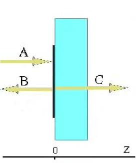
Figure 1: Schematics of the experimental setup where an electric field pulse polarizes a ferroelectric thin film deposited on a substrate.

According to the boundary conditions at $z=0$ cmk ; Rupasov the electric field $\tilde{E}$ and its spatial derivative $\tilde{E_{,z}}$ are connected by the relations

$$\tilde{E}^{(-)}(z=0,\omega)=E^{(+)}(z=0,\omega),$$

$$\tilde{E}_{,z}^{(-)}(z=0,\omega)-E_{,z}^{(+)}(z=0,\omega)=\frac{l\omega^{2}}{c^{2}\epsilon_{0}}P(\omega),$$

where $P(\omega)$ is the Fourier image of the thin film polarization. This leads to the following equations for the Fourier amplitudes of the left and right electric fields

$$A+B=C,\hskip 10.00002ptA-B=nC-\frac{il\omega}{c\epsilon_{0}}P(\omega).$$

Hence the amplitude of the transmitted wave $C$ and the amplitude of the reflected wave $B$ can be expressed through the amplitude $A$ of the incident wave and the thin film polarization $P(\omega)$:

$$C=\frac{2}{n+1}A+\frac{il\omega}{c(n+1)\epsilon_{0}}P(\omega),$$ (2)

$$B=\frac{1-n}{1+n}A+\frac{il\omega}{c(n+1)\epsilon_{0}}P(\omega).$$ (3)

Using the inverse Fourier transform we obtain the amplitude of the electric field inside the thin film $E_{f}$ as $E^{+}(z,t)$ at $z=0$ Rupasov , i.e.,

$$E_{f}(t)=\frac{2}{1+n}E_{in}(t)-\frac{l}{c(n+1)\epsilon_{0}}\frac{\partial P}{\partial t},$$

where $E_{in}(t)$ is the electric field of the incident wave. Thus one can find from the second equation of the system (1) that the polarization of the ferroelectric thin film is governed by the following equation

$$\frac{\tau^{2}}{\epsilon_{0}}\frac{\partial^{2}P}{\partial^{2}t}+\left(\frac{\gamma\tau^{2}}{\epsilon_{0}}+\frac{l}{c(n+1)\epsilon_{0}}\right)\frac{\partial P}{\partial t}+$$

$$\qquad~{}~{}~{}~{}+\alpha P+\beta P^{3}=\frac{2}{1+n}E_{in}(t).$$ (4)

This expression shows that two relaxation channels exist. One of them is the ordinary one related with inner friction i.e., the $\gamma$-term. The second relaxation channel is due to the radiation process. The variation of the polarization generates the electromagnetic field outside the film.

The polarization of the thin film evolves according to (4) as an oscillator with damping and a forcing that is equal to $E_{s}=2E_{in}(t)/(1+n)$. Furthermore, this equation allows to consider $E_{in}$ as a constant electric field i.e. a constant voltage. In this case $E_{s}=V_{s}/l$ where $V_{s}$ is the applied voltage.

II.1 Relaxation to a steady state polarization

In the absence of an external electric field the ferroelectric possesses two equilibrium states, each corresponding to different polarities. In the paraelectric phase there is only one equilibrium corresponding to an unpolarized state. The experiment under consideration was performed at room temperature which is above the Curie temperature for BST so that the sample is in the paraelectric state. However there is another way to change the polarization state. This can be induced by applying an external field or a stress. In this experiment we chose to do the former. The induced steady state polarization $P_{s}$ is defined as the fixed point of the equation (1) where we assume that the electric field $E_{f}(t)=E_{s}$ is constant and the polarization $P=P_{s}$ are time independent. We get

$$\alpha P_{s}+\beta P_{s}^{3}=E_{s}.$$ (5)

We assume the solution of (1) to be of the form

$$E=E_{s}+\delta E,~{}~{}~{}P=P_{s}+\delta P,$$ (6)

where $\delta E$ and $\delta P$ are small compared respectively to $E_{s}$ $P_{s}$. Plugging this into the equations (1) we get the linearized equations around the stationary solution $(E_{s},P_{s})$

$${n^{2}\over c^{2}}{\partial^{2}\delta E\over\partial t^{2}}-{\partial^{2}\delta E\over\partial z^{2}}=-\frac{l}{\epsilon_{0}c^{2}}\frac{\partial^{2}\delta P}{\partial t^{2}}\delta\left(z\right),$$

(7)

$$\frac{\tau^{2}}{\epsilon_{0}}\frac{\partial^{2}\delta P}{\partial t^{2}}+\frac{\gamma\tau^{2}}{\epsilon_{0}}\frac{\partial\delta P}{\partial t}+(\alpha+3\beta P_{s}^{2})\delta P=\delta E(t).$$

II.2 Scattering of linear waves by the thin film

We now proceed to solve the linearized equations (7) by using a scattering theory formalism. We separate time and space by assuming a periodic solution

$$\delta E=e(z)e^{-i\omega t},~{}~{}~{}\delta P=pe^{-i\omega t}.$$ (8)

We get

$$n^{2}k^{2}e+{\partial^{2}e\over\partial z^{2}}=-\frac{l}{\epsilon_{0}}k^{2}\delta\left(z\right)p,$$

(9)

$$(\Omega^{2}+i\gamma\tau^{2}\omega-\tau^{2}\omega^{2})p=\epsilon_{0}e(0),$$

where the wave number $k=\omega/c$ and where we introduced

$$\Omega^{2}=\epsilon_{0}(\alpha+3\beta P_{s}^{2}).$$ (10)

In the scattering we assume the electromagnetic wave to be incident from the left of the film located at $z=0$. We then have

$$e=e^{ikz}+Re^{-ikz}~{},z<0~{};~{}~{}~{}~{}e=Te^{iknz},z>0~{}~{},$$ (11)

where $R$ is the amplitude of the reflected wave and $T$ the amplitude of the transmitted wave. These expressions are related to the $A,~{}B,~{}C$ parameters of the previous section through the relations $R=B/A,~{}T=C/A$. We have the following interface conditions at $z=0$ cmk ; Rupasov

$$e(0^{-})=e(0^{+}),~{}~{}-[e_{z}]_{0^{-}}^{0^{+}}=k^{2}{l\over\epsilon_{0}}p.$$ (12)

They imply

$$1+R=T,~{}~{}nT-(1-R)=-ik{l\over\epsilon_{0}}p$$

Using the second relation of (9) to obtain $p$ we get the transmission coefficient $T$

$$T={2c(\Omega^{2}+i\gamma\tau^{2}\omega-\tau^{2}\omega^{2})\over c(n+1)(\Omega^{2}+i\gamma\tau^{2}\omega-\tau^{2}\omega^{2})+il\omega}.$$ (13)

The refraction coefficient is

$$R={c(1-n)(\Omega^{2}+i\gamma\tau^{2}\omega-\tau^{2}\omega^{2})-il\omega\over c(1+n)(\Omega^{2}+i\gamma\tau^{2}\omega-\tau^{2}\omega^{2})+il\omega}.$$ (14)

The bound states are the poles of the reflexion and transmission coefficients. Their existence indicates that the system has resonant modes that can be excited by an incoming wave. The real part of the bound states is the oscillation frequency and the imaginary part is the inverse of the decay time of the mode.

The poles of $R,T$ are given by

$$c(n+1)(\Omega^{2}+i\gamma\tau^{2}\omega-\tau^{2}\omega^{2})+il\omega=0,$$

which is the second degree equation

$$\omega^{2}\tau^{2}-i\omega\left({l\over(n+1)c}+\gamma\tau^{2}\right)-\Omega^{2}=0,$$ (15)

whose roots are

$$\omega={i\over 2}\left({l\over(n+1)c}+\gamma\right)\mp\sqrt{{\Omega^{2}\over\tau^{2}}-{1\over 4}\left[{l\over(n+1)c}+\gamma\right]^{2}}.$$ (16)

The imaginary part and real part of $\omega=\omega_{r}+i\omega_{i}$ give respectively the decay time $T_{dec}$ and the oscillation period $T_{osc}$

$$T_{dec}={1\over\omega_{i}},~{}~{}~{}T_{osc}={2\pi\over\omega_{r}}.$$ (17)

We will estimate these parameters for the experiment in the next section.

II.3 Green function solution of the linearized equation

The linearized equation

$$\frac{\tau^{2}}{\epsilon_{0}}\frac{\partial^{2}\delta P}{\partial t^{2}}+\frac{\tau^{2}\gamma}{\epsilon_{0}}\frac{\partial\delta P}{\partial t}+(\alpha+3\beta P_{s}^{2})\delta P=\delta E(t),$$

can be solved to obtain the polarization response $\delta P(t)$ to a give incoming electric field $\delta E(t)$. For that we introduce the Green function $G(t-t_{0})$ which satisfies

$$\tau^{2}\frac{\partial^{2}G}{\partial t^{2}}+\tau^{2}\gamma\frac{\partial G}{\partial t}+\Omega^{2}G=\epsilon_{0}\delta(t-t_{0}).$$ (18)

Using the Laplace transform

$${\hat{G}}(s)\equiv\int_{0}^{\infty}e^{-st}G(t)dt,$$

and assuming that $G(0)=0$ and $\partial G/\partial t(0)=0$ we obtain

$${\hat{G}}(s)={\epsilon_{0}e^{-st_{0}}\over\tau^{2}s^{2}+\tau^{2}\gamma s+\Omega^{2}}.$$ (19)

To get the inverse Laplace transform one expands this rational function as

$${\hat{G}}(s)={\epsilon_{0}\over 2(s_{1}-s_{2})}\left({e^{-st_{0}}\over s-s_{1}}-{e^{-st_{0}}\over s-s_{2}}\right),$$

where $s_{1}$, $s_{2}$ are the roots of the denominator of (19). This yields the Green function

$$G(t-t_{0})={\epsilon_{0}\over 2(s_{1}-s_{2})}\left[e^{s_{1}(t-t_{0})}-e^{s_{1}(t-t_{0})}\right],~{}~{}t>t_{0}$$

$$G(t-t_{0})=0,~{}~{}~{}~{}~{}~{}~{}~{}~{}~{}~{}~{}t<t_{0}$$

The roots are complex conjugate $s_{1}=\omega_{i}+i\omega_{r}$ , $s_{2}=\omega_{i}-i\omega_{r}$ so we obtain the final result

$$G(t-t_{0})=e^{\omega_{i}t}{\sin[\omega_{r}(t-t_{0})]\over 2\omega_{r}},~{}~{}t>t_{0}$$

(20)

$$G(t-t_{0})=0\qquad\qquad\qquad\qquad~{}t<t_{0}$$

The polarization response $\delta P(t)$ to a given perturbation of the electric field $\delta E(t)$ is the convolution integral

$$\delta P(t)=\int_{-\infty}^{t}G(t-t_{0})\delta E(t_{0})dt_{0}.$$ (21)

II.4 Induced polarization caused by a short electric pulse

Now let us consider an alternative method to investigate the polarization response. Suppose that a ferroelectric film is in a polarized state $P_{s}$ caused by a constant electric field $E_{s}$. At certain moment we send in a short electric pulse so the polarization of the film changes during a short time period. After that the polarization relaxes to the steady state position $P_{s}$. If the electric pulse is sufficiently short i.e. close to a ”$\delta$ function” then the polarization response will follow the Green function (20). We term this action ”$\delta$-function-like pushing”  the nonequilibrium polarization.

The linearization of the equation for the polarization (4) near the steady state $P_{s}$ assuming $P=P_{s}+p$ with the condition $p<<P_{s}$ results in the equation for the Green function (18). Let us suppose that the extremely short electric pulse acts at $t=0$. Then we can conclude that the evolution of $p(t)$ after $t=0$ is described by

$$p(t)\sim e^{\omega_{i}t}{\sin[\omega_{r}t)]\over 2\omega_{r}}.$$

Hence the polarization decay rate is defined by the imaginary part of the complex frequency (16), $\omega_{i}$ and the corresponding time for the polarization to attain the equilibrium is

$$T_{dec}=1/\omega_{i}.$$

The real part of the frequency (16) corresponds to oscillations of the polarization as it is approaches the steady state value. Here we recover the results obtained using the scattering formalism.

III Experimental results

The experiment was performed using the nonlinear optical stroboscopic technique as in Mishina_apl . For the second harmonic (SH) generation, the radiation of a titanium-sapphire laser (MaiTai, New-Port-SpectraPhysics) was used with a pulse duration of 100 fs, a wavelength of 780 nm, a repetition rate of 100 MHz and an average power of 100 W. The experiment was performed at room temperature. The $70nm$ thick $Ba_{0.7}Sr_{0.3}TiO_{3}$ films were deposited onto a $MgO$ substrate by RF sputtering. For such a composition, the Curie temperature equals $Tc=20$ C. However for thin films the phase transition is blurred around this value and this is confirmed by the presence of a narrow hysteresis above $T_{c}$ Mishina_apl . A voltage pulse of duration about $25$ ns, produced by an Avtech pulse generator, was applied to the copper contacts on the BST film. The polarization response of the ferroelectric film was measured as the coherent SH intensity experiment .

Figures 2 and 3 show the polarization response as a function of time of the BST thin film to electric pulses having the same amplitudes and opposite polarities. The left panels show the incoming electric field pulses as a function of time and the right panels show the SH intensity (proportional to the square of the polarization) as a function of time. In figure 2 the electric field pulse (left panel in the figure) is realized by a rapid spiking to a zero value from a constant negative voltage background with return to the same constant negative value. For figure 3 the electric pulse (left panel at the figure) drops from its constant positive value to zero and returns to the constant. In both measurements the spiking pulse will be called the ’zero’ pulse. The pulse profile is intended to have a narrow bell shape, however because of certain setup drawbacks a low-amplitude tail appears. In the right panels of Figures 2 and 3 it can be seen that the polarization oscillates long after the ’zero’ electric pulse has passed through the thin film. Then the eigenfrequency of the polarized thin film can be determined.

In both pictures the polarization oscillates around its stationary values (defined by the constant background electric field) with very close oscillations periods, about $60$ ns. This agrees with the relation (22) in the limit when the second term can be neglected in the square root because $\Omega$ only depends on the amplitude $|E_{s}|$.

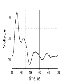
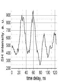
Figure 2: Plots of a ${}^{\prime}zero^{\prime}$ electric pulse as a function of time (left panel) and the subsequent polarization oscillations of the film as a function of time (right panel). The constant field $E_{s}$ is negative.

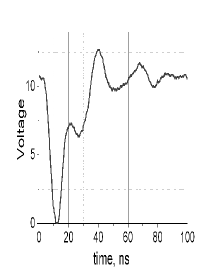
Figure 3: Plots of a ${}^{\prime}zero^{\prime}$ electric pulse and the subsequent polarization oscillations of the film as in Figure 2 except that the constant field $E_{s}$ is positive.

The next figure (4) shows the polarization dynamics when there is no constant electric field $E_{s}$ after a delta function like electric pulse of negative polarity (shown in the left panel) passes through the film. This type of electric pulse is the analog of a ’normal pulse’ studied experimentally in Mishina_apl . When the film is not polarized the SH cannot be generated, so that its intensity is about zero. The SH signal from the perturbed unpolarized state is a few times smaller than the one for the previous experiments. There the steady polarized state of the thin film was studied by a ’zero’ pulse. There are almost no polarization oscillations when perturbing a non polarized thin film. Again this agrees with the estimate (22).

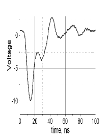
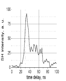
Figure 4: Left panel, plot of the electric field pulse as a function of time for a ”normal pulse” (see text). The right panel shows the subsequent polarization of the thin film as a function of time.

III.1 Discussion of the experimental results

There is a relatively broad range of experimentally obtained values of the Landau coefficients in BST solid solutions. The numbers vary with the fabrication method. The Landau coefficients found by Alpay_jap06 for a BST solid solution $Ba_{0.7}Sr_{0.3}TiO_{3}$ in SI units are presented in Table I.

$T_{c},~{}[C]$	$\alpha,[m/F]$	$\beta,[m^{5}/C^{2}F]$
34	$2.2\cdot 10^{6}$	$2.52\cdot 10^{8}$

Table 1: Material parameters for $Ba_{0.7}Sr_{0.3}TiO_{3}$ .

In the experiment performed the film thickness is $l=70nm$ (as in Mishina_apl ). We assume that the substrate refraction index is $n=1.5$. These parameters enable to calculate the frequency $\Omega$. For a normal pulse the applied voltage $V_{s}=0$ so $E_{s}=0$ and $P_{s}=0$. This gives $\Omega^{2}=\epsilon_{0}\alpha\approx 210^{-5}$. In the presence of an electric field $E_{s}=V_{s}/l$ where $V_{s}=10Volts$ we have $E_{s}\approx 10^{8}V/m$ so that from (5) we get $P_{s}\approx 0.79C/m^{2}$. This gives $\Omega^{2}=\epsilon_{0}\alpha\approx 1.810^{-3}$.

First let us estimate the term $l[(n+1)c]^{-1}$ in the formula (16). We have $l[(n+1)c]^{-1}\approx 10^{-16}$ which is very small so that this radiative damping can be completely neglected for this particular experimental situation.

	$\gamma=10^{6}[s^{-1}]$	$10^{7}$	$10^{8}$	$10^{9}$
$\tau=10^{-6}[s]$	$10^{-6}$	$10^{-7}$	$10^{-8}$	$10^{-9}$
$10^{-7}$	$10^{-6}$	$10^{-7}$	$10^{-8}$	$10^{-9}$
$10^{-8}$	$1.4\cdot 10^{-6}$	$10^{-7}$	$10^{-8}$	$10^{-9}$
$10^{-9}$	$2\cdot 10^{-6}$	$1.4\cdot 10^{-7}$	$10^{-8}$	$10^{-9}$
$10^{-10}$	$2\cdot 10^{-6}$	$2\cdot 10^{-7}$	$1.4\cdot 10^{-8}$	$10^{-9}$
$10^{-11}$	$2\cdot 10^{-6}$	$2\cdot 10^{-7}$	$2\cdot 10^{-8}$	$1.4\cdot 10^{-9}$
$10^{-12}$	$2\cdot 10^{-6}$	$2\cdot 10^{-7}$	$2\cdot 10^{-7}$	$2\cdot 10^{-9}$

Table 2: The decay time $T_{dec}$ as a function of the parameters $(\tau,\gamma)$ for the zero pulse $V_{s}=0$ volts.

¿From the experimental data it can be seen that the polarisation response for a voltage $V_{s}=0$ is qualitatively different from the one for $V_{s}=10$ volts. In particular it has a smaller decay time and practically no oscillations. Let us estimate the decay time $T_{dec}$ from (16). We have

$$T_{dec}=2/\gamma$$

if $(\Omega^{2}/\tau^{2}-\gamma^{2}/4)>0$, otherwise

$$T_{dec}=\left({\gamma\over 2}+\sqrt{{\gamma^{2}\over 4}-{\Omega^{2}\over\tau^{2}}}\right)^{-1}.$$

This decay time is shown in Table II for different values of the free parameters $(\tau,\gamma)$. Clearly if $(\Omega^{2}/\tau^{2}-\gamma^{2}/4)>0$ there will be oscillations in the polarization. Comparing the estimates of the table with the result shown in Fig. 4 indicates that $\gamma\approx 10^{7}s^{-1}$. This agrees with the value obtained in a previous study by the authors experiment .

	$\gamma=10^{6}~{}[s^{-1}]$	$10^{7}$	$10^{8}$	$10^{9}$
$\tau=10^{-6}~{}[s]$	0	0	0	0
$10^{-7}$	$1.5\cdot 10^{-5}$	0	0	0
$10^{-8}$	$9.6\cdot 10^{-7}$	$1.5\cdot 10^{-6}$	0	0
$10^{-9}$	$9.6\cdot 10^{-8}$	$9.6\cdot 10^{-8}$	$1.5\cdot 10^{-7}$	0
$10^{-10}$	$9.6\cdot 10^{-9}$	$9.6\cdot 10^{-9}$	$9.6\cdot 10^{-9}$	$1.5\cdot 10^{-8}$
$10^{-11}$	$9.6\cdot 10^{-10}$	$9.6\cdot 10^{-10}$	$9.6\cdot 10^{-10}$	$9.6\cdot 10^{-10}$
$10^{-12}$	$9.6\cdot 10^{-11}$	$9.6\cdot 10^{-11}$	$9.6\cdot 10^{-11}$	$9.6\cdot 10^{-11}$

Table 3: The oscillation period $T_{osc}$ as a function of the parameters $(\tau,\gamma)$ for the non zero pulse $V_{s}=10$ volts.

Let us now compare the oscillation period obtained for the non zero pulse $V_{s}=10$ volts with the estimate (16). We have

$$T_{osc}=2\pi\left(\sqrt{{\Omega^{2}\over\tau^{2}}-{\gamma^{2}\over 4}}\right)^{-1}.$$ (22)

This value is computed for different values of $\gamma$ and $\tau$ and reported in Table III. The zero entries correspond to the situation where $\Omega^{2}/\tau^{2}-\gamma^{2}/4<0$. As can be seen the values closest to what is observed in the experimental plots Figs. 2 and 3 are $\tau=10^{-10}s$ and $\gamma=10^{7}$. This value of the oscillation time $\tau$ agrees with the one that can be computed using the speed of sound $c_{s}=510^{3}m/s$ in the material and the film thickness $l$. We get $\tau=l/c_{s}\approx 10^{-11}s$. The estimate for the bulk material using the Newton equation describing the lattice oscillations $\tau^{2}_{hf}\approx M\epsilon_{0}/(Ne^{2})\approx 10^{-26}s^{-2}$ where $M$ is the atomic mass of BST gives $\tau\approx 10^{-13}s$ which is much too small.

We have used the expression (21) to compute the polarization response of the system to a given perturbation $\delta E$ of the electric field. We assume a gaussian $\delta E$

$$\delta E(t)=\exp\left(-{t^{2}\over 2w_{e}}\right),$$ (23)

and normalize times by $T=10ns$. We chose $\gamma=10^{7}s^{-1},~{}\tau=10^{-10}s$. In the normalized units we have $\gamma=0.1,~{}w_{e}=1$. The normalized frequency $\omega=0.45$ for the zero pulse and $\omega=4.5$ for the normal pulse. We calculated the polarization response by numerical integration using the trapeze method. To compare with the experimental data we computed $\delta P^{2}$. The results are presented in Fig. 5 for a normal pulse ($E_{s}=0$) in the left panel and for a zero pulse in the right panel. One can see on the left side of the plots the first response of the polarization. We have omitted it because it is the forced response due to the probing pulse $\delta E$. We only present the subsequent free evolution of $\delta P$. For $V_{s}=0$ the polarisation decays with few oscillations. For $V_{s}=10volts$ the polarization oscillates much longer. This is in quantitative agreement with the experimental plots presented above.

Figure 5: The polarization response of the film for a normal pulse ($E_{s}=0$) (left panel) and for a zero pulse (right panel).

IV Conclusion

We analyzed the polarization oscillations occurring in a thin ferroelectric film as a short electric pulse crosses it. We consider that the ferroelectric is in the paraelectric phase (high temperature). As in a pump probe experiment the film is initially in a static polarization state $P_{s}$ induced by a constant voltage $V_{s}$. Using the Landau-Ginzburg-Devonshire theory we computed this static polarization and the subsequent oscillations of the polarization induced by a short voltage pulse. These were analyzed using a scattering theory formalism and a Green’s function approach. Two channels of dissipation were identified, a radiative damping and an intrinsic damping.

This theory was applied to explain the experimental time evolution of the polarization for a thin ferroelectric film of BST. The polarisation is estimated indirectly through second harmonic generation. For this experimental situation we show that the radiative damping can be neglected and only the intrinsic damping should be considered. From a comparison of our model to the experimental plots we estimated the important parameters $\tau$ the response time and $\gamma$ the relaxation coefficient. Using these values our theoretical estimates of the decay time and of the oscillation period agree well with the observations. In particular for a normal pulse for which $V_{s}=0$ the damping dominates and we only see a few oscillations of the polarization. On the contrary for a zero pulse for which $V_{s}=10volts$ the damping time is longer compared with the oscillation period. Here we obtain many oscillations of the polarization.

Although the radiative damping appears as artificial in this particular high temperature situation, at low temperature phonons become frozen and the radiative damping may become predominant. The model can be further elaborated by including the spatial inhomogeneity of the thin film, the depolarization effects of the boundaries, and taking into account the internal stresses of the film. Also the dynamics of the polarization of a thin film multilayered structure can be investigated by generalizing the model.

V Acknowledgments

JGC thanks the Centre de Ressources Informatiques de Haute-Normandie for the use of its computing facilities. AIM is grateful to the Laboratoire de Mathématiques, INSA de Rouen for hospitality and support. This research was supported by RFBR grants No. 09-02-00701-a and 09-07-12144-ophi.

References

- (1) G.A. Smolensky, Ferroelectrics and Related Materials, Academic Press, New York, (1981).
- (2) O. Vendik, Ferroelectrics at Microwave. O.G.Vendik, Editor, Moscow, Radio, p.44, (1979).
- (3) A. Kanareykin, E.Nenasheva, V.Yakovlev, A.Dedyk, S.Karmanenko, A.Kozyrev, V.Osadchy, D.Kosmin, P.Schoessow, A.Semenov, arXiv:physics/0612240v1 [physics.acc-ph]
- (4) V. Sherman, K. Astafiev, N. Setter, A. Tagantsev, O. Vendik, I. Vendik, S. Hoffmann-Eifert,and R. Waser, IEEE Microwave and Wireless Components Letters, Vol. 11, No. 10, 407-409, (2001)
- (5) R. Romanofsky, J. Bernhard, G. Washington, F. VanKeuls, F. Miranda, and C. Cannedy, IEEE Trans. MTT, Vol. 48, No. 12, 2504-2510 (2000)
- (6) M. Klee et all, IEEE Transactions on Ultrasonics, Ferroelectrics, and Frequency Control, 56, 8 (2009)
- (7) Y.-K. Yoon, D. Kim, M. G. Allen, J. S. Kenney, and A. T. Hunt, IEEE Transactions on microwave theory and techniques, 51, 12 (2003)
- (8) L.M. Blinov, V.M. Fridkin, S.P. Palto, A.V. Bune, P.A. Dowben, S. Ducharme ”Two-dimensional ferroelectrics” Phys. Usp. 43 243 (2000)
- (9) Yu.I. Balkarei and E.V. Chenskii JETP Pis. Red. 13, 5, 266-269 (1971)
- (10) V. Fridkin, A. Ievlev, K. Verkhovskaya, G. Vizdrik, S. Yudin, S. Ducharme, Ferroelectrics 314, 37 (2005)
- (11) J. Osman, Y. Ishibashi and D. R. Tilley, Jpn. J. Appl. Phys. 37, 4887-4893 (1998)
- (12) R. Murgan, D.R. Tilley, Y. Ishibashi, J.F. Webb, and J. Osman, JOSA B, Vol. 19, Issue 9, 2007-2021 (2002)
- (13) J.-G. Caputo, E. V. Kazantseva, and A. I. Maimistov, Phys. Rev. B 75, 014113 (2007)
- (14) E.D. Mishina, N.E. Sherstyuk, V.I. Stadnichuk, A. S. Sigov, V. M. Mukhorotov, Yu. I. Golovko, A. van Etteger and Th. Rasing, Appl. Phys. Lett. 83, 12 2402-2404 (2003)
- (15) L.D. Landau, JETP 7, 19 62 (1937) (in Russian)
- (16) L.D. Landau, E.M. Lifshitz,”Statistical Physics” Third Edition, Part 1: Volume 5, Butterworth-Heinemann, (1980).
- (17) V.L. Ginzburg, JETP 15, 739 (1945) (in Russian)
- (18) V.L. Ginzburg, JETP 19, 36 (1949) (in Russian)
- (19) V.L. Ginzburg Phys. Usp. 44 1037 (2001)
- (20) A.F. Devonshire Philos. Mag. 40 1040 (1949)
- (21) V.V. Lemanov, Phys. Solid State 39, 318 (1997)
- (22) V.I. Rupasov and V. I. Yudson, Sov. J. Quantum Electronics 12, 415 (1982)
- (23) E.D. Mishina, N.E. Sherstyuk, D.R. Barskiy, A.S. Sigov, Yu.I. Golovko, V.M. Mukhorotov, M. De Santo, Th. Rasing, J. Appl. Phys., 93, 6216-6222 (2003)
- (24) Z.-G. Ban and S.P. Alpay, Journal of Appl. Phys. 91, 11 9288 (2002)
- (25) L.D. Landau, E.M. Lifshitz,”The Classical Theory of Fields” Seventh Edition: Volume 2, Moscow, Science, (1988).