Optimal jet radius in kinematic dijet reconstruction

Abstract

Obtaining a good momentum reconstruction of a jet is a compromise between taking it large enough to catch the perturbative final-state radiation and small enough to avoid too much contamination from the underlying event and initial-state radiation. In this paper, we compute analytically the optimal jet radius for dijet reconstructions and study its scale dependence. We also compare our results with previous Monte-Carlo studies.

1 Introduction

With the start of the LHC as a main source of motivation, jet physics has seen a tremendous development over the last couple of years. A significant amount of effort has been placed in trying to define jets in an optimal way for new physics searches. Just to mention a few examples, this includes the introduction of new jet algorithms [1, 2], new techniques to clean the Underlying Event (UE) contribution to the jets [3, 4, 5, 6], or a large series of sub-jet techniques aimed at tagging boosted objects [3, 5, 7, 8, 9, 10, 11, 12].

An aspect that has been slightly less investigated is the values that one should use for the parameters inherent to a jet definition. A noticeable example is the case of the “radius” of a jet, often denoted by $R$, common to all the standard jet definitions used in hadronic collisions. It has been noticed [4] that if one wants to optimise the kinematic reconstruction of dijet events at the LHC, it is mandatory to adapt the radius of the jet when varying the scale of the process and the type of partons involved in the reconstruction.

With the appearance of new techniques, new parameters are added and one might expect the corresponding multi-dimensional optimisation to become more and more involved. There is therefore a risk that a poor choice of parameters for the definition of jets counteracts the positive effect of these new refinements.

In this paper we thus want to take an alternative, complementary, approach and, instead of adding a new procedure with its own parameters, study how it is possible to fix one parameter in an optimal way given the properties of the events we want to reconstruct. In other words, we shall remove one free parameter by determining it analytically from the scales in the process we shall look at. Practically, we shall focus on the determination of the most natural parameter, the radius $R$, for the reconstruction of a massive colour-neutral object decaying into two jets, as done within a Monte Carlo approach in [4]. In that case, we want to choose $R$ large enough to catch the perturbative QCD radiation, but not too large to avoid an excessive contamination from the UE. Our approach thus goes along the same line as [13], except that we shall extend the discussion to include extra features requested by the fact that we are looking at a peaked distribution and wish to obtain a more precise determination of $R$. Contrarily to the case of [14], where an attempt was made to adapt dynamically the size of the jet with its hardness by replacing the size parameter with a dimensionful scale varying with the process under consideration, we shall determine a unique value for $R$ from the hard scale of the event and the scale of the UE, i.e. not introducing any alternative parameter.

The paper is organised as follow: in Section 2 we describe the process we will study as well as the details on how we proceed with the event analysis. We also describe in that Section our strategy for the analytic computation of the optimal radius $R_{\rm best}$. We then proceed with the computation of $R_{\rm best}$ itself. Section 3 concentrates on the situation at the partonic level, where only perturbative radiation has to be taken into account; while in Section 4 we add to the picture the contamination due to the UE. In both cases, we shall compare our results with what we obtain from Monte-Carlo studies, as in [4]. Finally, in Section 5, we shall discuss the extraction of the optimal jet radius for situations where we perform an underlying event background subtraction.

2 Dijet decay of a massive object

As in [4], we shall study the hard processes $q\bar{q}\to Z^{\prime}\to q\bar{q}$ and $gg\to H\to gg$, where the (fictitious) $Z^{\prime}$ and $H$ are made very narrow. The main advantage of such simple processes is that one can easily study the definition of jets at a given scale, by varying the mass $M$ of the colourless resonance. It also allows one to study the differences between quark and gluon jets, and to test the validity of our computations with Monte-Carlo simulations.

The procedure for the event analysis is straightforward: we cluster the events with a given jet definition, select the two highest-$p_{t}$ jets and reconstruct the heavy object from them. In Monte-Carlo studies, the events were generated either with Pythia [15] (tune DWT) or with Herwig [16] with the default Jimmy tune for the UE. We have required that the jets satisfy $p_{t}\geq 10$ GeV and $|y|\leq 5$, and we have further imposed that the two hardest jets, the ones used to reconstruct the heavy object, are close enough in rapidity, $|\Delta y|\leq 1$ (so that the transverse momentum of the jets remains close to $M/2$).

The quantification of the performance of a given jet definition is also borrowed from [4]: we define $Q_{f=z}^{w}$ as the width of the smallest mass window that contains a fraction $f=z$ of the reconstructed objects. With that definition, a smaller $Q_{f=z}^{w}$ would correspond to a narrower peak and thus a better reconstruction quality. Finding the optimal $R$, $R_{\rm best}$, is therefore equivalent to finding the minimum of $Q_{f=z}^{w}$, seen as a function of $R$.

Our task in this paper is to perform an analytic computation of the spectrum of the reconstructed mass peak ${\rm d}P/{\rm d}m_{\rm rec}$, or ${\rm d}P/{\rm d}\delta m$ with $\delta m=m_{\rm rec}-M$, the difference between the reconstructed and the nominal mass. By integrating that spectrum, we can compute the probability $P(\delta m_{1},\delta m_{2})$ for the difference $\delta m$ to be between $\delta m_{1}$ and $\delta m_{2}$. If we write the quality measure as $Q_{f=z}^{w}=q_{2}-q_{1}$, where $q_{1}$ and $q_{2}$ are the lower and upper end of the mass window defining $Q_{f=z}^{w}$, it is a straightforward exercise to show that it can be computed from the analytic spectrum by solving

$$\left.\frac{{\rm d}P}{{\rm d}\delta m}\right|_{\delta m=q_{1}}=\left.\frac{{\rm d}P}{{\rm d}\delta m}\right|_{\delta m=q_{2}}\qquad\text{and}\qquad P(q_{1},q_{2})=z.$$ (1)

Repeating this for different values of $R$, one can then compute $R_{\rm best}$, the value of $R$ for which the quality measure is minimal. We shall use $z=0.25$.

As far as the analytic computation itself is concerned, there are three physical contributions that will affect the width of the reconstructed peak: final-state radiation, initial-state radiation and the UE. The first two are perturbative; while final-state radiation leads to losses by emissions out of the jet, initial-state radiation adds extra, unwanted, radiation inside the jet. Already at the purely partonic level, there is thus an optimal radius. At this stage, the mass spectrum will depend on the mass of the reconstructed object, $M$, and whether it decays into quarks or gluons since, perturbatively, gluons radiate more than quarks.

The third contamination, the underlying event, is softer. Like the initial-state radiation, it tends to move the reconstructed mass towards larger values by clustering soft particles into the jet. The amount of contamination involves another scale: the density of UE (per unit area) $\rho$. The most important source of dispersion in the mass spectrum comes from the fact that $\rho$ varies from an event to another.

In the next two Sections, we first concentrate on the purely perturbative behaviour, then include the effect of the UE. But before getting our hands dirty, there is one additional point that needs to be discussed: the fact that we should also expect some effect due to hadronisation. Actually, for the purposes of this paper, hadronisation plays a limited role. In theory [13], it leads to a loss that increases like $1/R$ at small $R$, to be compared with a $\log(1/R)$ for the perturbative component, and so should dominate the small-$R$ behaviour. However, the normalisation is such that for practical values of $R$ the perturbative contribution dominates, and the effect of hadronisation on the value of $R_{\rm best}$ remains negligible.

A final comment concerns the jet algorithm that we shall consider: we will mostly focus on the anti-$k_{t}$ algorithm [2] as its behaviour is simpler. In Section 4.3 we shall discuss the case of the Cambridge/Aachen [17] and Cambridge/Aachen with filtering [3, 4] algorithms.

3 Perturbative QCD spectrum

The part of the spectrum that is the most naturally computed is the pure perturbative QCD contribution. This is equivalent to concentrating on partonic events. In that case, two types of contribution can affect the reconstruction of the jet momentum: final-state radiation outside of the jet which leads to an underestimation of the jet momentum, and in-jet initial-state radiation yielding an over-estimation of the momentum.

In this Section, we shall thus compute the pure partonic spectrum. We do this at the one-gluon-emission (OGE) level. Since we are interested in the behaviour of the spectrum close to the mass peak, we are dominated by the $1/z$ singularity directly coming from the soft divergence of QCD. In that region, to get an integrable spectrum around the mass peak, it is also important to resum the $(\alpha_{s}\log(1/z))^{n}$ contributions to all orders, which we shall do assuming a Sudakov-like exponentiation, neglecting non-global logarithms [18, 19, 20].

For the clarity of the computation, we first deal with the soft approximation, where we only keep the $1/z$ part of the gluon emission. We then introduce the sub-leading corrections coming from the PDF in the initial state which can have non-negligible effects, especially in the case of gluon resonances at large mass.

3.1 Soft-gluon emission approximation

Because of longitudinal boost invariance, we can assume that the heavy object is produced at $y=0$. Furthermore, because of our cut $|\Delta y|\leq 1$ on the dijets, we shall assume that the decay products are at the same rapidity. The correction due to the finiteness of $\Delta y$ can be computed but has very little effect (at most a few percent). Since the calculation for a nonzero $\Delta y$ cut becomes rather technical, we shall keep things simple and assume $\Delta y=0$. At the lowest order of perturbation theory, the incoming ($p_{1,2}$) and outgoing ($k_{1,2}$) partons thus have the following momenta

$$p_{1}^{\mu} \equiv\frac{M}{2}\left(0,0,1,1\right)$$

$$p_{1}^{\mu} \equiv\frac{M}{2}\left(0,0,-1,1\right)$$

$$k_{1}^{\mu} \equiv\frac{M}{2}\left(1,0,0,1\right)$$

$$k_{2}^{\mu} \equiv\frac{M}{2}\left(-1,0,0,1\right)$$

We shall consider the emission of an extra soft gluon:

$$k^{\mu}\equiv\frac{zM}{2}\left(\cos(\phi),\sin(\phi),\sinh(y),\cosh(y)\right)$$

with $z\ll 1$. The probability for such an emission to happen is given by the antenna formula

$$\frac{{\rm d}P}{{\rm d}^{4}k}=2C_{R}\frac{\alpha_{s}}{2\pi^{2}}\frac{(p_{1}.p_{2})}{(p_{1}.k)(p_{2}.k)}\delta(k^{2})$$ (2)

for an emission from the initial state, and a similar expression with $p_{i}$ replaced by $k_{i}$ for final-state radiation. The pre-factor $C_{R}$ is a colour factor which should be equal to $C_{F}$ for an emission from a quark line and $C_{A}$ for an emission from a gluon line.

Note that in the case of a single soft emission, the gluon is caught if and only if it is at a geometric distance smaller than $R$ from one of the two “leading” partons in the final state.

If we denote by $\delta m$ the difference, $m_{\rm rec}-M$, between the reconstructed mass and the nominal one, initial-state radiation will lead to an overestimation of the jet mass with $\delta m=zM/2\,{\rm cosh}(y)$ whenever the additional gluon is radiated inside the jet, while final-state radiation outside the jet will lead to an underestimation of the mass with $\delta m=-zM/2\,\cosh(y)$.

Integrating over the rapidity and azimuth of the emitted gluon and using (2), we find

$$\frac{{\rm d}P^{(0)}_{i}}{{\rm d}\delta m}=2\int_{{\rm min}(\phi^{2},(\pi-\phi)^{2})+y^{2}<R^{2}}{\rm d}\phi\,{\rm d}y\>\frac{\alpha_{s}C_{R}}{\pi^{2}}\frac{1}{\delta m}=\frac{2\alpha_{s}C_{R}}{\pi^{2}}\,A_{i}(R)\,\frac{1}{\delta m}$$ (3)

for the initial-state radiation spectrum, and

$$\frac{{\rm d}P^{(0)}_{f}}{{\rm d}\delta m} =2\int_{{\rm min}(\phi^{2},(\pi-\phi)^{2})+y^{2}>R^{2}}{\rm d}\phi\,{\rm d}y\>\frac{\alpha_{s}C_{R}}{\pi^{2}}\frac{1}{|\delta m|}\frac{1}{\cosh^{2}(y)-\cos^{2}(\phi)}$$

$$=\frac{2\alpha_{s}C_{R}}{\pi^{2}}\,A_{f}(R)\,\frac{1}{|\delta m|}$$ (4)

for final-state radiation, with

$$A_{i}(R) = \pi R^{2},$$

$$A_{f}(R) = 2\pi\log(2/R)-\frac{\pi}{72}R^{4}+{\cal O}(R^{8})$$

capturing the geometric factors and the $R$ dependence. One recognises the typical expected behaviour: the contamination due to initial-state radiation is proportional to the jet area, i.e. to $\pi R^{2}$, while the logarithmic behaviour at small $R$ of the final-state radiation is the trace of the collinear divergence in QCD. In both cases, the $1/\delta m$ behaviour corresponds to the soft divergence of QCD.

Note that the coefficient of the final-state radiation $A_{f}(R)$ has been expanded in series of $R$. The logarithmic behaviour at small $R$ corresponds to the leading collinear term as computed in [13] but we have kept enough terms in the expansion to have a correct description over the whole $R$ range. In particular, the numerator in the argument of the logarithm will play a mandatory role to allow the best radius to go above 1, which is the case in the purely perturbative spectrum and, more generally, for large-mass gluon resonances.

It is also important to discuss the choice of scale $\mu$ for $\alpha_{s}$. When using equation (2), the argument of the coupling is, for initial and final-state radiation respectively,

$$\mu_{i}^{2} \!=\! 2\frac{(p_{1}.k)(p_{2}.k)}{(p_{1}.p_{2})}\,=\,\frac{z^{2}M^{2}}{4},$$

$$\mu_{f}^{2} \!=\! 2\frac{(k_{1}.k)(k_{2}.k)}{(k_{1}.k_{2})}\,=\,\frac{z^{2}M^{2}}{4}\left[\cosh^{2}(y)-\cos^{2}(\phi)\right].$$

Assuming that emissions close to the edge of the jet are dominant, we will use the following simplified approximation:

$$\mu_{i}=\frac{\delta m}{\cosh(R)}\qquad\text{ and }\qquad\mu_{f}=\frac{R\,\delta m}{\cosh(R)}.$$ (7)

As we are interested in the behaviour of the mass spectrum in the vicinity of the peak, the last thing we need to consider is the virtual corrections and the higher-order terms that diverge as $\alpha_{s}^{n}\,\log^{n}(1/z)$ in that region. In principle, this would depend on the jet algorithm under consideration and an exact computation would involve non-global logarithms [18, 19, 20]. In practice, we shall adopt a simpler approach and assume that the one-gluon-emission result exponentiates. This is equivalent to the introduction of a Sudakov factor

$${\cal S}_{i,f}=\exp\left(-\int_{|\delta m|}^{|\delta m_{\rm max}|}{\rm d}u\left.\frac{{\rm d}P^{(0)}_{i,f}}{{\rm d}\delta m}\right|_{\delta m=u}\right),$$ (8)

where the integration is performed up to $\delta m_{\rm max}=M/2$, corresponding to $z=1$ at $y=0$. This is an arbitrary choice though a different one would only introduce corrections beyond the level of precision we are working at. Using equations (3), (4), (7) and (8) we find

$$\frac{{\rm d}P_{i,f}}{{\rm d}\delta m}=\frac{K_{i,f}}{|\delta m|\,\log(M/(2\Lambda_{i,f}))}\left[\frac{\log(|\delta m|/\Lambda_{i,f})}{\log(M/(2\Lambda_{i,f}))}\right]^{K_{i,f}-1},$$ (9)

with

$$K_{i,f}=\frac{C_{R}}{\beta_{0}\pi}A_{i,f}(R),\quad\Lambda_{i}=\cosh(R)\,\Lambda_{\rm QCD}\quad\text{and}\quad\Lambda_{f}=\frac{\cosh(R)}{R}\,\Lambda_{\rm QCD}.$$ (10)

We note that as long as $K_{i,f}$ is smaller than 1, the spectrum goes to 0 when $\delta m$ tends to $\Lambda_{i,f}$. Alternatively, we could regularise the Landau pole in the expression for $\alpha_{s}$ but we have noticed no significant effect in our conclusions when doing so.

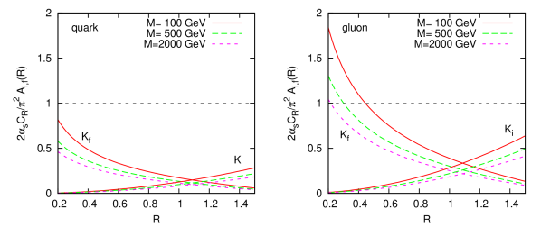
Figure 1: Coefficients $2\alpha_{a}C_{R}A_{i,f}(R)/\pi^{2}$, governing the behaviour of the initial or final-state QCD spectrum as a function of $R$ for different masses. The left plot covers the case of quark jets for which we use $C_{R}=C_{F}=4/3$, and the right plot is for gluon jets for which $C_{R}=C_{A}=3$.

Together with the spectrum, we will also need the total probability for the reconstructed mass to be within a certain range, i.e. the integrated spectrum. Denoting by $P(\delta m_{1},\delta m_{2})$ the probability for $m_{{\rm rec}}-M$ to be between $\delta m_{1}$ and $\delta m_{2}$, we easily find

$$P(\Lambda_{i,f},\delta m)=\left[\frac{\log(|\delta m|/\Lambda_{i,f})}{\log(M/(2\Lambda_{i,f}))}\right]^{K_{i,f}}$$ (11)

corresponding to the spectrum (9). Note that in this computation, we have assume that the spectrum is cut at the Landau pole, corresponding to $|\delta m|=\Lambda_{i,f}$.

Before proceeding with a more involved computation, it is important to comment on the limit of validity of this perturbative computation. From equations (3), (4) and (3.1), one might expect higher-order corrections to be important when $2\alpha_{s}C_{R}A_{i,f}(R)/\pi^{2}$ becomes of order 1. Fixing the scale in the coupling to $M/2$ for the sake of the argument, we have plotted that quantity on Fig. 1 for various cases of interest. In the case of quark-jets, both $K_{i}$ and $K_{f}$ remain smaller than 1. The case of gluon jets is more interesting; we see that the coefficient for final-state radiation goes above one at small $R$. In the case of a small-mass resonance, this can happen for values of $R$ as large as 0.5. As a rule of thumb, we can thus say that, in the case of a small-mass resonance decaying to gluon jets, our perturbative computation would only be valid for $R\gtrsim 0.5$. It is particularly interesting to relate that to the observation made in [4] that in this precise case of small-mass resonances decaying into gluons, we observed a disappearance of the peak in the reconstructed mass spectrum for small values of $R$. Though this was happening at slightly smaller values of $R$ (around $R\approx 0.4$), the present computation provides an explanation of this effect: when $2\alpha_{a}C_{R}A_{i,f}(R)/\pi^{2}$ grows above 1, the peak in the final-state radiation spectrum (9) is no longer around $z=0$ and the mass peak disappears. We shall come back to this point later in Section 4.2.

Note also that, from Fig. 1, one can have a feeling of what the optimal radius will be for parton-level events. Indeed, one can expect that, for $R=R_{\rm best}$, the spectrum will be nearly symmetric around the nominal mass (i.e. around $z=0$), that is $K_{i}(R_{\rm best})=K_{f}(R_{\rm best})$. For both quarks and gluons and for all masses, this means that one should expect $R_{\rm best}\approx 1.1$. We will see later on that this is indeed relatively close to what we shall obtain but that PDF effects, computed in the next Section, induce some departure from that situation.

3.2 PDF effects

In order to get a better description of the variety of processes we consider over the whole kinematic range, we shall see that it is important to take into account the effect of the PDF on initial-state radiation. This addresses the fact that the emission of an initial-state gluon imposes to take the parton distribution functions at a larger momentum fraction $x$. This should therefore introduce an additional suppression, more important at large mass and for gluon-jets than for quark jets.

Let us consider the production of a heavy particle at a fixed rapidity $y$. The leading-order cross section is easily obtained:

$$\sigma_{a}^{LO}(y) =\int{\rm d}x_{1}{\rm d}x_{2}\>f_{a}(x_{1})\,f_{a}(x_{2})\>\delta(x_{1}x_{2}s-M^{2})\,\delta\left(\frac{1}{2}\log\left(\frac{x_{1}}{x_{2}}\right)\!-y\!\right)\hat{\sigma}(M,y)$$

$$=\frac{1}{s}\,f_{a}\left(\frac{M}{\sqrt{s}}e^{y}\right)f_{a}\left(\frac{M}{\sqrt{s}}e^{-y}\right)\,\hat{\sigma}(M,y),$$ (12)

where the index $a$ represents the colour of the colliding partons, $f_{a}(x)$ is the PDF implicitly taken at a scale $M$, and $s$ is the centre-of-mass energy of the collision. This expression also comes with the kinematic constraint $|y|\leq\log(M/\sqrt{s})$.

We should now add to that process an extra parton emitted at a rapidity $\eta$. For our purpose of computing the initial-state radiation contamination to a jet, we can safely make the simplifying assumption that the rapidity of the gluon is the same as the rapidity of the “leading” parton, i.e., $\eta=y$. By doing so, we decouple the effects of the PDF from the effects of the jet clustering. The latter will be reinserted later on by multiplying our results by the geometric factor $A_{i}(R)$. We thus have

$$\sigma_{a}^{NLO}(y)=\frac{\alpha_{s}}{2\pi^{2}}\int{\rm d}x_{1}{\rm d}x_{2}{\rm d}\xi\,f_{a}(x_{1})f_{a}(x_{2})\,\frac{2C_{a}}{1-\xi}\,\delta(x_{1}x_{2}\xi s-M^{2})\,\delta\left(\frac{1}{2}\log\left(\frac{x_{1}\xi}{x_{2}}\right)\!-\!y\right)\hat{\sigma}.$$

In that expression, $\xi$ is the longitudinal fraction of $x_{1}$ carried by the parton entering the collision satisfying $1-\xi\ll 1$. If we rewrite it in terms of the longitudinal momentum of the emitted parton (measured w.r.t. the momentum of the beam) $\zeta=(1-\xi)x_{1}$, one gets after a bit of algebra

$$\frac{{\rm d}\sigma_{a}^{NLO}}{{\rm d}\zeta}(y)=\frac{1}{s}\,\frac{\alpha_{s}}{2\pi^{2}}\,f_{a}\left(\frac{M}{\sqrt{s}}e^{y}+\zeta\right)f_{a}\left(\frac{M}{\sqrt{s}}e^{-y}\right)\frac{2C_{a}}{\zeta}\hat{\sigma}.$$ (13)

Keeping the kinematic conventions introduced in the previous section, the longitudinal fraction $\zeta$ can be rewritten in terms of the transverse momentum $k_{t}=zM/2\approx\delta m$ of the parton as

$$\zeta=\frac{e^{y}}{\sqrt{s}}\,\delta m,$$ (14)

which finally implies

$$\frac{{\rm d}\sigma_{a}^{NLO}}{{\rm d}\delta m}(y)=\frac{1}{s}\,\frac{\alpha_{s}}{2\pi^{2}}\,f_{a}\left(\frac{(M+\delta m)e^{y}}{\sqrt{s}}\right)f_{a}\left(\frac{Me^{-y}}{\sqrt{s}}\right)\frac{2C_{a}}{\delta m}\hat{\sigma},$$ (15)

with the kinematic constraint

$$-\log\left(\frac{M}{\sqrt{s}}\right)\leq y\leq\log\left(\frac{M}{\sqrt{s}}\right)-\log\left(1+\frac{\delta m}{M}\right)$$ (16)

In the limit of small $\delta m$, i.e. neglecting the $\delta m$ offset in the PDF, one gets

$$\frac{{\rm d}\sigma_{a}^{NLO}}{{\rm d}\delta m}(y)\approx\frac{\alpha_{s}C_{R}}{\pi^{2}}\,\frac{1}{\delta m}\,\sigma_{a}^{LO}(y),$$

which is exactly the result we have obtained in the soft limit up to the geometric factor $2A_{i}(R)$ that we will need to reintroduce at the end of the computation.

To simplify the discussion, we shall assume that the PDFs take the form

$$f_{a}(x)=N_{a}\,x^{-\lambda-1}\,(1-x)^{\beta_{a}}.$$ (17)

The coefficients $N_{a}$ and $\beta_{a}$ will depend on the type of parton and the scale $M$ but we shall assume a unique value for $\lambda$.

At this level, we could proceed by integrating over the rapidity $y$. This is feasible analytically with the choice of PDF (17) but it leads to a Gauss hypergeometric function in ${\rm d}P^{(0)}_{i,f}/{\rm d}\delta m$ for which the Sudakov factor (8) cannot be computed analytically. We will therefore carry on with the computation at a fixed rapidity $y$.

Taking into account the emissions from both partons entering the collisions, normalising to the $LO$ cross-section and reinserting the geometric factor, one obtains

$$\frac{{\rm d}P_{i}^{(0)}}{{\rm d}\delta m}=\frac{\alpha_{s}C_{a}}{\pi^{2}}\,A_{i}(R)\,\frac{1}{\delta m}\tau^{-\lambda-1}\left[\left(\frac{1-\kappa\tau e^{y}}{1-\kappa e^{y}}\right)^{\beta_{a}}+\left(\frac{1-\kappa\tau e^{-y}}{1-\kappa e^{-y}}\right)^{\beta_{a}}\right],$$ (18)

where we have introduced $\kappa=M/\sqrt{s}$ and $\tau=1+\delta m/M$, and it is understood that the terms in the squared brackets are restricted to the appropriate phase space i.e. $\kappa\tau e^{\pm y}\leq 1$, respectively for each term.

In order to compute the Sudakov form factor analytically, we shall make the approximation that the exponents $\beta_{a}$ are integers (in practice, we shall use $\beta_{q}=3$ and $\beta_{g}=5$ for (anti-)quark and gluon-jets respectively), and expand the small-$x$ power behaviour to first order in $\delta m$:

$$\tau^{-\lambda-1}\approx 1-(1+\lambda)\frac{\delta m}{M}.$$ (19)

Using

$$\frac{1-\kappa\tau e^{\pm y}}{1-\kappa e^{\pm y}}=1-\frac{\kappa e^{\pm y}}{1-\kappa e^{\pm y}}\,\frac{\delta m}{M},$$ (20)

the fact that $\beta_{a}$ is an integer allows one to see (18) as a polynomial in $\delta m$.

We can then easily compute the Sudakov factor using the following fundamental integrals:

$$\int_{\delta m}^{M/2}\frac{{\rm d}u}{\log(u/\Lambda_{i})}\,u^{p-1} \overset{p=0}{=} \log\left[\frac{\log(M/(2\Lambda_{i}))}{\log(\delta m/\Lambda_{i})}\right],$$ (21)

$$\overset{p\neq 0}{=} \Lambda_{i}^{p}\left\{{\rm Ei}\left[p\,\log(M/(2\Lambda_{i}))\right]-{\rm Ei}\left[p\,\log(\delta m/\Lambda_{i})\right]\right\},$$ (22)

where ${\rm Ei}(x)$ is the exponential integral.

With these simplifying assumptions, the final perturbative spectrum for initial-state radiation can be written as

$$\frac{{\rm d}P_{i}}{{\rm d}\delta m}=\frac{K_{i}}{\log(\delta m/\Lambda_{i})}\,\left(\sum_{k=0}^{\beta_{a}+1}\mu_{k}\,\frac{\delta m^{k-1}}{M^{k}}\right)\,P_{i}(\Lambda_{i},\delta m)$$ (23)

with the integrated probability

$$P_{i}(\Lambda_{i},\delta m)=\left[\frac{\log(\delta m/\Lambda_{i})}{\log(M/(2\Lambda_{i}))}\right]^{K_{i}}\,\exp\left[-K_{i}\sum_{k=1}^{\beta_{a}+1}\mu_{k}\,{\cal E}_{k}\left(\frac{\Lambda_{i}}{M}\right)^{k}\right],$$ (24)

and the coefficients

$$\mu_{k} = \nu_{k}-(1+\lambda)\nu_{k-1},$$ (25)

$$\nu_{k} = \frac{1}{2}C_{\beta_{a}}^{k}\left[\left(\frac{\kappa}{\kappa\!-\!e^{-y}}\right)^{k}\,\Theta\!\left(\frac{\kappa\!-\!e^{-y}}{\kappa}\!-\!\frac{\delta m}{M}\right)+\left(\frac{\kappa}{\kappa\!-\!e^{y}}\right)^{k}\,\Theta\!\left(\frac{\kappa\!-\!e^{y}}{\kappa}\!-\!\frac{\delta m}{M}\right)\right],$$ (26)

$$\nu_{-1} = \nu_{\beta_{a}+1}=0,$$ (27)

$${\cal{E}}_{k} = {\rm Ei}\left[k\,\log(M/(2\Lambda_{i}))\right]-{\rm Ei}\left[k\,\log(\delta m/\Lambda_{i})\right].$$ (28)

Note that to obtain (28), we have to integrate $\delta m$ up to $M/2$, which is strictly valid only when $|y|\leq\log(\kappa/2)$, but similar results can easily be derived at forward rapidities.

3.3 Comparison with Monte Carlo

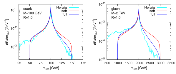
Figure 2: Reconstructed mass spectrum from our perturbative-QCD computation compared with Herwig at parton level (cyan curve). For the analytic computation, we show both the soft approximation (red curve) and the full case including PDF effects (blue curve). The left plot is for a $q\bar{q}$ dijet system at a nominal mass of 100 GeV while the right plot is for the gluonic case at 2 TeV. In both cases, the anti-$k_{t}$ algorithm with a radius of 1 has been used for the clustering.

We want to conclude this Section by a comparison of the predictions we obtain for the optimal radius from our analytical studies and from Monte-Carlo approaches. When dealing with the analytic result, we shall use the initial and final-state results computed in the previous sections in the two different situations for which we have analytic results: the soft limit with a running-coupling approximation, eqs. (9) and (11), and the “full” spectrum where we also include the PDF effects in the initial-state radiation, eq. (23).

The total perturbative QCD spectrum is the convolution of the initial and final-state pieces which, in practice, will be carried numerically. We shall use $\Lambda_{\rm QCD}=200$ MeV and $N_{f}=5$ to compute the running of the QCD coupling, and, for the PDF effects in the initial-state-radiation spectrum, we shall adopt $\lambda=0.3$, $\beta_{q}=3$ and $\beta_{g}=5$, and assume $y=0$, where we have checked that most of the massive objects in the Monte Carlo sample were produced. The quality measure is computed from the spectrum using (1).

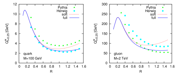
Figure 3: Quality measure as a function of $R$ for the parton-level spectrum. The (red) dashed curve corresponds to our analytic computation in the soft limit while the (blue) solid one includes PDF effects. The (green) triangles and (cyan) circles show the Monte-Carlo simulations for Pythia and Herwig respectively. As for Fig. 2, the left plot is for a $q\bar{q}$ dijet system at a nominal mass of 100 GeV while the right plot is for the gluonic case with $M=2$ TeV.

We start our comparison directly with the spectrum for the reconstructed dijet mass, as shown on Fig. 2 for quark jets, $M=100$ GeV and gluon jets, $M=2$ TeV. Generally speaking, the agreement between our analytic computation and Herwig is good, even very good for the 100 GeV quark-jet case. Note that this agreement is always better in the region of the peak, where the soft-gluon emissions approximation we are working with is supposed to hold. Similarly the small differences in the tail at small and large $m_{{\rm rec}}$ are beyond the scope of our approximation. In both the quark and gluon-jet cases, we see that the inclusion of PDF effects, reducing the initial-state radiation, significantly improves the description, especially in the case of large-mass gluon jets, where we are sensitive to fast-falling gluon distributions at large $x$.

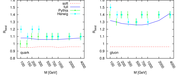
Figure 4: Best radius as a function of the mass, obtained from our analytic computation and compared to Monte-Carlo results. The analytic curves correspond to the soft limit (dotted red curve), and full computation (solid blue curve). These are compared to values of $R_{\rm best}$ extracted from parton-level Pythia (green triangles) and Herwig (cyan circles) simulations. The left plot shows the case of a resonance decaying into $q\bar{q}$ jets while the right plot has gluon jets.

Next, we turn to the computation of the quality measure, presented in Fig. 3. After properly taking into account the PDF effects, our computation agrees in shape with the Monte-Carlo results. For the normalisation, we are closer to the Herwig simulation in the case of quark jets, while we better agree with Pythia simulations for gluon jets. Since our analytic computation is identical in both cases, it it somehow hard to find an explanation for those differences.

Finally, let us concentrate on the values of $R_{\rm best}$ extracted from the previous examples. This is shown on Fig. 4 for quark jets (left panel) and gluon jets (right panel). Despite the apparent normalisation issue between Pythia and Herwig observed on Fig. 3, the fact that they agree on the shape of the quality means that they yield very similar extracted optimal radii. If we turn to the analytic computation, we first see that in the soft approximation, the optimal radius is independent on the process under consideration with $R_{\rm best}\approx 0.96$ regardless of the mass or the parton type. The reduction of the initial-state radiation due to the PDF effects has a sizeable effect on the extracted optimal radius in such a way that, at the end of the day, our analytic extraction of $R_{\rm best}$ in the “full” model reproduces very well the Monte-Carlo simulations with an error $\lesssim$ 0.1.

4 Effects of the Underlying Event

4.1 Description of the Underlying Event

One of the most important effects when clustering jets at hadronic colliders is the presence of the underlying event (UE) coming from multiple interaction and beam remnants. This tends to produce a fairly uniform soft radiation of a few GeV per unit area that contaminates the jets and affects their momentum reconstruction. In this Section, we therefore study the effects of this UE on the mass spectrum we have computed from perturbative QCD in the previous Section.

If we work within the assumption that the UE is uniform in rapidity and azimuth, the average $p_{t}$ contamination to each jet will be ${\cal A}_{\rm jet}\rho$ where ${\cal A}_{\rm jet}$ is the (active) area of the jet [22] and $\rho$ the UE density per unit area. For a given event, this contamination is affected by two kinds of fluctuations: first, the fluctuations of the background itself which go like $\sqrt{{\cal A}_{\rm jet}}\sigma$, with $\sigma$ the background fluctuations per unit area. Then, keeping in mind the possibility to discuss our results for different jet algorithms than the anti-$k_{t}$ algorithm, the active area of a jet is in general known to fluctuate, with an average value proportional to $\pi R^{2}$ that increases with $p_{t}$ in a different way for each jet algorithm.

For a given background density $\rho$, let us denote by ${\rm d}P_{i}/{\rm d}p_{t,k}$ the probability distribution for a jet $k$ to receive a contamination $p_{t,k}$ from the UE. For a jet of area ${\cal A}_{\rm jet}=\pi R^{2}\,a_{k}$, this distribution has an average of $\pi R^{2}\,a_{k}\rho$ and a dispersion $\sqrt{\pi R^{2}\,a_{k}}\sigma$. We therefore also have to introduce ${\rm d}P_{a}/{\rm d}a_{k}$ the distribution, of average $\bar{a}$ and dispersion $\sigma_{a}$ of the area divided by $\pi R^{2}$, of the jet $k$.

If the two jets were perfect circles of radius $R$, one could easily compute that the offset on the reconstructed mass would be $\delta m=2\pi RI_{1}(R)(\rho_{1}+\rho_{2})$, up to corrections proportional to $\delta m^{2}/M$, where $I_{1}(x)$ is the modified Bessel function of the first kind. For generic jets we shall then use

$$\delta m=\frac{2I_{1}(R)}{R}(p_{t,1}+p_{t,2}),$$ (29)

where $p_{t,1}$ and $p_{t,2}$ are the transverse momenta of the background contamination of our dijets.

On top of that, when we consider an event sample, the values of $\rho$ and $\sigma$ will fluctuate from one event to another. For the event-by-event fluctuations of the background densities, we shall assume a distribution ${\rm d}P_{e}/{\rm d}\rho$, of average $\left\langle\rho\right\rangle$ and dispersion $\sigma_{\rho}$. For the intra-event fluctuations (per unit area) $\sigma$ we shall simply assume that they remain proportional to $\rho$, i.e., $\mu=\sigma/\rho=\left\langle\sigma/\rho\right\rangle$.

Given the event-by-event $\rho$ distribution ${\rm d}P_{e}/{\rm d}\rho$, the intra-event fluctuations, ${\rm d}P_{i}/{\rm d}p_{t,k}$ and the area distribution ${\rm d}P_{a}/{\rm d}a_{k}$, the UE spectrum can be inferred from (29)

$$\frac{{\rm d}P_{\rm UE}}{{\rm d}\delta m}=\int{\rm d}\rho\frac{{\rm d}P_{e}}{{\rm d}\rho}\int{\rm d}a_{1}{\rm d}a_{2}\frac{{\rm d}P_{a}}{{\rm d}a_{1}}\frac{{\rm d}P_{a}}{{\rm d}a_{2}}\,\int{\rm d}p_{t,1}{\rm d}p_{t,2}\frac{{\rm d}P_{i}}{{\rm d}p_{t,1}}\frac{{\rm d}P_{i}}{{\rm d}p_{t,2}}\delta\left(\delta m-\frac{2I_{1}(R)}{R}(p_{t,1}+p_{t,2})\right).$$ (30)

Without knowing exactly that distribution, we can compute its average and dispersion in terms of the properties of the fundamental distributions:

$$\left\langle\delta m\right\rangle = \int{\rm d}\delta m\,\delta m\,\frac{{\rm d}P_{\rm UE}}{{\rm d}\delta m}$$

$$= \left[\frac{2I_{1}(R)}{R}\right]\,2\pi R^{2}\bar{a}\,\left\langle\rho\right\rangle,$$

$$\sigma_{\delta m}^{2} = \int{\rm d}\delta m\,(\delta m-\left\langle\delta m\right\rangle)^{2}\,\frac{{\rm d}P_{\rm UE}}{{\rm d}\delta m}$$

$$= \left[\frac{2I_{1}(R)}{R}\right]^{2}\left[4\bar{a}^{2}(\pi R^{2})^{2}\sigma_{\rho}^{2}+2(\pi R^{2})^{2}\left(\left\langle\rho\right\rangle^{2}+\sigma_{\rho}^{2}\right)\sigma_{a}^{2}+2\bar{a}(\pi R^{2})\left(\left\langle\rho\right\rangle^{2}+\sigma_{\rho}^{2}\right)\mu^{2}\right].$$

The average is consistent with what one would naively expect, and the dispersion is a combination of the three separate sources of dispersion we are including: event-by-event fluctuations in $\rho$ (the first term), area fluctuations (the second term) and intra-event fluctuations (the third term). As expected, the first two are proportional to the area of the jet i.e. to $\pi R^{2}$, while the intra-event fluctuations are proportional to its square root.

So, instead of modelling the various distributions separately and perform the integrations in (30), we shall directly model the total UE spectrum and adjust its parameters to reproduce the total average and dispersion. More specifically, we shall assume

$$\frac{{\rm d}P_{UE}}{{\rm d}\delta m}=\frac{1}{\Gamma(\alpha)}\frac{\delta m^{\alpha-1}}{\delta m_{0}^{\alpha}}e^{-\delta m/\delta m_{0}}.$$ (33)

The parameters $\delta m_{0}$ and $\alpha$ can be adjusted to reproduce the average (4.1) and dispersion (4.1) of the UE distribution. One finds

$$\alpha=\frac{\left\langle\delta m\right\rangle^{2}}{\sigma_{\delta m}^{2}}\qquad\text{ and }\qquad\delta m_{0}=\frac{\sigma_{\delta m}^{2}}{\left\langle\delta m\right\rangle}.$$ (34)

This choice has the advantage over a Gaussian distribution that it remains positive.

4.2 Computation and comparison with Monte Carlo

Our strategy is rather straightforward: as we did when combining the initial-state and final-state radiation spectra, we shall convolute the perturbative QCD spectrum, discussed in Section 3.3, with the UE spectrum (33). For each mass and parton-type, we wish to compare our results with the Monte-Carlo studies [4].

For the perturbative QCD part of the spectrum, we use the convolution already discussed in Section 3.3 and consider the same models: the pure soft approximation and the spectrum including PDF effects in the initial-state. The result is itself convoluted with the underlying-event distribution for which we still have to determine the parameters appearing in eqs. (4.1) and (4.1). The area properties $\bar{a}$ and $\sigma_{a}$ have been calculated, together with their scaling violations in [22]. The properties of the background are computed directly from the Monte-Carlo event sample using FastJet [24] and the method advocated in [25] and [23]: each event is first clustered with the Cambridge/Aachen algorithm with $R=0.6$; $\rho$ and $\sigma$ are then estimated from the jets that are within a rapidity strip of 1 unit around the hardest dijet system, excluding the two hardest jets in the event. The average properties $\left\langle\rho\right\rangle$, $\mu$ and $\sigma_{\rho}$ can then be easily extracted from the complete event sample. For completeness, we give a table of the values we have obtained in Appendix A.

With that method, we are able to compute the mass spectrum, and thus the quality measure, at a given mass and with a given parton type and UE characteristics. We then extract $R_{\rm best}$ by searching the minimum of the quality measure by steps of 0.01 in $R$.

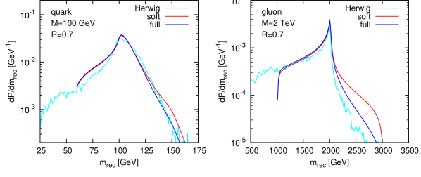
Figure 5: Reconstructed mass distribution for quark dijets at 100 GeV (left panel) and gluon dijets at 2 TeV (right panel). We compare the Monte-Carlo simulations from Herwig with our analytic computation. In both cases, we have used $R=0.7$ and the anti-$k_{t}$ algorithm.

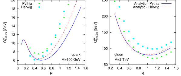
Figure 6: Quality measures as a function of $R$ for quark dijets at 100 GeV (left panel) and gluon dijets at 2 TeV (right panel). The triangles and solid lines correspond to the Pythia simulations while the circles and dashed lines correspond to Herwig simulations.

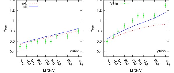
Figure 7: Best radius as a function of the mass when including the UE. Our analytic results are compared with Pythia Monte-Carlo simulations. The left (right) plot is for quark (gluon) jets.

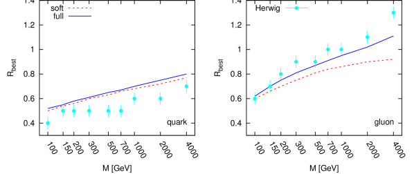
Figure 8: Same as Fig. 7 but for Herwig simulations.

As for the parton-level case, we shall compare our computations with the Monte Carlo simulations from Pythia (tune DWT) and Herwig (with default Jimmy tune) as the details of the Underlying Event can differ. We shall again proceed in three steps: first consider the histograms, then the quality measures and finally the optimal radius. For simplicity, we shall focus on the anti-$k_{t}$ algorithm for which $\bar{a}=1$ and $\sigma_{a}^{2}=0$.

Let us start with the histograms, Figure 5, where we illustrate our description of the spectrum for the quark dijets at small mass and gluon dijets at large mass. In both cases, our analytic histogram correctly reproduces the behaviour observed with Herwig. We note however that our analytic computation slightly underestimating the UE in the peak region in the case of quark jets at small nominal mass $M$. If we then move to the case of the quality measure, Figure 6, we see that, given the differences we have already observed at the parton level (see Figure 3), the addition of the underlying event gives a reasonable description of the Monte-Carlo results, especially the shape of the quality at large $R$. Note that only the curves corresponding to the model including the PDF effects are shown on Figure 6 for clarity reasons.

Finally, the extracted optimal radius is presented on Figures 7 and 8 for Pythia and Herwig simulations respectively, as a function of the mass for both quark and gluon jets. Generally speaking we obtain a good description of the Monte-Carlo results. We see once again that the inclusion of the PDF effects significantly improves the description of the optimal radius for gluon jets at large mass, as expected. We slightly underestimate the optimal radius in the case of gluon jets at large mass, but we have to notice that this is the regime on which it matters the least as in that region the minimum in the quality measure is rather flat.

We thus see that our complete analytic model, the solid (blue) curve on Figures 7 and 8, corresponding to our analytic pQCD computation including PDF effects, eq. (23), convoluted with our model of the Underlying Event, eq. (33), gives a good extraction of the optimal radius $R_{\rm best}$.

4.3 Computation for other algorithms

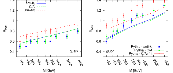
Figure 9: Best radius as a function of the mass for different algorithms. The lines are obtained using our analytic approach while the points correspond to Pythia simulations. The left plot shows the case of quark dijets and gluons are shown on the left panel. The solid (blue) lines together with the squares correspond to the anti-$k_{t}$ results, the dashed (green) lines and the circles show C/A results, and the dotted (red) lines and the triangles correspond to C/A with filtering.

Now that we have checked the agreement between our analytic computations and Monte-Carlo simulations for the simpler case of the anti-$k_{t}$ algorithm, let us briefly discuss other possible jet algorithms. In this section, we shall apply our analytic computations to the case of the Cambridge/Aachen (C/A) as well as to the Cambridge/Aachen algorithm supplemented by a filter (C/A+filt). While the former usually leads to quality measurements close to what is obtained in the anti-$k_{t}$ case, the latter produces narrower peaks with an optimal radius slightly larger than the one obtained from C/A without filtering. For simplicity, we shall follow what has been done in [4] and use $R_{\rm filt}=R/2$ and $n_{\rm filt}=2$ for the parameters of the filter, i.e., recluster each jet with C/A and a radius of half the original one and keep the two hardest subjets, discarding the softer ones.

The analytic computation goes exactly as in the case of the anti-$k_{t}$ algorithm. The only thing that will change in our approach is the inclusion of the area contribution in the UE distribution. The expressions for the area are computed analytically, as in [22], up to order $\alpha_{s}$:

$$\bar{a} = A_{0,{\rm JD}}+d_{{\rm JD}}\,\frac{C_{a}}{\beta_{0}\pi}\log\left[\frac{\alpha_{s}(Q_{0,{\rm JD}}^{(a)})}{\alpha_{s}(Rp_{t})}\right],$$ (35)

$$\sigma_{a}^{2} = \Sigma_{0,{\rm JD}}^{2}+s_{{\rm JD}}^{2}\,\frac{C_{a}}{\beta_{0}\pi}\log\left[\frac{\alpha_{s}(Q_{0,{\rm JD}}^{(a)})}{\alpha_{s}(Rp_{t})}\right],$$ (36)

where the coefficient $A_{0}$, $d$, $\Sigma_{0}$ and $s$ are computed in perturbation theory and have been calculated in [22], while the scales $Q_{0}$ are of non-perturbative origin and have been determined in [22] from a fit to Herwig simulations. In our case, we shall use $p_{t}=M/2$ together with the following values for the coefficients :

$$A_{0,{\rm C/A}}=0.814,\quad d_{\rm C/A}=0.083, \Sigma_{0,{\rm C/A}}^{2}=0.0687,\quad s_{\rm C/A}^{2}=0.036,$$ (37)

$$A_{0,{\rm C/A+filt}}=0.386,\quad d_{\rm C/A+filt}=0.019, \Sigma_{0,{\rm C/A+filt}}^{2}=0.0046,\quad s_{\rm C/A+filt}^{2}=0.004,$$ (38)

$$Q_{0,{\rm C/A}}^{(q)}=Q_{0,{\rm C/A+filt}}^{(q)}=0.26\text{ GeV}, Q_{0,{\rm C/A}}^{(g)}=Q_{0,{\rm C/A+filt}}^{(g)}=0.53\text{ GeV}.$$ (39)

To avoid multiplying the figures, we just show, see Figure 9, the final result of the extracted optimal radius as a function of the mass for the three algorithms under consideration, compared to Pythia simulations. We see that, in agreement with the Monte Carlo, the differences between anti-$k_{t}$ and Cambridge/Aachen are very small and thus our analytic approach reproduces the expected behaviour correctly. For the case of the C/A algorithm with filtering, we obtain a good description in the case of quark dijet systems but systematically underestimate the optimal radius, by about 0.1-0.2, in the case of gluon jets. We believe that this is due to the fact that we should also introduce some dependence on the algorithm at the level of the perturbative spectrum. In our soft-gluon approximation all the algorithm will have the same initial and final-state radiation spectra. However, with a more complete treatment, e.g. including non-global logarithms as in [19], differences will start appearing. Another effect comes from the combination of the initial and final-state radiation spectra: the simple convolution we have used is reasonable in the case of the anti-$k_{t}$ algorithm where the shape of the jet is not affected by the radiation, but more subtle phenomena will appear for more complex algorithms, especially in the filtered case where, in some geometric regions, the capture of ISR gluons can be affected by internal gluon radiation in the jet.

All these effects are beyond the reach of the present analysis. As expected from the previous discussion, discrepancies are more pronounced in the case of gluon jets at large mass, where perturbative radiation dominated the spectrum. Our computation nevertheless gives reasonable results at the end of the day, given also that for gluon dijets at larger mass, the minimum in the quality measure is less pronounced than in other situations.

Finally, let us mention that the case of the $k_{t}$ algorithm [21] is also very close to what we obtain for the anti-$k_{t}$ and C/A algorithm, hence well reproduced by our calculation. For the SISCone algorithm, differences in the perturbative spectrum also appear when the radiated gluon is not soft, we therefore postpone that case for a further study.

4.4 Comparison with earlier approaches

To some extent, the present calculation can be seen as an extended version of what has been done in [13], where the authors compute the average $p_{t}$ shift of a jet due to final-state radiation, hadronisation and the UE. The approach we pursue in this paper is however much more complete in the sense that we obtain the full spectrum instead of just the average value. As a consequence, we can extract the width of the peak really as the dispersion in the spectrum, while in [13] the width is approximated by

$$\left\langle\delta p_{t}^{2}\right\rangle\approx\left\langle\delta p_{t}\right\rangle_{\rm pert}^{2}+\left\langle\delta p_{t}\right\rangle_{\rm hadr}^{2}+\left\langle\delta p_{t}\right\rangle_{\rm UE}^{2}$$ (40)

i.e. the total dispersion is approximated by the sum of each independent average squared. The individual contributions are found to be [13]

$$\left\langle\delta p_{t}\right\rangle_{\rm pert} = \frac{\alpha_{s}}{\pi}\log(R)L_{a}p_{t},$$

$$\left\langle\delta p_{t}\right\rangle_{\rm hadr} = \frac{-2C_{a}}{R}{\cal A}(\mu_{I}),$$ (41)

$$\left\langle\delta p_{t}\right\rangle_{\rm UE} = \Lambda_{\rm UE}\,RJ_{1}(R)$$

with $2C_{F}{\cal A}(\mu_{I})=0.5$ GeV for $\mu_{I}=2$ GeV and

$$L_{q} = \left(2\log(2)-\frac{3}{8}\right)C_{F},$$

$$L_{g} = \left(2\log(2)-\frac{43}{96}\right)C_{A}+\frac{7}{48}N_{f}T_{R}.$$

The optimal radius is then obtained by minimising (40) w.r.t. $R$.

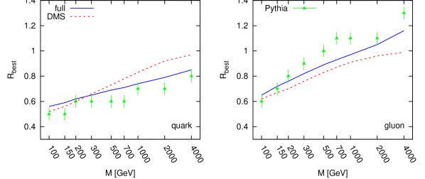
Figure 10: Best radius as a function of the mass for our approach compared to the previous work of [13]. The solid (blue) line corresponds to our present computation in this paper while the dotted (red) line shows the result obtained in Ref. [13]. The Pythia results, the (green) triangles, are shown for comparison. The left (right) panel shows the case of quark (gluon) jets.

In practice, we have used $p_{t}=M/2$, $N_{f}=5$, $\Lambda_{\rm QCD}=200$ MeV and computed the QCD coupling at the scale $Rp_{t}$. Instead of using a fixed value for $\Lambda_{\rm UE}$ as in [13], we have used the fact that it is related to the average background density, $\left\langle\rho\right\rangle$, through (see Section 4.1)

$$\Lambda_{\rm UE}=2\pi\bar{a}\left\langle\rho\right\rangle\frac{I_{1}(R)}{J_{1}(R)},$$ (43)

and used the values extracted from the Monte Carlo event samples and already used in Section 4.1 for $\left\langle\rho\right\rangle$.

The extracted value of $R_{\rm best}$ is shown on Fig. 10 in the case of Pythia simulations, for the anti-$k_{t}$ algorithm. The results are compared with the Monte Carlo results and with our complete analytic calculation. We see that the simpler approach of [13] manages to extract the correct value for $R_{\rm best}$ at small mass but fails to reproduce the observed behaviour at larger mass, and this for both quark and gluon jets. The reason for this failure is rather hard to pinpoint: it can come, e.g., from the crudeness of the approximation (40), the lack of an initial-state radiation contribution and the corresponding PDF effects, or the description of the underlying event in terms of the average density $\left\langle\rho\right\rangle$ instead of its fluctuations $\sigma_{\rho}$.

5 Background subtraction

5.1 Description

The last point we wish to discuss is the situation where we perform background subtraction using jet areas [22], as advocated in [25]. The idea behind UE subtraction is to get rid of the shift due to the UE density contaminating the mass reconstruction. Since subtraction is performed on each single event, one hopes to get rid of the fluctuations of the background density across the events, hence obtaining a narrower peak. In this respect, all we should be left with is the background fluctuations inside an event which have a linear dependence on $R$ rather than the quadratic one computed in the unsubtracted case (4.1). This is a much smaller effect and one thus expect the quality measure to be better (i.e. smaller) than in the unsubtracted case as well as the optimal radius to be larger.

In practice, one would thus naively convolute the perturbative spectrum computed in Section 3 with a subtracted UE spectrum taking into account these intra-event fluctuations. Doing that would actually lead to a quality much better than what is observed in Monte-Carlo studies and to a systematic over-estimation of $R_{\rm best}$.

The additional effect that is mandatory to take into account is the fact that subtraction is performed using an estimated value for the background density $\rho_{\rm est}$ which can differ from the exact value of $\rho$ for that event. This results in some smearing effect left over from the unsubtracted spectrum. Because of this, the computation of the subtracted UE spectrum turns out to be more involved than the corresponding unsubtracted case computed in Section 4.1, mostly because one also would have to consider the distribution probability for $\rho_{\rm est}$.

The properties of the estimated value of $\rho$ have actually recently been discussed at length in [23], where we learn that the estimation of the background density using a median-based approach suffers from two sources of bias: one of soft origin, related to the fact that the median of a set of pure-UE jets may differ from its average; and a contamination from radiation coming from the hard jets. If we call $\rho$ and $\sigma$ the average UE density and its fluctuations for one given event, and define $\delta=(\rho_{\rm est}-\rho)/\rho$ as the relative error in the estimation of $\rho$, the average and dispersion of $\delta$ are [23]

$$\left\langle\delta\right\rangle\simeq d_{1}\mu-d_{2}\mu^{2}\quad\text{ and }\quad\sigma_{\delta}^{2}\simeq S_{d}^{2}\mu^{2}$$ (44)

where, as in Section 4.1 we used $\mu=\sigma/\rho$, and the coefficients are

$$d_{1} = R_{\rho}\sqrt{\frac{\pi c_{J}}{2}}\left(\frac{\left\langle n_{h}\right\rangle}{A_{\rm tot}}+c_{J}R_{\rho}^{2}\frac{\left\langle n_{h}\right\rangle^{2}}{2A_{\rm tot}^{2}}\right),$$ (45)

$$d_{2} = \frac{1}{4c_{J}^{2}R_{\rho}^{2}}$$ (46)

and

$$S_{d}^{2}=\frac{\pi}{2A_{\rm tot}}+2\pi c_{J}R_{\rho}^{2}\frac{\left\langle n_{h}\right\rangle}{A_{tot}^{2}},$$ (47)

with

$$\left\langle n_{h}\right\rangle=A_{\rm tot}\frac{C_{a}}{2\pi^{2}\beta_{0}}\log\left(\frac{\alpha_{s}({\rm min}(Q_{0},\sqrt{c_{J}\sigma R_{\rho}}))}{\alpha_{s}(Q)}\right).$$ (48)

In the previous set of equations, $c_{J}\simeq 2.04$ is a pure number extracted in [23], $R_{\rho}$ is the jet radius used to estimate the background properties, $A_{\rm tot}$ is the total area of the range we are using to estimate the background, $Q_{0}$ is a soft cut-off that we fixed to 1 GeV, and $Q$ is the hard scale that we naturally took equal to $M/2$.

These properties constrain the distribution of $\delta$, that we shall denote by ${\rm d}P_{\delta}/{\rm d}\delta$, as a function of $\mu$. Since the intra-event fluctuations will play a substantial role in this UE-subtracted situation, we shall also consider a distribution for them. For simplicity, we shall parametrise the distribution in terms of $\mu$ rather than in terms of $\sigma$ as background estimations are naturally expressed in that variable. We therefore introduce ${\rm d}P_{\mu}/{\rm d}\mu$, of average $\left\langle\mu\right\rangle$ and dispersion $\sigma_{\mu}^{2}$. In the course of the computation below, we shall encounter higher cumulants for this distribution. To keep things simple, we shall work with the Gaussian assumption i.e. $\left\langle\mu^{3}\right\rangle=\left\langle\mu\right\rangle(\left\langle\mu\right\rangle^{2}+3\sigma_{\mu}^{2})$, $\left\langle\mu^{4}\right\rangle=\left\langle\mu\right\rangle^{4}+6\left\langle\mu\right\rangle^{2}\sigma_{\mu}^{2}+3\sigma_{\mu}^{4}$. The values of $\left\langle\mu\right\rangle$ and $\sigma_{\mu}^{2}$ can again be extracted from the Monte-Carlo samples.

With this at hand, we proceed, as in Section 4.1, by computing the mass shift for a given configuration and deducing its average and dispersion. For given values of $\rho$, $\mu$, $\rho_{\rm est}$, jet areas $a_{k}$ and jet UE contaminations $p_{t,k}$, the offset in the reconstructed mass after subtraction is

$$\delta m=\left[\frac{2I_{1}(R)}{R}\right]\left[p_{t,1}+p_{t,2}-\pi R^{2}(a_{1}+a_{2})(1+\delta)\rho\right],$$ (49)

where the last term is the subtracted piece.

After a slightly lengthy computation we reach

$$\left\langle\delta m\right\rangle = \left[\frac{2I_{1}(R)}{R}\right]\,2\pi R^{2}\bar{a}\,\left\langle\rho\right\rangle\left[-d_{1}\left\langle\mu\right\rangle+d_{2}(\left\langle\mu\right\rangle^{2}+\sigma_{\mu}^{2})\right],$$ (50)

$$\sigma_{\delta m}^{2} = \left[\frac{2I_{1}(R)}{R}\right]^{2}\left(\left\{\left[2\pi R^{2}\bar{a}+2(\pi R^{2})^{2}\sigma_{a}^{2}(d_{1}^{2}+S_{d}^{2})+4(\pi R^{2}\bar{a})^{2}S_{d}^{2}\right](\left\langle\rho\right\rangle^{2}+\sigma_{\rho}^{2})\right.\right.$$ (51)

$$\phantom{\left[\frac{2I_{1}(R)}{R}\right]^{2}()}\left.+4(\pi R^{2}\bar{a})^{2}d_{1}^{2}\sigma_{\rho}^{2}\right\}(\left\langle\mu\right\rangle^{2}+\sigma_{\mu}^{2})$$

$$\phantom{\left[\frac{2I_{1}(R)}{R}\right]^{2}}\left.+\left[2(\pi R^{2})^{2}\sigma_{a}^{2}(\left\langle\rho\right\rangle^{2}+\sigma_{\rho}^{2})+4(\pi R^{2}\bar{a})^{2}\sigma_{\rho}^{2}\right]\left(d_{2}^{2}\left\langle\mu^{4}\right\rangle-2d_{1}d_{2}\left\langle\mu^{3}\right\rangle\right)\right.$$

$$\phantom{\left[\frac{2I_{1}(R)}{R}\right]^{2}}\left.+\,4(\pi R^{2}\bar{a})^{2}\left\langle\rho\right\rangle^{2}\left[2d_{2}^{2}\sigma_{\mu}^{2}+(2d_{2}\left\langle\mu\right\rangle-d_{1})^{2}\right]\sigma_{\mu}^{2}\right).$$

Once we have these expressions, the last step is to parametrise the subtracted UE spectrum. Since subtraction can produce negative values for $\delta m$, we cannot use (33). The technique we shall adopt is to keep the same distribution using the unsubtracted average together with the dispersion we have just computed, and then to shift the complete distribution in order to reproduce the subtracted average $\delta m$. In practice, this gives

$$\frac{{\rm d}P_{UE,{\rm sub}}}{{\rm d}\delta m}=\frac{1}{\Gamma(\alpha)}\frac{(\delta m+\delta m_{1})^{\alpha-1}}{\delta m_{0}^{\alpha}}e^{-(\delta m+\delta m_{1})/\delta m_{0}}.$$ (52)

where the parameters $\delta m_{0}$, $\delta m_{1}$ and $\alpha$ are given by

$$\alpha=\frac{\left\langle\delta m\right\rangle_{\rm unsub}^{2}}{\sigma_{\delta m}^{2}},\qquad\delta m_{0}=\frac{\sigma_{\delta m}^{2}}{\left\langle\delta m\right\rangle_{\rm unsub}}\qquad\text{ and }\qquad\delta m_{1}=\left\langle\delta m\right\rangle_{\rm unsub}-\left\langle\delta m\right\rangle.$$ (53)

with $\left\langle\delta m\right\rangle$ and $\sigma_{\delta m}^{2}$ given by eqs. (50) and (51), and $\left\langle\delta m\right\rangle_{\rm unsub}$ by eq. (4.1).

Finally, it is interesting to notice that in the case of a perfect estimation of the background density $\rho_{\rm est}=\rho$, i.e. $d_{1}=d_{2}=S_{d}=0$, one recovers

$$\left\langle\delta m\right\rangle = 0,$$ (54)

$$\sigma_{\delta m}^{2} = \left[\frac{2I_{1}(R)}{R}\right]^{2}\,2\pi R^{2}\bar{a}(\left\langle\rho\right\rangle^{2}+\sigma_{\rho}^{2})(\left\langle\mu\right\rangle^{2}+\sigma_{\mu}^{2})$$ (55)

i.e. no average shift and a (squared) dispersion that is proportional to the area (linearly) and to $\sigma^{2}$.

5.2 Comparison with Monte-Carlo simulations

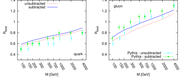
Figure 11: Best radius as a function of the mass for both the UE-unsubtracted and the UE-subtracted cases. The solid (blue) line corresponds to our subtracted prediction and has to be compared to the Pythia Monte-Carlo simulation shown as (green) circles. For reference, we also show as a (red) dotted line the unsubtracted predictions, together with the Pythia results shown as the (cyan) triangles. The left (right) panel shows the case of quark (gluon) jets.

As for the previous cases we have analysed, we shall perform a comparison of our analytic predictions with Monte Carlo simulations for the UE-subtracted case. The method goes exactly as before, so we just highlight the main steps and present our results for the optimal radius $R_{\rm best}$ and stay with the anti-$k_{t}$ algorithm.

For the analytic part of the computation, the perturbative QCD spectrum is convoluted with the subtracted UE spectrum calculated in the previous Section. Concerning the parameters of the latter, all background properties, $\left\langle\rho\right\rangle$, $\sigma_{\rho}^{2}$, $\left\langle\mu\right\rangle$ and $\sigma_{\mu}^{2}$ are extracted directly from the Monte-Carlo data sample and the estimation of the background density was performed using the Cambridge/Aachen algorithm with a radius of 0.6. We have kept all the jets within one unit of rapidity around the hardest dijet, excluding the two hardest jets in the event, giving a total area $A_{\rm tot}=4\pi$. It is interesting to notice that when background subtraction is performed, the final results will slightly depend on the details of how $\rho$ is estimated, through the coefficients $d_{1}$, $d_{2}$ and $S_{d}$ in our analytic approach. Extending the range, i.e. increasing its area $A_{\rm tot}$, would decrease the bias in the estimation of $\rho$, but in that case, there would be a risk that the background would not be uniform over the range (e.g. vary with rapidity). Following [23], we could therefore also try to optimise the choice of range and jet definition used for estimating $\rho$.

The computed value of $R_{\rm best}$ is shown on Fig. 11 in the case of Pythia simulations. For an easier comparison, we show both the subtracted and unsubtracted results. For the analytic calculation, we observe a value of $R_{\rm best}$ larger in the subtracted case by about 0.04 in the case of quark-jets and by about 0.08 in the case of gluon-jets. All these values are in good agreement with what is observed in the Monte-Carlo simulations.

6 Conclusions and perspectives

Throughout this paper we have investigated analytically the optimisation of the radius $R$ one uses with a jet algorithm to reconstruct dijet resonances. We have already learnt [4] that carefully choosing the jet radius can lead to significant improvement of the reconstructed signal and we find it valuable to supplement previous Monte-Carlo studies with an analytic understanding of these dijet reconstructions.

Our approach has been to calculate the reconstructed dijet mass spectrum. This was done by convoluting fundamental pieces: the perturbative QCD radiation in the initial and final state, and the contamination due to the Underlying Event. For the perturbative part, we have worked in the soft-gluon emission approximation, a choice motivated by the fact that we are mostly interested in the behaviour in the vicinity of the mass peak. In the case of the initial-state radiation spectrum, we have also included PDF effects that can have a non-negligible impact, especially in the case of gluon jets and at large dijet mass. For the UE description, we have modelled it in such a way as to reproduce the observed properties of the background. From the reconstructed mass spectrum, we can compute a quality measure and extract an optimal radius, following the method outlined in [4].

Our analytic results have been considered and compared with Monte-Carlo simulations in various cases. We have started with parton-level events, where we can test our analytic computation of the perturbative spectrum; then we have focused on full hadronic events including the Underlying Event; and, finally, we have considered the situation with a jet-area-based background subtraction [25]. We have mostly considered the case of the anti-$k_{t}$ algorithm but have also considered other options.

Generally speaking, we can say that we obtain a good description of the Monte-Carlo results, especially when including the PDF effects in initial-state radiation. The optimal radius $R_{\rm best}$ computed analytically is in most cases less than 0.1 away from the Monte-Carlo expectation. The comparison at a more basic level, the quality measure or even the mass spectrum, also shows a good agreement.

Most of the deviations between our analytic results and Monte Carlo simulations can probably be traced back to what we observe at the partonic level. Though our analytic computation reproduces nicely the Monte-Carlo simulations, we have observed some deviations in Section 3.3. It is interesting to notice that the differences between our description and the Monte-Carlo results is usually of the same order as the differences obtained between Pythia and Herwig. These differences propagate to the situation where the UE is included.

The one case where our analytic results deviate a bit more from the Monte-Carlo simulations is the case of the Cambridge/Aachen algorithm supplemented by a filter (see Section 4.3), for events including the UE, while our description remains good for the anti-$k_{t}$ and the Cambridge/Aachen algorithm without any filter. We think that a better description goes beyond the reach of the present analysis, e.g. already at the partonic level, a simple convolution between the initial and final-state spectra may be too simplistic when filtering is applied.

Let us also notice that our description of the UE allows us to treat successfully both the case where the UE is subtracted and the case where it is not. Our approach includes all the effects that contribute to the dispersion of the reconstructed mass: mostly background fluctuations from one event to another, intra-event fluctuations and area fluctuations. It is interesting to notice that in the case of subtracted UE, it was also mandatory to take into account the fact that the estimated background can differ from its “true” value. This leads to a significant additional contribution to the dispersion. Using the analytic computations from [23] led to good results for the extracted $R_{\rm best}$.

If one wishes to improve the present description, additional effects have to be included in the analytic computation: relaxing the soft-gluon-emission approximation, obtaining sub-leading logarithmic corrections, performing a better resummation of the soft virtual corrections than a simple Sudakov factor, e.g. using non-global logarithms, and including hadronisation corrections. However, we have seen that the description we can achieve with our simple approach is already satisfactory without having to introduce these corrections. It is nevertheless important to remember their existence as they might become relevant in more specific situations, like the case of filtering where we have observed that we start to reach the limits of our simple approach. Some effects, like subleading logarithmic corrections, may even be simpler to compute analytically than to implement in a Monte Carlo.

Another point that we have not investigated and that might be interesting in a future study is the case of the rapidity dependence of $R_{\rm best}$. As we have seen in Section 3.2, PDF effects introduce a dependence on the rapidity at which the heavy object is produced [6] and it might be interesting to see how $R_{\rm best}$ varies with that rapidity.

Also, all the computations we have performed were for a complete event-set. A next major step would be to optimise the radius on an event-by-event basis. This is much more complicated as the previous approach would then only give access to an average dispersion for a single event and the additional dispersion arising when combining the whole set of events would be much harder to handle. We therefore also leave that step to future studies.

The question of knowing which jet algorithm should be preferred has already triggered many discussions both on the theoretical and on the experimental side, and more complex jet definitions introducing more parameters have often been proposed to improve jet reconstruction. The present work, together with [19], can be seen as opening a new direction of improvement: analytically optimising the parameters in the jet definitions. Considering a single parameter, the jet radius, for a simple process, dijet reconstructions, is a first step in that direction. Gaining analytic control on the parameters entering jet definitions can be extremely valuable. This is especially true when new parameters are introduced: being able to predict them can avoid often costly determinations based on Monte-Carlo simulations or rough empirical choices. The application of the techniques developed in this paper to other parameters and more general processes would therefore be very interesting.

Acknowledgements

I am extremely grateful to Gavin Salam for many useful suggestions and comments at every step of this work. I also thank Lorenzo Magnea for a careful reading of the manuscript. Finally, I thank the Brookhaven National Laboratory for support when this work was initiated and the LPTHE (University of Paris 6) where parts of this work has been done.

Appendix A Extracted background properties

	Pythia						Herwig
	quarks			gluons			quarks			gluons
mass	$\left\langle\rho\right\rangle$	$\sigma_{\rho}$	$\mu$	$\left\langle\rho\right\rangle$	$\sigma_{\rho}$	$\mu$	$\left\langle\rho\right\rangle$	$\sigma_{\rho}$	$\mu$	$\left\langle\rho\right\rangle$	$\sigma_{\rho}$	$\mu$
100	2.23	1.95	0.70	3.00	2.14	0.68	3.08	2.21	0.46	3.78	2.34	0.45
150	2.35	2.03	0.70	3.19	2.26	0.67	3.21	2.25	0.45	3.97	2.40	0.45
200	2.42	2.07	0.70	3.33	2.36	0.67	3.31	2.30	0.45	4.11	2.45	0.45
300	2.53	2.16	0.70	3.51	2.49	0.67	3.44	2.35	0.45	4.37	2.55	0.45
500	2.65	2.25	0.70	3.71	2.65	0.67	3.63	2.44	0.45	4.70	2.68	0.45
700	2.71	2.29	0.70	3.83	2.78	0.67	3.74	2.48	0.45	4.93	2.82	0.45
1000	2.77	2.36	0.70	3.95	2.95	0.67	3.83	2.52	0.45	5.21	3.00	0.46
2000	2.78	2.38	0.70	4.05	3.33	0.67	3.94	2.60	0.46	5.75	3.58	0.47
4000	2.54	2.26	0.71	3.97	3.86	0.68	3.86	2.68	0.48	6.36	4.52	0.48

Table 1: Background properties needed to parametrise the UE distribution. Values are given for quark and gluon jets as well as for Pythia and Herwig+Jimmy simulations. All dimensionful numbers are expressed in GeV.

For the sake of completeness, we briefly mention in this appendix the values of the background properties that are necessary to fix the UE spectrum. These will differ between quark and gluon jets and between Pythia 6.4 (tune DWT) and Herwig 6.51 (with default Jimmy tune). All the values used in our analytic computation are summarised in Table 1.

References

- [1] G. P. Salam and G. Soyez, JHEP 0705 (2007) 086 [arXiv:0704.0292].
- [2] M. Cacciari, G. P. Salam and G. Soyez, JHEP 0804 (2008) 063 [arXiv:0802.1189].
- [3] J. M. Butterworth, A. R. Davison, M. Rubin and G. P. Salam, Phys. Rev. Lett. 100 (2008) 242001 [arXiv:0802.2470].
- [4] M. Cacciari, J. Rojo, G. P. Salam and G. Soyez, JHEP 0812 (2008) 032 [arXiv:0810.1304].
- [5] S. D. Ellis, C. K. Vermilion and J. R. Walsh, Phys. Rev. D 80 (2009) 051501 [arXiv:0903.5081], arXiv:0912.0033.
- [6] D. Krohn, J. Thaler and L. T. Wang, JHEP 1002 (2010) 084 [arXiv:0912.1342].
- [7] J. M. Butterworth, B. E. Cox and J. R. Forshaw, Phys. Rev. D 65 (2002) 096014 [arXiv:hep-ph/0201098].
- [8] D. E. Kaplan, K. Rehermann, M. D. Schwartz and B. Tweedie, Phys. Rev. Lett. 101 (2008) 142001 [arXiv:0806.0848].
- [9] J. Thaler and L. T. Wang, JHEP 0807 (2008) 092 [arXiv:0806.0023].
- [10] J. M. Butterworth, J. R. Ellis, A. R. Raklev and G. P. Salam, Phys. Rev. Lett. 103 (2009) 241803 [arXiv:0906.0728].
- [11] T. Plehn, G. P. Salam and M. Spannowsky, Phys. Rev. Lett. 104 (2010) 111801 [arXiv:0910.5472].
- [12] G. D. Kribs, A. Martin, T. S. Roy and M. Spannowsky, arXiv:0912.4731.
- [13] M. Dasgupta, L. Magnea and G. P. Salam, JHEP 0802 (2008) 055 [arXiv:0712.3014].
- [14] D. Krohn, J. Thaler and L. T. Wang, JHEP 0906 (2009) 059 [arXiv:0903.0392].
- [15] T. Sjostrand, S. Mrenna and P. Skands, JHEP05 (2006) 026 [arXiv:hep-ph/0603175].
- [16] G. Corcella et al., arXiv:hep-ph/0210213.
- [17] Y. L. Dokshitzer, G. D. Leder, S. Moretti and B. R. Webber, JHEP 9708, 001 (1997) [arXiv:hep-ph/9707323]; M. Wobisch and T. Wengler, arXiv:hep-ph/9907280.
- [18] M. Dasgupta and G. P. Salam, Phys. Lett. B 512 (2001) 323 [arXiv:hep-ph/0104277], JHEP 0203 (2002) 017 [arXiv:hep-ph/0203009], JHEP 0208 (2002) 032 [arXiv:hep-ph/0208073]; R. B. Appleby and M. H. Seymour, JHEP 0212 (2002) 063 [arXiv:hep-ph/0211426]; H. Weigert, Nucl. Phys. B 685 (2004) 321 [arXiv:hep-ph/0312050], A. Banfi and M. Dasgupta, Phys. Lett. B 628 (2005) 49 [arXiv:hep-ph/0508159], Y. Delenda, R. Appleby, M. Dasgupta and A. Banfi, JHEP 0612 (2006) 044 [arXiv:hep-ph/0610242].
- [19] M. Rubin, JHEP 1005 (2010) 005 [arXiv:1002.4557].
- [20] A. Banfi, M. Dasgupta, K. Khelifa-Kerfa and S. Marzani, arXiv:1004.3483.
- [21] S. Catani, Y. L. Dokshitzer, M. H. Seymour and B. R. Webber, Nucl. Phys. B 406 (1993) 187 and refs. therein; S. D. Ellis and D. E. Soper, Phys. Rev. D 48 (1993) 3160 [arXiv:hep-ph/9305266].
- [22] M. Cacciari, G. P. Salam and G. Soyez, JHEP 0804 (2008) 005 [arXiv:0802.1188].
- [23] M. Cacciari, G. P. Salam and S. Sapeta, JHEP 1004 (2010) 065 [arXiv:0912.4926].
- [24] M. Cacciari and G. P. Salam, Phys. Lett. B 641 (2006) 57 [arXiv:hep-ph/0512210], M. Cacciari, G. P. Salam and G. Soyez, http://www.fastjet.fr.
- [25] M. Cacciari and G. P. Salam, Phys. Lett. B 659 (2008) 119 [arXiv:0707.1378].