The effect of radiation pressure on emission line profiles and black hole mass determination in active galactic nuclei

Abstract

We present a new analysis of the motion of pressure-confined, broad line region (BLR) clouds in active galactic nuclei (AGNs) taking into account the combined influence of gravity and radiation pressure. We calculate cloud orbits under a large range of conditions and include the effect of column density variation as a function of location. The dependence of radiation pressure force on the level of ionization and the column density are accurately computed. The main results are: a. The mean cloud locations ($r_{BLR}$) and line widths (FWHMs) are combined in such a way that the simple virial mass estimate, $r_{BLR}FWHM^{2}/G$, gives a reasonable approximation to $M_{\rm BH}$ even when radiation pressure force is important. The reason is that $L/M$ rather than $L$ is the main parameter affecting the planar cloud motion. b. Reproducing the mean observed $r_{BLR}$, FWHM and line intensity of H$\beta$ and C iv $\lambda 1549$ requires at least two different populations of clouds. c. The cloud location is a function of both $L^{1/2}$ and $L/M$. Given this, we suggest a new approximation for $r_{BLR}$ which, when inserted into the BH mass equation, results in a new approximation for $M_{\rm BH}$. The new expression involves $L^{1/2}$, FWHM and two constants that are obtained from a comparison with available $M-{\sigma*}$ mass estimates. It deviates only slightly from the old mass estimate at all luminosities. d. The quality of the present black hole mass estimators depends, critically, on the way the present $M-{\sigma*}$ AGN sample (29 objects) represents the overall population, in particular the distribution of $L/L_{\rm Edd}$.

1. Introduction

The profiles of the broad emission lines in the spectrum of active galactic nuclei (AGNs) are the main source of information about the motion of the high density gas in the broad line region (BLR). Detailed studies of such profiles have been the focus of intense investigation for many years (see Netzer 1990 for a review of older work and Marziani et al. 1996 and Richards et al. 2002 for more recent publications). Unfortunately, several rather different geometries can conspire to result in similar line profiles and today, there is no way to infer, directly, the global BLR motion from line profile fitting.

A less ambitious goal is to use a measure of the observed line width, e.g. the line FWHM, or the line dispersion (see Peterson et al. 2004 for definitions) as indicators of the mean emissivity-weighted velocity of the BLR gas. Such measurements are crucial for deducing black hole (BH) mass ($M_{\rm BH}$) in cases where the emissivity-weighted radius, $r_{BLR}$, is measured directly from reverberation mapping (RM) experiments, or estimated from from L-$r_{BLR}$ relationships that are based on such studies (see Kaspi et al. 2000; Kaspi et al 2005; Vestergaard and Peterson 2006 for reviews). A typical expression of this type is

$$r_{BLR}=a\left[\frac{L_{5100}}{10^{46}\,{\rm erg\,s^{-1}}}\right]^{\gamma}\,\,pc,$$ (1)

where $L_{5100}$ is the continuum luminosity ($\lambda L_{\lambda}$) at 5100Å and $\gamma=0.6\pm 0.1$. The constant $a$ depends on the line in question. For H$\beta$, $a\simeq 0.4$ pc (e,g, Bentz et al. 2009) and for C iv $\lambda 1549$, $a\simeq 0.13$ pc (Kaspi et al. 2007 after assuming $L_{1350}=2L_{5100}$). For a virialized BLR, the above $r_{BLR}$ can be combined with a measure of the FWHM, or the line dispersion, to obtain the BH mass,

$$M_{BH}=fr_{BLR}FWHM^{2}/G\,$$ (2)

where the constant $f$ is a geometrical correction factor of order unity that takes into accounts the (unknown) gas distribution and dynamics. Various possible values of $f$ have been computed by Collin et al. (2006) for various possible geometries. However, the only empirical way to determine $f$ is to compare the results of eqn. 2 with independent measurements of $M_{\rm BH}$, like those available in the the case where the central BH resides in a bulge and $M_{\rm BH}$ can be estimates from the $M-{\sigma*}$ relationship (e.g. Tremaine et al. 2002). Such comparisons by Onken et al (2004) and by Woo et al. (2010), using the H$\beta$ RM data base, suggest $f=1\pm 0.1$.

In a recent paper, Marconi et al. (2008; hereafter M08) investigated the role of radiation pressure force and its effect on the motion of the BLR gas and the required modification to the BH mass estimate. According to M08, radiation pressure plays an important role in affecting the cloud motion provided the column density (${N_{\rm col}}$) of most BLR clouds is smaller than about $10^{23}$ cm^-2. According to M08, in such a case, there is a need to add a second term to eq. 2. This term depends on the source luminosity and ${N_{\rm col}}$. The modified form suggested in M08 is

$$M_{BH}=f_{1}r_{BLR}FWHM^{2}/G+f_{g}L/N_{col}\,$$ (3)

where$f_{1}$ replaces $f$ in eqn. 2 and $f_{g}$ is a second constant. If $L=L_{5100}/10^{44}\,{\rm erg\,s^{-1}}$ and ${N_{\rm col}}$ is measured in units of $10^{23}\,{\rm cm^{-2}}$, $f_{g}\simeq 10^{7.7}$$M_{\odot}$.̇ According to M08, failing to account for the second term results in the underestimation of $M_{\rm BH}$. Obviously, the inclusion of such a term results in $f_{1}<f$. M08 repeated the analysis of Onken et al. (2004) and Vestergaard and Peterson (2006), taking into account the new term and solving for $f_{1}$ and ${N_{\rm col}}$. This resulted in $f_{1}\simeq 0.56$ and ${N_{\rm col}}$$\simeq 10^{23}$ cm^-2.

The M08 suggestion can be tested by comparing low redshift samples of type-I and type-II AGNs since the estimate of $M_{\rm BH}$ in the latter does not involve the source luminosity and gas dynamics. Netzer (2009) carried out such a comparison and found that radiation pressure force plays only a marginal role in such sources. The conclusion is that, in many AGNs, the mean column density of the BLR clouds exceeds $\sim 10^{23}$cm^-2. In a later work, Marconi et al (2009; hereafter M09) argued that firm conclusions regarding the role of radiation pressure force are difficult to obtain since the column density in some BLRs can be different than in others and there is no simple way to evaluate the overall effect of such a column density distribution. The treatment of a certain type of cloud in all sources, or even in a single BLR, is of course highly simplified and eqns. 2 and  3 must be treated as crude first approximations.

The critical and detailed evaluation of the role of radiation pressure force in “real” BLRs is the subject of the present paper. In §2 we present our basic equations and in §3 we use them to calculate various expected broad emission line profiles and mass normalization factors, $f$. §4 deals with the evaluation of present day $M_{\rm BH}$ estimates and suggests a new way to estimate $M_{\rm BH}$ and $r_{BLR}$ which is consistent with our calculations.

2. Cloud motion in the BLR

In this work we focus on the “cloud model” of the BLR. The general framework of this model is explained in Netzer (1990) and in Kaspi and Netzer (1999) and a major empirical justification is obtained from the recent X-ray detected single blobs, or clouds, moving in a region which is typical, in terms of velocity and dimension, of the BLR (Risaliti et al. 2010; Maiolino et al. (2010). We do not consider the locally optimally-emitting cloud (LOC) model (Baldwin et al. 1995; Korista & Goad 2000) where, at every location, there is a large range in cloud properties. The dynamics of the BLR gas in this model has never been treated and is far more complicated than the one considered here. Another possibility that has been discussed, extensively, is that wind from the inner disk plays an important role in feeding and driving the BLR gas. Possible evidence for this scenario comes from radio observations (e.g. Vestergaard, Wilkes, & Barthel 2000; Jarvis & McLure 2006) and spectropolarimetry (Smith et al. 2004; Young et al. 2007). Theoretical considerations are discussed in Bottorff et al. (1997), Murray & Chiang (1997), Proga, Stone, & Kallman (2000), Everett (2003), Young et al. (2007), and several other papers. While our calculations apply to any cloud, even those created and driven by such winds, the specific examples given below are more applicable to bound clouds where inward and outward motions are both allowed.

2.1. The equation of motion of BLR clouds

The basic equation of motion, ignoring drag force, is

$$a(r)=\frac{\sigma_{T}L_{bol}}{\mu m_{H}c4\pi r^{2}}[M(r)-1/\Gamma]-\frac{1}{\rho}\frac{dP_{g}}{dr}\,\,,$$ (4)

where $M(r)$ is the force multiplier, $L_{bol}$ is the bolometric luminosity, $\mu$ is the average number of nucleons per electron, and $\Gamma=$$L/L_{\rm Edd}$. The force multiplier depends on the gas composition and its level of ionization. An interesting case is a Compton thin neutral cloud that absorbs all the ionizing radiation (a Compton thin “block”). In this case $M(r)\simeq\alpha(r)/(\sigma_{T}N_{col}$) where $N_{col}$ is the hydrogen column density and $\alpha(r)$ is the fraction of the bolometric luminosity which is absorbed by the gas. For such a “block”, $\alpha(r)=L_{ion}/L_{bol}$ but in general $\alpha(r)$ is radius dependent because of the changing column density and level of ionization of the gas (see below).

Ignoring thermal pressure we obtain

$$a(r)=\frac{L_{bol}}{r^{2}}\left[\frac{1.14\times 10^{-11}\alpha(r)}{N_{23}}-\frac{8.8\times 10^{-13}}{\Gamma}\right]$$ (5)

where $N_{23}=N_{col}/10^{23}$. Thus, radiation pressure is the dominant force when

$$\Gamma\geq 7.7\times 10^{-2}\frac{N_{23}}{\alpha(r)}\,\,.$$ (6)

The above expressions, including the one for the limiting $\Gamma$, include only radial terms and assume a pure radially dependent radiation pressure force. The calculations of real orbits, and the conditions for cloud escape, require their integration and will thus include the standard constants of motion (energy and angular momentum). Obviously, the conditions for escape depend on the cloud azimuthal velocity, $v_{\theta}$, and can differ substantially from what is obtained by using eqn. 6.

M08 and M09 derived similar expressions for the case of completely opaque clouds. According to them, radiation pressure dominates the cloud motion if

$$\Gamma\geq 1.27\times 10^{-2}b_{5100}N_{23}$$ (7)

where $b_{5100}=L_{bol}/L_{5100}$. The two expressions provide the same limiting $\Gamma$ when

$$\alpha(r)b_{5100}\simeq 6.1\,\,.$$ (8)

A recent paper by Ferland et al. (2009), where mostly neutral, infalling clouds are considered, reaches basically identical conclusions.

2.2. Confined clouds

BLR clouds are likely to be confined. The confining mechanism is not known but high temperature gas and magnetic confinement have been proposed. The approach chosen here is consistent with the idea of magnetic confinement and some justifications for it are given in Rees, Netzer and Ferland (1989). We adopt a simple model of numerous individual clouds that are moving under the combined influence of the BH gravity and radiation pressure force. Following Netzer (1990), and Kaspi and Netzer (1999), we assume that clouds retain their mass as they move in or out and the gas density changes with radius in a way that depends on the radial changes of the confining pressure.

Assume the external pressure and hence the gas density in individual clouds are proportional to the radial coordinate, $n_{H}\propto r^{-s}$. A reasonable guess that agrees with observations is $1\leq s\leq 5/2$ (Rees, Netzer and Ferland 1989). This results in a radial dependence of the ionization parameter (the ratio of ionizing photon density to gas density), $U\propto r^{s-2}$. For spherical clouds, $N_{col}\propto r^{-2s/3}$, $R_{c}\propto r^{s/3}$ and $A_{c}\propto r^{2s/3}$, where $R_{c}$ is the cloud radius and $A_{c}$ its geometrical cross section. The line intensity contributed by a single cloud, $\epsilon(r)$, depends on its covering factor and the line emissivity $j(r)$ which depends on the conditions in the gas,

$$\epsilon(r)\propto j(r)A_{c}/r^{2}\propto j(r)r^{2s/3-2}\,\,.$$ (9)

In the real calculations we ignore factors of order unity relating the mean cloud “size” and its mean column density since this is not known and require different type of calculations.

The above considerations suggest that the importance of radiation pressure increases with distance because of the dependence of $N_{col}$ on $r$, i.e.

$$\Gamma_{lim}\propto r^{-2s/3}/\alpha(r)\,\,.$$ (10)

Since $\Gamma$ depends on the global accretion rate which has little to do with cloud properties, the more physical approach is to consider the case of a certain $\Gamma$ and follow the cloud motion. The examples discussed below follow this approach.

In this work we consider three types of clouds:

1. Very large column density clouds where radiation pressure force is negligible at all distances. Here virial cloud motion is a good approximation (the Ferland et al 2009 infalling clouds belong to this category).

2. Cloud for which radiation pressure is very important somewhere inside the “classical BLR” (e.g. inside the RM radius). Such clouds will escape the system on dynamical time scales and their contribution to the line profiles is small except for times immediately after a large increase in $L_{bol}$.

3. Clouds for which radiation pressure is non-negligible but is not strong enough to allow escape. Such clouds are the ones discussed by M08 albeit without the radial dependence of ${N_{\rm col}}$ considered here. This case is the one most relevant to real BLRs and we discuss it in detail in the following section.

2.3. Modified equation of motion

The modified equation of motion is obtained from eqn. 5 by including the radial dependence of $N_{col}$. We define $r_{23}$ to be the distance where $N_{23}=1$. This gives

$$a(r)=\frac{L_{bol}}{r^{2}}\left[\frac{1.14\times 10^{-11}\alpha(r)}{(r/r_{23})^{-2s/3}}-\frac{8.8\times 10^{-13}}{\Gamma}\right]\,\,.$$ (11)

The column density dependent critical distance where radiation force dominates the cloud motion is,

$$\frac{r}{r_{23}}\geq\left[\frac{7.7\times 10^{-2}}{\alpha(r)\Gamma}\right]^{3/2s}\,\,.$$ (12)

For example, the case of $s=1$ and $\alpha(r)=0.5$ gives a critical radius of $r=0.06\Gamma^{-1.5}r_{23}$ for radially moving clouds. This dependence of $r$ on $\Gamma$ is the main motivation to suggest a new method for evaluating $M_{\rm BH}$ and $r_{BLR}$ (§4). As explained, the critical radius should not be confused with the point of escape from the system. Non-radial velocity components ($v_{\theta}$), that reflect the energy and angular momentum of the system will act to reduce this radius (see examples below).

The motion of BLR clouds with the above properties involves an acceleration term of the form,

$$a(r)=\frac{c_{1}\alpha(r)}{r^{2-2s/3}}-\frac{c_{2}}{r^{2}}\,\,,$$ (13)

where

$$c_{1}=1.14\times 10^{-11}L_{bol}r_{23}^{-2s/3}$$ (14)

and

$$c_{2}=8.8\times 10^{-13}L_{bol}/\Gamma\,\,.$$ (15)

The radial potential is,

$$\Phi(r)=-\int_{r}^{r*}a(r)dr\,\,,$$ (16)

where $r*$ is the radius where $\Phi(r)=0$. Below we use this potential to calculate cloud orbits and line profiles. The energy and angular momentum terms that result from the above integration, are included in the calculation by fixing the initial conditions, $r$ and the two velocity components at this location.

3. Line profile calculations

3.1. Method

We carried out a series of calculations under a variety of conditions considered to be typical of different BLRs. Every model is calculated for assumed $M_{\rm BH}$ and $\Gamma$. This specify $L_{bol}$ and thus the potential $\Phi(r)$. The additional model parameters are:

1. The radial parameter $s$.

2. The cloud column density normalization factor $r_{23}$.

3. The initial radius $r_{0}$ and the initial velocity $v_{0}=v_{\theta}(r_{0})$. We assume that the orbits of clouds with very large $N_{col}$ are ellipses of given eccentricities. $r_{0}$ is chosen to be the apogee of the orbit and $v_{0}$ (given below in units of the Keplerian velocity, $v_{Kepler}$) is determined from these conditions. This a simple way to specify the angular momentum. In the examples below, we focus on those cases where the resulting FWHMs are consistent with the observations of the broad H$\beta$ and C iv $\lambda 1549$ emission lines but give details for several others.

4. The initial ionization parameter, $U(r_{0})$. We note that the exact value of the gas density, $n_{H}(r)$, is less important. In the following we assume $n_{H}(r_{0})=10^{10}$ cm^-2 for all cases.

5. The three-dimensional distribution of orbits. This is done in two steps. First we calculate the motion of numerous identical clouds in a plane and then distribute many such planes in a spherical geometry specified by the inclinations of the planes to the line of sight. The profiles given below are only those for a line of sight which is perpendicular to the central plane of motion (if such a plane exists). All calculations assume a large enough number of clouds such that the predicted profiles are smooth (see Bottorff and Ferland 2000 for discussion and earlier references on this issue).

Physical properties that are not included in the present calculations are non-isotropic central radiation field, non-isotropic line emission, the photoionization of gas with a range of density and metallicity, different inclinations of the line of sight to the central plane of motion, large cloud covering factors in a specific direction, and central obscuration, e.g. by the accretion disk. Several of those are likely to be important in real BLRs but are beyond the scope of the present work.

Fig. 1 illustrates the orbits of three $s=1.2$, $r_{0}=10^{17}$ cm, $\Gamma=0.1$ and $v_{0}=0.5v_{Kepler}$ clouds moving under the influence of a $10^{8}$ $M_{\odot}$ BH. The first is an ellipse typical of a cloud which is not affected by radiation pressure (e.g. $r_{23}=1000r_{0}$). This is shown by a thick solid line. Formally speaking, such clouds are Compton thick but this is of no practical implications since the only intention is to show a simple, gravity dominated orbit. The second is a case where $r_{23}=10r_{0}$. Here, radiation pressure force is significant and acts to constantly changing the direction of motion of the cloud. This results in a rotating planar orbit. The third orbit (dashed line) follows the trajectory of a smaller column density cloud ($r_{23}=0.82r_{0}$) that escapes the system. Increasing $\Gamma$ will result in similar type orbits for the rotating orbit second cloud except that the angle between two successive revolutions will increase.

Figure 1.— Planar orbits of three clouds with $\Gamma=0.1$ and different column densities. The large column density cloud (thick line, $r_{23}=1000r_{0}$) moves in a closed elliptical orbit. A smaller column density cloud (thin line, $r_{23}=10r_{0}$) moves in a closed rotating orbit and a marginal column density cloud (dashed line, $r_{23}=0.82r_{0}$) escapes the system.

We calculated various line profiles for the case of $M_{\rm BH}$=$10^{8}$$M_{\odot}$, $r_{23}=10r_{0}$, $v_{0}=0.5$ and $\Gamma$ in the range of 0.05 (negligible radiation pressure force) to 0.735 (just below escape). The bolometric luminosity in each of those is obtained from the combination of $M_{\rm BH}$ and $\Gamma$. We assume $\alpha(r)=0.5$ at all radii and $\epsilon(r)$ which takes into account only geometrical factors (i.e. constant $j(r)$, see eqn. 9) and isotropic line emission. In terms of total line emission, this is a reasonable approximation for lines like H$\beta$ that reprocess roughly a constant fraction of the ionizing continuum radiation. Obviously, a large optical depth in H$\beta$ will result in line emission anisotropy which is not considered here. It is not appropriate for lines like C iv $\lambda 1549$ whose intensity is more sensitive to the level of ionization and the gas temperature. At this stage we specifically avoid the use of a varying $\alpha(r)$ since the effect on the orbit can be significant even for small changes in this parameter (see below). The resulting profiles, assuming a complete spherical atmosphere (the entire $\pm\pi/2$ radians range relative to the central plane), are shown in Fig. 2. As expected, the profile becomes narrower with the increasing $\Gamma$ reflecting the fact that, as the luminosity increases, the cloud spend less and less time at small radii.

Figure 2.— Line profiles for spherical s=1.2 atmospheres around a $10^{8}$$M_{\odot}$ BH and a range of $\Gamma$ as marked. All clouds start at $r_{0}=10^{17}$ cm with $v_{r}=0$ and $v_{\theta}=0.5\,v_{Kepler}$. The column densities are changing as $(r/r_{23})^{-2s/3}$ with $r_{23}=10^{18}$ cm ($N_{col}\approx 6.3\cdot 10^{23}$ cm^-2 at $r_{0}$). The FWHM of the profile decreases with the increasing $\Gamma$ due to the increasing importance of radiation pressure force. The profile parameters are listed in Table 1.

The top part of Table 1 provides additional information about the calculations. For each profile we give the FWHM in units of $v_{Kepler}(r_{0})$, the mean emissivity weighted radius, $<r>/r_{0}$, and the mass correction factor $f$ (eqn. 2). The calculation of $<r>$ is obtained by weighting the emissivity of the cloud and the time it spends at each radius. This is roughly equivalent to the observed RM radius. The mass correction factor is obtained by requiring $fFWHM^{2}<r>/G=M_{BH}$. We also show (in parenthesis) the values of FWHM and $f$ obtained for the case of a thick central disk which represents only a part of a spherical distribution. Here the cloud distribution correspond to a width, relative to the central plane, of $\pm\pi/4$ radians. The reduction in FWHM relative to the complete sphere is about a factor of 0.6 and there is a corresponding increase in $f$. Computed line profiles that are typical of this and similar geometries are shown in Fig. 4.

Table 1Line widths, mass conversion factor $f$, and emissivity-weighted radii for various models

$\Gamma$	FWHM/$v_{Kepler}(r_{0})$	$<r>/r_{0}$	$f$
$s=1.2$	$r_{23}=10r_{0}$	$v_{0}=0.5$
0.05	1.58 (0.93)	0.54	0.75 (2.18)
0.1	1.55 (0.92)	0.54	0.77 (2.21)
0.3	1.45 (0.87)	0.56	0.85 (2.37)
0.5	1.34 (0.81)	0.59	0.94 (2.56)
0.7	1.15 (0.72)	0.68	1.11 (2.78)
0.735	1.06 (0.68)	0.78	1.13 (2.76)
$s=1.2$	$r_{23}=10r_{0}$	$v_{0}=0.25$
0.05	1.04	0.45	2.05
0.1	1.02	0.45	2.10
0.3	0.95	0.47	2.39
0.5	0.87	0.49	2.74
0.7	0.76	0.52	3.31
0.91	0.59	0.67	4.32
$s=1.2$	$r_{23}=r_{0}$	$v_{0}=0.5$
0.01	1.57	0.54	0.76
0.03	1.51	0.55	0.80
0.1	1.23	0.64	1.03
0.116	1.055	0.79	1.13

^aAssuming the line emissivity is strictly proportional to the cloud cross section and $\alpha(r)=0.5$. In all cases $v_{0}=v_{\theta}(r_{0})$. Numbers for $f$ assume spherical BLRs (numbers in brackets assume a $\pm\pi/4$ radians thick disk).

To explore models with different initial conditions, we computed two cases of planar orbits with the same orbital energy and different angular momentum. One such example is shown in Fig. 3. The less eccentric case in the diagram corresponds to the orbit labeled with 2) in Fig. 1 for which $v_{0}=0.5$. The more eccentric one assumes $v_{0}=0.25$ but with a non-zero radial velocity of $v_{r}=0.433$. This results in a much narrower profile. In the middle part of Table 1, we report other cases where $v_{0}=0.25$ and $v_{r}=0$. Such orbits are again very eccentric and the profiles are, indeed, much narrower. The corresponding values of $f$ are now larger by a factor of 2-3 than those observed. Additional models (not shown here) with larger initial angular momentum, give larger FWHM and smaller $f$. Obviously, some combination of all those is required to explain real observations.

Figure 3.— Top: Planar orbits of two clouds with the same orbital energy and different angular momentum. The model parameters are $\Gamma=0.1$, $s$ = 1.2 $M_{\rm BH}$= 10⁸ M_⊙ and other parameters as in case 2) of Fig. 1. The less eccentric case ((1), thin line) corresponds to maximum angular momentum at $r=r_{0}$ with $v_{0}=0.5$ and no initial radial velocity ($v_{r,0}=0$). The more eccentric case ((2), thick line) assumes $v_{0}=0.25$ and $v_{r,0}=0.433v_{Kepler}$. Bottom: Line profiles for the two cases (same notation as in Fig. 2). The narrower profile corresponds to orbit 2).

The bottom part of Table 1 shows the results of a set of line profile calculations carried out for smaller column density clouds. We chose $r_{23}=r_{0}$ which corresponds to a factor of 6.3 decrease in ${N_{\rm col}}$ relative to the case shown at the top of the table. The scaling of FWHM between the two cases is simply by the corresponding factor in $\Gamma$ (i.e. the same FWHM for $\Gamma$ smaller by a factor of 6.3). This illustrates the fact that in an atmosphere with a large range of column densities, there are always clouds that are close to being ejected from the system at large distances.

The changes in $<r>$ for a given $r_{23}$ shown in Table 1 are due to the fact that as $\Gamma$ increases, and radiation pressure is more important, the clouds spend more and more time away from the BH. This is noticeable for the case of $r_{23}=10r_{0}$ when $\Gamma$ approaches 0.73 and for the case of $r_{23}=r_{0}$ when $\Gamma$ approaches 0.1.

As noted in §1, RM campaigns show that $r_{BLR}$(H$\beta$)$\propto L_{bol}^{0.6\pm 0.1}$. It is interesting to note that this behavior is not very different from what is calculated here for the changes in $<r>$ if we compare values over the range where $\Gamma$ approaches its limiting value. However, it is not the case when $\Gamma$ changes by similar factors close to the lower range shown in the table, where radiation pressure is negligible.

The values of $f$ computed here should be compared with those determined observationally for selected AGN samples with measured $\sigma*$, in particular the Onken et al. (2004) and the Woo et al. (2010) AGN samples. The simulations illustrate how this factor depends on the BLR geometry, the distribution of $\Gamma$ among objects in the sample and the distribution of ${N_{\rm col}}$  in individual BLRs.

An important point of the new calculation is the relatively little change in the value of FWHM listed in Table 1, only a factor of $\sim 1.5$ over most of the range of $\Gamma$ except very close to the limiting value. The changes in $f$ are also small, only a factor of $\sim 1.3$ over the same range in $\Gamma$. This seems to be in contradiction to the naive expectation that, for cases of increasing $L$, the term $<r>FWHM^{2}/G$ will deviate more and more from $M_{\rm BH}$ (e.g. eqn. 3). There are two reasons for this behavior. First, for realistic cases where ${N_{\rm col}}$ depends on the cloud location, the mean emissivity distance and the velocity depend on $L/M$ rather than on $L$. This suggests that very low and very high luminosity AGNs with similar $\Gamma$ will react to radiation pressure force in a similar way. Second, for a planar motion, the changes in the radial potential $\Phi(r)$ do not affect the cloud velocity in a linear way. In fact, the mean orbital changes in $v_{\theta}$ are small enough such that the overall FWHM is very far from zero even for marginally escaping clouds. Moreover, the mean cloud location, $<r>$, is increasing in reaction to the increasing radiation pressure term. The end results is that the product $f<r>FWHM^{2}/G$, with a constant value of $f$, is always a reasonable approximation for $M_{\rm BH}$ with little dependence on the relative importance of gravity and radiation pressure force. We return to this issue in §4 where we suggest a new way to evaluate $M_{\rm BH}$ taking into account radiation pressure acceleration.

Finally, we note that while radiation pressure is negligible for very small values of $\Gamma$, the $s$-dependence of the cloud properties is still very important. For example, an $s=0$ atmosphere gives constant column density clouds (similar to what was assumed in M08) yet, the mean emissivity radius, the FWHM of the emission lines and the mass correction factor $f$ in this case are always different from those of the $s=1.2$ case, regardless of the column density. The reason is the dependence of the cloud cross section on $s$. For example, in the case of $\Gamma=0.01$ (first entry in the bottom part of Table 1), the $s=0$ case gives $<r>/r_{0}=0.39$ (compared with 0.53 for $s=1.2$) and FWHM$/v_{Kepler}=2.45$ (compared with 1.51). The resulting $f$ is therefore much smaller (0.42 compared with 0.76). Thus, the radial dependence of the cloud properties are important for all $\Gamma$.

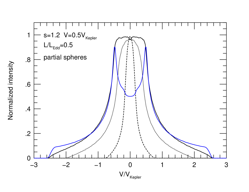
Figure 4.— Same initial conditions as in Fig. 2 for $\Gamma=0.5$. The various profiles represent motion in different spherically shaped atmospheres. The narrowest profile (dashed line) represents a sphere where clouds occupy only the section between -0.3 and +0.3 radians relative to the mid-plane (which is perpendicular to the line of sight). The other cases are for wider coverage with clouds between -0.9 and +0.9 rad (dotted line) and -1.5 to +1.5 rad (solid line). The double peak profile illustrates the case of two polar caps where the clouds occupy a sphere whose mid-section, between -1.2 and +1.2 rad, has been removed.

3.2. Applications to spectroscopic observations of AGNs

The examples discussed above were normalized to give a typical $r_{BLR}$(H$\beta$) for AGNs with $M_{\rm BH}$=$10^{8}$$M_{\odot}$ and $\Gamma=0.1$. However, the computed line profiles cannot be directly compared with the observations of such sources for several reasons. First, we only consider a situation involving one type of clouds and neglect the possibility of different populations under different physical conditions in the same source. This applies to the distributions of both ${N_{\rm col}}$ and $U(r)$. For example, eqn. 1 and the constants given in §1 suggest that, in general, $r_{BLR}(H_{\beta})$/$r_{BLR}(Civ\lambda 1549)\simeq 3$. The question is whether cloud distributions like those considered in Table 1 can reproduce this ratio. Second, we did not take into account changes in $\alpha(r)$, the fraction of $L_{bol}$ which is absorbed by clouds at various distances. This can be an important factor close to the BH where clouds become partly transparent. In this case, much of the Lyman continuum radiation is not absorbed and radiation pressure force is reduced. It can also affect medium to large column density clouds at large distances where $\alpha(r)$ approaches unity. For example, assuming $\alpha(r)=0.75$ instead of $\alpha(r)=0.5$ in the calculations of Table 1 results in a limiting value of $\Gamma$ which is about 0.4 compared with $\Gamma=0.735$ listed in the table.

To illustrate these effects, and to provide more realistic line profiles, we computed two grids of photoionization models for a range of column density and ionization parameter using the code ION (Netzer 2006). The first grid supplies calculated line intensities for H$\beta$ and C iv $\lambda 1549$  over a large range in $U(r)$. Given $r$ from the cloud motion simulation, we use the grid to compute $j(r)$ and thus a more realistic $\epsilon(r)$. The second grid supplies the absorbed fraction, $\alpha(r)$, as a function of $U(r)$ and ${N_{\rm col}}$. Fig. 5 shows part of the $\alpha(r)$ grid to illustrate the expected range in this parameter. We have not included the changes in gas density since they do not play a major role over the range of conditions considered here. We have also not considered anisotropy of the line emission which is bound to have an effect on the FWHM of some lines. Such modifications will be included in a forthcoming paper that is intended to present a comparison with observed line profiles.

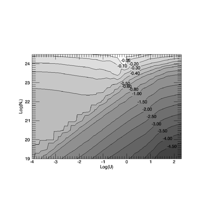
Figure 5.— Part of the $\alpha(r)$ grid (fraction of the total continuum flux absorbed by the clouds) used in the present calculations. Numbers along the contour lines are $log\,\,\alpha$.

We tested a large number of single-zone models using the above grids of $U(r)$ and $\alpha(r)$. The models cover a large range in angular momentum and BLR geometries. We have specifically investigated three cases of different eccentricity, defined by three values of $v_{0}(r_{0})$, 0.25, 0.5 and 0.75. These were calculated with different $\Gamma$ and $r_{23}$. In general, it is easy to reproduce the observed I(C iv $\lambda 1549$)/I(H$\beta$) but difficult to account, at the same time, for the emissivity weighted radii of the two lines (eqn. 1) and the line width ratio. For example, the best case of the three, with $v_{0}(r_{0})=0.25$, gives I(C iv $\lambda 1549$)/I(H$\beta$)=4.4, $<r>$(C iv $\lambda 1549$)/$<r>$(H$\beta$)=0.67 and FWHM(C iv $\lambda 1549$)/FWHM(H$\beta$)=1.43. The conclusion is that, within the range of parameters assumed here, there is no obvious way to explain all those properties when keeping with the idea of a single column density distribution (i.e. a single $r_{23}$).

We also tested a case of $M_{\rm BH}$$=10^{8}$$M_{\odot}$, $\Gamma=0.1$ and two distinct cloud populations in inner and outer zones with some overlap between the two. In this case, the initial conditions for the two populations are decoupled from each other but the changes in density, column density and ionization parameter follow the same pattern with the same $s=1.2$ density law. The FWHM of both emission lines were calculated under the assumption of a thick central spherical sector with clouds occupying a region of $\pm\pi/4$ radians relative to the central plane. The inner zone clouds have $r_{0}=5\times 10^{16}$ cm and $U(r_{0})=10^{-1}$ and the outer-zone clouds $r_{0}=3\times 10^{17}$ cm and $U(r_{0})=10^{-2.5}$. The starting velocity in both zones is $v_{0}=0.5$ at the appropriate $r_{0}$. In both zones $r_{23}=3r_{0}$. We followed the cloud motion and calculated, in each zone, the line intensity ratio, I(C iv $\lambda 1549$)/I(H$\beta$), the line FWHMs, and the emissivity weighted radii. These numbers are listed in Table 2 where we also show the properties of the combined spectrum which is calculated under the assumption of equal contributions to H$\beta$ from both zones. The emissivity weighted radii for the two zones are given in units of the RM-radii of the two lines (eqn. 1). This very simple two-zone model gives results that are in good agreement with the observations of many low-to-intermediate luminosity AGNs. Fig. 6 is a graphical summary of these results. The left and central panels show H$\beta$ and C iv $\lambda 1549$ profiles for the inner and outer zones, again assuming isotropic line emission, and the right panel shows the combined two-zone profiles.

Table 2Properties of the two-zone model with $v_{0}(r_{0})=0.5$.

Zone	FWHM(H$\beta$)	FWHM($Civ$)	$\frac{r({\rm H}\beta)}{r(RM,{\rm H}\beta)}$	$\frac{r(Civ)}{r(RM,Civ)}$	$\frac{I(Civ)}{I({\rm H}\beta)}$
	(km s-1)	(km s-1)
Inner	3160	3450	0.32	0.88	9.55
Outer	1390	2580	1.64	3.2	1.45
Combined	2060	3390	0.98	1.1	5.5

Figure 6.— Calculated H$\beta$ (solid line) and C iv $\lambda 1549$ (dashed line) profiles for a two zone model. Left: line profile for the inner zone. Middle: line profiles for the outer zone. Right: The combined line profile. For FWHMs and general normalization see Table 2.

In conclusion, the simple single zone models explored here cannot reproduce all the observed properties: line intensity ratio, mean emissivity radii and FWHM ratio. The main reason is that the starting conditions fix the cloud orbit, and hence the line emissivity and FWHM. Simple two-zone models like the ones presented here can account for most observed properties of the H$\beta$ and C iv $\lambda 1549$ lines. In particular, they can account for the mean line ratio, the mean emissivity weighted radii and the mean relative FWHM of the H$\beta$ and C iv $\lambda 1549$ lines measured in various RM samples. Obviously, such simple models do not intend to explain all the observed line profile properties that can differ from one object to the next and contain additional components (see some obvious examples for complex C iv $\lambda 1549$ profiles in Richards et al. 2002 and Sulentic et al. 2007). Fitting those is deferred to a forthcoming paper.

4. Discussion

4.1. General considerations

The above calculations allow us to investigate the intensity, the width and the shape of the broad emission lines and to evaluate various methods used to estimate $M_{\rm BH}$. We defer the discussion of specific observed line profiles to a future paper.

Assume a system of clouds with a given total amount of gas and a large range of column densities. Such a system will eventually break into three: virialized clouds, non-virialized bound clouds and escaping clouds. The third group will not contribute significantly to the observed line emission for more than several dynamical times. The relative contribution of the first and second groups to the line emission depend on the cloud mass distribution. A sudden increase in $L_{bol}$ will increase the importance of radiation pressure and will remove more gas from the system. A decrease in $L_{bol}$ will drive the system closer to virial equilibrium. A new gas supply, e.g. from a disk-wind, will produce bound as well as unbound clouds. All aspects of this general scenario must be considered when evaluating the observed line profiles and the various methods developed to use them in estimating $M_{\rm BH}$.

A major objective of the present paper is to evaluate the accuracy and the normalization of various $M_{\rm BH}$ estimators in type-I AGNs. The results presented in Tables 1 & 2 suggest the following:

1. Every AGN is likely to contain a large number of clouds with a large range in ${N_{\rm col}}$. This can be the result of a broad cloud mass distribution and/or due to cloud motion in a radial-pressure dependent environment with a positive value of $s$. A given $\Gamma$ results in a lower limit on ${N_{\rm col}}$ at a given location for a given orbit eccentricity. Under such conditions, there are always some clouds, e.g. those that are very close to the BH, for which radiation pressure is negligible. For others, radiation pressure can be very important.

2. For a small enough ${N_{\rm col}}$, the effective $r_{BLR}$ depends on both $\Gamma$ and ${N_{\rm col}}$. Under these conditions, the BH mass itself is an important factor in determining $r_{BLR}$. To illustrate this, consider two AGNs with identical SED, $L_{bol}$, BLR geometry, ${N_{\rm col}}$ distribution and inclination to the line of sight. The effective $r_{BLR}$ in the two is the same provided they harbor identical BHs. Different $r_{BLR}$ will be measured if the two BHs have different masses despite of the fact that $L_{bol}$ is the same in both. This is the result of the larger $\Gamma$ in the smaller BH AGN. The effect may not be recognized in a large sample of sources and can, in fact, be attributed to a large intrinsic scatter in the $L_{bol}-r_{BLR}$ relationship. Any derived $L_{bol}-r_{BLR}$ relationship will depend on the properties of the sources in the chosen RM sample, in particular on the distribution of $\Gamma$.

3. Assuming a range in ${N_{\rm col}}$ in every AGN, the M08 suggestion to include a luminosity dependent term in the calculation of $M_{\rm BH}$ (eqn. 3) is not in accord with our calculation that indicate that $r_{BLR}$ and FWHM depend on $L/M$ and not on $L$.

The multi-year RM campaign of NGC 5548 is the best example to test some of these ideas in a specific source. The campaign has been described and analyzed in numerous papers and the ones most relevant to the present study are Peterson et al. (1999) and Gilbert and Peterson (2003).

Fig. 7 shows the variations in $L_{5100}$ and time lag (in this case the centroid of the CCF) in NGC 5548. Each point represents a full observing season which is typically $\sim 300$ days long. The data are taken from the recent compilation of Bentz et al. (2009) which provides the best galaxy subtracted flux at 5100Å. The uncertainty on $L_{5100}$ is basically the range of this quantity over the observing season. This is of the same order as the variation from one season to the next. As clearly seen from the diagram, $r_{BLR}$(H$\beta$) lags the continuum in such a way that more luminous phases are associated with longer lags. This has been noted in earlier publications, e.g. Gilbert and Peterson (2003). Fig. 8 shows t(lag) vs. $L_{5100}$ for the same data set. While the uncertainties are large, some correlation, with a slope of 0.5-1, is evident. An earlier version of the diagram, with fewer points, is shown in Peterson et al. (1999).

Figure 7.— Changes in continuum luminosity ($L_{5100}$) and time lag for NGC 5548 (data from Bentz et al. 2009). Error bars on $L_{5100}$ were omitted for clarity.

Figure 8.— The correlation of $L_{5100}$ vs. t(lag) for NGC 5548. Data as in fig. 7. The dashed line has a slope of 0.5.

For NGC 5548, $M_{\rm BH}$$\simeq 10^{8}$ $M_{\odot}$ and $r_{BLR}$(H$\beta$)$\simeq 20$ l.d.. Thus, the dynamical time is of order 6 years and the time it takes to change $r_{BLR}$ by 50% (e.g. Table 1) is approximately 3 years. This seems to be compatible with the changes in $L_{5100}$ and t(lag) in fig. 7, thus some adjustment of $r_{BLR}$(H$\beta$) due to the effects discussed in this work are possible. The measured $L_{5100}$, with a bolometric correction factor of about 10, indicates a mean $\Gamma$ of about 0.02. The bottom part of Table 1 provides approximate parameters for such a case. Any successful model of NGC 5548 should account for the behavior shown in Fig. 7, as well as for the observed FWHMs and luminosities of both H$\beta$ and C iv $\lambda 1549$. While the full investigation is deferred to a future paper, we consider here the predicted lags for $\Gamma$ =0.005, 0.01, 0.02 assuming a BH mass of 10⁸ M_⊙ and two families of clouds: one with $r_{23}=10r_{0}$ and $v_{0}=0.5$, and one with $r_{23}=0.093r_{0}$ and $v_{0}=0.25$. The second assumed family of clouds results in pseudo-orbits of higher eccentricity that, as explained earlier, are more strongly affected by radiation pressure. In both cases, the predicted lags for $\Gamma=0.02$ are consistent with the observed values ($\log t$(lag) $\approx$ 1.34 at $\log L_{5100}\approx 43.48$). However, the calculated slope of $\log t$(lag) vs. $L_{5100}$ is flatter than observed.

As argued earlier, a single family of BLR clouds cannot provide a full explanation to the observed spectrum of many AGNs. This must applied to NGC 5548 (to appreciate the complexity of this case see the various components considered by Kaspi and Netzer (1999) to explain only the variable line intensities). The simple examples considered here suggests that dynamical scaling of the BLR in NGC 5548, due to radiation pressure force, is an additional, physically-motivated mechanism that must be added to any cloud model when attempting to explain the observed variations in $t$(lag).

4.2. Evaluation of present $M_{\rm BH}$ estimators

Current BH mass estimates utilize RM-based measurements of $r_{BLR}$, measured FWHMs (or an equivalent velocity estimator) of certain broad emission lines, and eqn. 2. The normalization constant $f$ is obtained by a comparing $M_{\rm BH}$ obtained in this way with the mass obtained from the $M-{\sigma*}$ method. Having examined a large range of cloud orbits and line profiles under various conditions, and the corresponding values of the effective $r_{BLR}$, we are now in a position to evaluate the merits of this method.

We consider three general possibilities. The first is the case where all AGNs contain BLR clouds with a wide column density distribution. A randomly chosen object will have in its BLR some clouds that are affected by radiation pressure force and others that are not. This is the case for any $\Gamma$. The cloud dynamics and the observed line profiles reflect the (unknown) column density distribution. Our calculations suggest that an RM sample drawn randomly from such an AGN population can be safely used to determine the best value of $f$ by comparing the derived $M_{\rm BH}$  with the $M-{\sigma*}$ method. This is justified by the fact that $M_{BH}\propto<r>FWHM^{2}$ even if radiation pressure force is important (see Table 1). The observed FWHMs are, indeed, smaller than the ones that would have been observed if all clouds had extremely large column densities. This, however, has no practical implication since the column densities are not known and $f$ is simply a normalization factor that serves to bring two completely different methods of estimating $M_{\rm BH}$ into agreement. Mass estimates obtained in this ways are reliable provided the properties of the RM sample represent well the population properties.

The second case reflects a situation where the cloud column density distribution is, again, very broad but part of the population is under-represented in the RM sample. For example, the RM sample may contain mostly sources with $\Gamma\sim 0.1$ while the overall distribution of $\Gamma$ is much wider. In this case, the normalization factor $f$ will reflect only the properties of the measured sources and its use will provide poor mass estimates for cases with much larger or much smaller accretion rates. This may well be the case in the RM sample which is most commonly used (Kaspi et al. 2000; Bentz et al, 2009) that contains only very few AGNs with $\Gamma>0.3$. The numbers in Table 1 enable us to evaluate the resulting deviations in the estimated $M_{\rm BH}$. For example, if we use the first part of the table and assume a source with a certain $L_{bol}$ and $\Gamma=0.1$, we find that the mass of a similar $L_{bol}$ source with $\Gamma=0.7$ will be under-estimated by a factor of 1.11/0.75.

Regarding the second case, it is important to note that under-estimates and over-estimates of $M_{\rm BH}$ are equally likely. Consider again an RM sample where, for most sources, $\Gamma=0.1$. This results in a certain value of $f$ which takes into account the effect of radiation pressure force in some of these sources (see bottom part of Table 1). Assume a second, randomly selected AGN sample with a similar BH mass distribution but a typical $\Gamma$ which is much smaller than 0.1. Most measured FWHMs in this sample are broader than those in the RM sample because radiation pressure force is not as effective in reducing the cloud velocity. Using the value of $f$ derived for the RM sample will result in over estimating $M_{\rm BH}$ in the second sample. The lower part of Table 1 gives some idea about the magnitude of this effect, e.g. an over estimate by a factor of 1.01/0.76.

The third case is similar to the first one except that large luminosity variations, on time scales that are not too different from the BLR dynamical time, are occurring in most sources, including those selected for RM monitoring. Table 1 shows that, like the first case, the deduced $f$ represents well the population because $<r>$ follows the variations in $L_{bol}$. The mean $M_{\rm BH}$ in such a sample is recovered albeit with a larger uncertainty.

4.3. Alternative $M_{\rm BH}$ estimators

Given the above considerations, we now investigate an alternative method to calculate $M_{\rm BH}$. The method takes into account the effect of radiation pressure force on the cloud motion and the results will be compared to those obtained by the old method (eqn. 2) and by the M08 method.

Our new calculations indicate that the emissivity weighted $r_{BLR}$ depends both on the (large) range in $L$ across the entire AGN population, as well as on short time scale changes in $r_{BLR}$ in individual sources. The first of those depends roughly on $L^{1/2}$ and is a manifestation of the observational fact that the ionization parameter, $U(r)$, and the spectral energy distribution (SED), are not changing much with source luminosity. The second reflects changes in the BLR structure due to the reaction of various column density clouds to the (changing) radiation pressure force. This depends on both $L_{bol}$ and $M_{\rm BH}$. This is seen for example in eqn. 12 for the critical radius where clouds can escape the system and also in the calculations of Table 1. It is therefore reasonable to assume that $r_{BLR}$ is given by an expression of the form,

$$r_{BLR}=a_{1}L^{\gamma}+a_{2}(L/M)^{\delta}\,\,,$$ (17)

where $a_{1}$ and $a_{2}$ are constants and $L$ is a measure of the source luminosity, e.g. $L_{5100}$ if $r_{BLR}$=$r_{BLR}$(H$\beta$). Obviously, the above approximation is not unique and one can assume other dependences that are consistent with the line profile calculations, e.g. a dependence of FWHM on $L/M$.

The idea of introducing a second, luminosity dependent term into the calculation of $M_{\rm BH}$ is not new. In particular, M08 suggested an expression for $M_{\rm BH}$ which depends on both $L^{1/2}$ and $L/N_{col}$ (eqn. 3). Assuming all AGNs obey the same relationship, and ${N_{\rm col}}$ is the same in all, the M08 expression leads to extremely large values of $M_{\rm BH}$ for the most luminous AGNs. The reason is the linear dependence of $M_{\rm BH}$ on $L$ at very high luminosities combined with the calibration of the relationship at small $L$, typical of the $M-{\sigma*}$ sample of Onken et al. (2004). The additional consequence of this approach is an upper limit of $\Gamma\sim 0.1$ in many high luminosity, large BH mass sources. In their later work, M09 considered the possibility that ${N_{\rm col}}$ can differ from one source to another but is still constant for all clouds in a given BLR. This would result in smaller $M_{\rm BH}$ and larger $\Gamma$ in some high luminosity sources since in some BLRs, ${N_{\rm col}}$ can exceed $10^{23}$ cm^-2 by a large factor thus reducing the importance of radiation pressure force.

The limitation of the M08 mass estimate is the detachment of $L$ from $M_{\rm BH}$. As shown here, this is not the case in more realistic BLRs, especially those where the masses of the clouds are conserved. In such cases, the location of the outer clouds that still contribute to the line profiles depends on $L/M$ and the 3D-velocities of the marginally bound clouds are such that the product $r_{BLR}$$FWHM^{2}$ is not very different from what is found in pure gravity dominated systems. Moreover, for pressure confined clouds, the dependence on ${N_{\rm col}}$ is likely to be different in different parts of the BLR. Thus, we are looking for an expression that will reflect, properly, all these effects and will allow for the possibility of a range of column densities in every source. We also want to avoid biasing in the derivation of $M_{\rm BH}$ in the limits of very large or very small $L$ and to retain the experimental results that $r_{BLR}\propto L^{\gamma}$ with $\gamma=0.6\pm 0.1$.

All the above can be achieved by assuming that $r_{BLR}$ is given by eqn. 17 and requiring that $M_{BH}\propto r_{BLR}FWHM^{2}$. For the sake of simplicity, we assume $\gamma=0.5$ and $\delta=1$ and substitute eqn. 17 into the mass expression. This leads to a simple quadratic equation in $M_{\rm BH}$ with the following solution,

$$M_{BH}=\frac{1}{2}a_{1}L^{1/2}FWHM^{2}\left[1+\sqrt{(}1+\frac{4a_{2}}{a_{1}^{2}FWHM^{2}})\right]\,\,,$$ (18)

where $a_{1}$ and $a_{2}$ are the same ones used in eqn. 17 except for a common multiplicative constant which depends on the units of $r_{BLR}$, $L_{5100}$ and $M_{\rm BH}$. For example, using the measure parameters for the H$\beta$ line, $L=$$L_{5100}$, FWHM=FWHM(H$\beta$), then the constant multiplying $a_{1}$ and $a_{2}$ in eqn. 17 is 10^16.123 when $M_{\rm BH}$ is measured in $M_{\odot}$, $L_{5100}$ in units of $10^{44}$ ergs s^-1 and $r_{BLR}$ in cm.

We used eqn. 18 and the Woo et al. (2010) sample to find $a_{1}$ and $a_{2}$ for 29 AGNs with measured $\sigma*$. The list is an extension of the one used by Onken et al. (2004) that contains only 16 sources. We have supplemented the data in Woo et al. by data from Bentz et al. (2009) on $r_{BLR}$ and $L_{5100}$ where this information was missing. First, we performed a $\chi^{2}$ analysis on $M_{\rm BH}$(RM) vs. $M-{\sigma*}$ using the parameters recommended by Gültekin et al. (2009). This gave $f=1.0$ which is consistent with the values found by Onken et al. (2004) and Woo et al. (2010)

Next we carried out a $\chi^{2}$ minimization to solve for $a_{1}$ and $a_{2}$ in eqn. 18. Since the minimization involves the error estimate on $L_{5100}$, and since this error is not very well defined given the combination of observational uncertainly and the intrinsic scatter in $L_{5100}$ over several long RM campaigns, we decided to adopt a uniform value of $\Delta L_{5100}/L_{5100}=0.3$. We also assume a minimum of 0.1 to $\Delta(\sigma*)/\sigma*$ and a minimum of 0.05 on $\Delta(FWHM)/FWHM$. Our results depend slightly on these assumptions.

The best values obtained in this procedure are $a_{1}=4.1$, $a_{2}=7.1\times 10^{7}$ and $\chi^{2}/{\nu}=1.73$. Extensive tests show that the $\chi^{2}$ changes very little if $a_{1}$ or $a_{2}$ are changing by up to 10%. This is the result of some degeneracy between $a_{1}$ and $a_{2}$ (see eqn. 18). The average deviation between the new mass estimates and those obtained by the $M-\sigma*$ method is 0.31 dex. There is a weak dependence of the deviation on the line width (larger deviation for larger FWHM(H$\beta$)) which is marginal given the small number of sources in the sample. The corresponding number for the deviation of masses obtained directly from the RM measurements and the above value of $f$ is 0.36 dex. Thus the new method is, indeed, superior in this respect. Obviously it is not surprising to find such an improvement when adding a new free parameter to the model.

To compare the various mass estimates more thoroughly, we calculated $M_{\rm BH}$ in three different ways: the old method (eqn. 2) with $f=1.0$, the M08 method (eqn. 3) with $f_{1}=0.56$ and $f_{g}=10^{7.7}$ (as in M08), and the new method (eqn. 18) with the above $a_{1}$ and $a_{2}$. For the M08 method, we followed the M09 recommendation and assumed a log normal distribution of ${N_{\rm col}}$ with a mean of $10^{23}$ cm^-2 and a large standard deviation of 0.5 dex. We also calculated $r_{BLR}$ in the old (eqn. 1) and new (eqn. 17) ways.

Fig. 9 compares two mass ratios, $M_{\rm BH}$(new)/$M_{\rm BH}$(old) (red points) and $M_{\rm BH}$(new)/$M_{\rm BH}$(M08) (black points), in a large simulated AGN sample. The sample covers, uniformly, the luminosity range $L_{5100}$=$10^{43}-10^{47}$ ergs s^-1 and the simulations assume a Gaussian, luminosity independent distribution of FWHM(H$\beta$) with a mean of 4,500 km s^-1 and a variance of 1,500 km s^-1. The diagram shows that the new and old estimates are similar at all $L_{bol}$ but $M_{\rm BH}$(M08) deviates from both, by a large factor, at both low and high luminosities. Moreover, the slight deviation between the new and old methods at the very high luminosity end, by up to about 0.2 dex in $M_{\rm BH}$, is most likely due to the fact that the procedure used to obtain $a_{1}$ and $a_{2}$ is based on a sample of 29 mostly low-to-intermediate luminosity AGNs while the simulations reach a much larger value of $L_{bol}$. A comparison of the estimated $r_{BLR}$ (eq. 1 and 17) leads to similar conclusions.

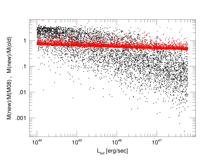
Figure 9.— Comparison of the various methods for calculating $M_{\rm BH}$. The ratio of the new-to-old (red) and new-to-M08 (black) methods are shown as a function of $L_{bol}$ for the simulated sample described in the text. Note the good agreement between the old and the new methods and the large deviation from the method described in M08 for very large and very small values of $L_{bol}$.

We also made a similar test on the Netzer and Trakhtenbrot (2007) sample using all three methods. The luminosity range in this case is smaller but the FWHM(H$\beta$) distribution more typical of observed AGNs. The results (not shown here) are very similar to those of the simulated sample.

In conclusion, the new method for estimating $M_{\rm BH}$ gives results that do not deviate much from the old method which is based on a single constant $f$. This is true at both high and low luminosities and over a large range in FWHM. Obviously, the range of parameters tested here ($s$, orbit eccentricity, several types of cloud distributions, etc.) is rather limited and more extensive modeling is required to confirm these results. However, it is our opinion that the main limitation of the $M_{\rm BH}$ determination methods remains observational and is related to the fact that the present AGN $M-{\sigma*}$ sample is small (29 sources) and cannot possibly represent the entire range of properties, mostly $\Gamma$, observed in AGNs.

5. Conclusions

We have investigated the motion of BLR clouds with time-independent mass under a range of conditions defined by a radial-dependent confining pressure. These conditions enforce a range of ${N_{\rm col}}$ in every BLR, even if the intrinsic mass distribution of the cloud is narrow. We calculated cloud orbits under a central potential that includes a radiation pressure term. The orbits were then combined to predict emission line profiles in several simple situations. We only considered uniformly emitted emission lines and the preliminary comparison with with actual observations used realistic emissivity and column density distributions but was limited to the H$\beta$ and C iv $\lambda 1549$ lines and at most two different cloud distributions. We found significant changes in cloud locations and velocities for those cases where the column densities are small enough to allow a significant contribution due to radiation pressure. This can be important in both high and low $\Gamma$ sources. However, while cloud orbits are strongly influenced by the radiation pressure force, there is a relatively small change in the mean $r_{BLR}$$FWHM^{2}$ and hence no large underestimation or overestimation of $M_{\rm BH}$. We illustrate this behavior in several cases but note that other cloud distributions, with different mass, location and velocity distributions, may lead to somewhat different conclusions. We used the new results to suggest a novel method for calculating $r_{BLR}$ and $M_{\rm BH}$ by applying two new constants that were calculated by a comparison of the H$\beta$ and $L_{5100}$ observations and the $M-\sigma*$ AGN sample of Woo et al. (2010). We applied the method to several large observed and simulated AGN samples and demonstrated good agreement between the new and the old, pure gravity based methods. The comparison with the M08 methods shows large deviations in the estimates of $M_{\rm BH}$.

References

- Baldwin et al. (1995) Baldwin, J. A, et al. 1995, ApJ, 455, L119
- Bentz et al. (2009) Bentz, M., Peterson, B.M., Netzer, H., Pogge, R.W., & Vestergaard, M, 2009 ApJ, 697, 160
- Bottorff et al. (1997) Bottorff, M., Korista, K.T., Shlosman, I., & Blandford, R.D. 1997, ApJ, 479, 200
- Bottorff (2000) Bottorff, M., & Ferland, G.J 2000 MNRAS, 316, 103
- Chiang & Murray (1996) Chiang, J., & Murray, N. 1996, ApJ, 466, 704
- Collin et al. (2006) Collin, S., Kawaguchi, T., Peterson, B. M., Vestergaard, M. 2006, A&A, 456, 75
- Everett (2003) Everett, J. E. 2003, Ph. D. Thesis, The University of Chicago
- Ferland (2009) Ferland, G.J, Hu, Chen, Wang, Jian-Min, Baldwin, J.A, Porter, R.L, vanHoof, P., Peter, A.M, & Williams, R.J.R, 2009, ApJ, 707, L82
- Korista et al. (1995) Korista, K.T., et al. 1995, ApJS, 97, 285
- Gilbert & Peterson (2003) Gilbert, K. M., & Peterson B. M. 2003, ApJ, 578, 123
- Gültekin et al. (2009) Gültekin, K., et al. 2009, ApJ, 698, 198.
- Jarvis & McLure (2006) Jarvis, M. J., & McLure, R. J. 2006, MNRAS 369, 182
- Kaspi & Netzer (1999) Kaspi, S., & Netzer, H. 1999, ApJ, 524, 71
- Kaspi et al. (2000) Kaspi, S., Smith, P. S., Netzer, H., Maoz, D., Jannuzi, B. T., & Giveon, U. 2000, ApJ, 533, 631
- Kaspi et al. (2005) Kaspi, S., Maoz, D., Netzer, H., Peterson, B. M., Vestergaard, M., & Jannuzi, B. T. 2005, ApJ, 629, 61
- Kaspi et al. (2007) Kaspi, S., et al. 2007, ApJ, 659, 997
- Korista & Goad (2004) Korista, K. T., & Goad, M. R. 2004, ApJ, 606, 749
- Maiolino et al. (2010) Maiolino, R., et al. 2010, A&A, 517, A47
- Marconi et al. (2008) Marconi, A., Axon, D. J., Maiolino, R., Nagao, T., Pastorini, G., Pietrini, P., Robinson, A., & Torricelli, G. 2008a, ApJ, 678, 693 (M08)
- Marconi et al. (2009) Marconi, A., Axon, D. J., Maiolino, R., Nagao, T., Pietrini, P., Risaliti, G., Robinson, A., & Torricelli, G. 2009, ApJ, 698, L103 (M09)
- Marziani et al. (1996) Marziani, P., Sulentic , J. W., Dultzin-Hacyan, D., Calvani, M., Moles, M. 1996, ApJS, 104, 47
- Murray & Chiang (1997) Murray, N., & Chiang, J. 1997, ApJ, 474, 91
- Netzer (1990) Netzer, H. 1990, 20. Saas-Fee Advanced Course of the Swiss Society for Astrophysics and Astronomy: Active galactic nuclei, Berlin, Springer, p. 57 - 160
- Netzer (2009) Netzer, H. 2009, ApJ, 695, 793
- Netzer & Trakhtenbrot (2007) Netzer, H., & Trakhtenbrot, B. 2007, ApJ, 654, 754
- Onken et al. (2004) Onken, C. A., Ferrarese, L., Merritt, D., Peterson, B. M., Pogge, R. W., Vestergaard, M., & Wandel, A. 2004, ApJ, 615, 645
- Peterson et al. (1999) Peterson, B. M., et al., 1999, ApJ, 510, 668
- Proga et al. (2000) Proga, D., Stone, J. M., Kallman, T. R. 2000, ApJ, 543, 686
- Rees (1989) Rees, M., Netzer, H., & Ferland, G. J., 1989, ApJ, 347, 640
- Richards et al. (2002) Richards, G. T. and Vanden Berk, D. E. and Reichard, T. A. and Hall, P. B. and Schneider, D. P. and SubbaRao, M. and Thakar, A. R. and York, D. G. 2002, AJ, 124, 1
- Risaliti et al. (2010) Risaliti, G., Elvis, M., Bianchi, S., Matt, G. 2010, MNRAS, in press, eprint arXiv:1005.3052
- Smith et al. (2004) Smith, J. E., Robinson, A., Alexander, D. M., Young, S., Axon, D. J., Corbett, E. A. 2004, MNRAS, 350, 140
- Sulentic et al. (2007) Sulentic, J., et al. 2007, ApJ, 666, 757
- Tremaine et al. (2002) Tremaine, S., et al. 2002, ApJ, 574, 740
- Vestergaard & Peterson (2006) Vestergaard, M., & Peterson, B. M. 2006, ApJ, 641, 689
- Vestergaard et al. (2000) Vestergaard, M., Wilkes, B. J., Barthel P. D. 2000, ApJ, 538, L103
- Woo et al. (2010) Woo, J.-H., et al. 2010, ApJ, 716, 269
- Young et al. (2007) Young, S., Axon, D. J., Robinson, A., Hough, J. H., Smith, J. E. 2007, Nature, 450, 74