Introduction to flavor physics

Abstract

This set of lectures covers the very basics of flavor physics and are aimed to be an entry point to the subject. A lot of problems are provided in the hope of making the manuscript a self study guide.

I Welcome statement

My plan for these lectures is to introduce you to the very basics of flavor physics. Hopefully, after the lectures you will have enough knowledge and more importantly, enough curiosity, that you will go on and learn more about the subject.

These are lecture notes and are not meant to be a review. I try to present the basic ideas, hoping to give a clear picture of the physics. Thus, many details are omitted, implicit assumptions are made, and no references are given. Yet details are important: after you go over the current lecture notes once or twice, I hope you will feel the need for more. Then it will be the time to turn to the many reviews Gedalia:2010rj ; Isidori:2010gz ; Buras:2009if ; Nierste:2009wg ; Artuso:2009jw ; Nir:2007xn ; Hocker:2006xb ; Neubert:2005mu ; Nir:2005js ; Buras:2005xt ; Ligeti:2003fi and books Bigi:2000yz ; Branco:1999fs on the subject.

I have tried to include many homework problems for the reader to solve, much more than what I gave in the actual lectures. If you would like to learn the material, I think that the provided problems are the way to start. They force you to fully understand the issues and apply your knowledge to new situations. The problems are given at the end of each section. The questions can be challenging and may take a lot of time. Do not give up after a few minutes!

II The standard model: a reminder

I assume that you have basic knowledge of Quantum Field Theory (QFT) and that you are familiar with the Standard Model (SM). Nevertheless, I start with a brief review of the SM, not only to remind you, but also since I like to present things in a way that may be different from the way you got to know the SM.

II.1 The basic of model building

In high energy physics, we ask a very simple question: What are the fundamental laws of Nature? We know that QFT is an adequate tool to describe Nature, at least at energies we have probed so far. Thus the question can be stated in a very compact form as: what is the Lagrangian of nature? The most compact form of the question is

$${\cal L}=?$$ (1)

In order to answer this question we need to provide some axioms or “rules.” Our rules are that we “build” the Lagrangian by providing the following three ingredients:

1. The gauge symmetry of the Lagrangian;

2. The representations of fermions and scalars under the symmetry;

3. The pattern of spontaneous symmetry breaking.

Once these ingredients are provided, we write the most general renormalizable Lagrangian that is invariant under these symmetries and provide the required spontaneous symmetry breaking (SSB).

Few remarks are in order about these starting points.

1. We also impose Poincare invariance. In a way, this can be identified as the gauge symmetry of gravity, and thus can be though of part of the first postulate.

2. As we already mentioned, we assume QFT. In particular, quantum mechanics is also an axiom.

3. We do not impose global symmetries. They are accidental, that is, they are there only because we do not allow for non renormalizable terms.

4. The basic fermion fields are two component Weyl spinors. The basic scalar fields are complex. The vector fields are introduced to the model in order to preserve the gauge symmetry.

5. Any given model has a finite number of parameters. These parameters need to be measured before the model can be tested. That is, when we provide a model, we cannot yet make predictions. Only after an initial set of measurements are done can we make predictions.

As an example we consider the SM. It is a nice example, mainly because it describes Nature, and also because the tools we use to construct the SM are also those we use when constructing its possible extensions. The SM is defined as follows:

1. The gauge symmetry is

   $$G_{\rm SM}=SU(3)_{\rm C}\times SU(2)_{\rm L}\times U(1)_{\rm Y}.$$ (2)

2. There are three fermion generations, each consisting of five representations of $G_{\rm SM}$:

   $$Q^{I}_{Li}(3,2)_{+1/6},\quad U^{I}_{Ri}(3,1)_{+2/3},\quad D^{I}_{Ri}(3,1)_{-1/3},\quad L^{I}_{Li}(1,2)_{-1/2},\quad E^{I}_{Ri}(1,1)_{-1}.$$ (3)

   Our notations mean that, for example, left-handed quarks, $Q_{L}^{I}$, are triplets of $SU(3)_{\rm C}$, doublets of $SU(2)_{\rm L}$ and carry hypercharge $Y=+1/6$. The super-index $I$ denotes gauge interaction eigenstates. The sub-index $i=1,2,3$ is the flavor (or generation) index. There is a single scalar representation,

   $$\phi(1,2)_{+1/2}.$$ (4)

3. The scalar $\phi$ assumes a VEV,

   $$\langle\phi\rangle=\pmatrix{0\cr{v/\sqrt{2}}\cr},$$ (5)

   which implies that the gauge group is spontaneously broken,

   $$G_{\rm SM}\to SU(3)_{\rm C}\times U(1)_{\rm EM}.$$ (6)

   This SSB pattern is equivalent to requiring that one parameter in the scalar potential is negative, that is $\mu^{2}<0$, see Eq. (11).

The standard model Lagrangian, ${\cal L}_{\rm SM}$, is the most general renormalizable Lagrangian that is consistent with the gauge symmetry (2) and the particle content (3) and (4). It can be divided to three parts:

$${\cal L}_{\rm SM}={\cal L}_{\rm kinetic}+{\cal L}_{\rm Higgs}+{\cal L}_{\rm Yukawa}.$$ (7)

We will learn how to count parameters later, but for now we just mention that ${\cal L}_{\rm SM}$ has 18 free parameters that we need to determine experimentally. Now we talk a little about each part of ${\cal L}_{\rm SM}$.

For the kinetic terms, in order to maintain gauge invariance, one has to replace the derivative with a covariant derivative:

$$D^{\mu}=\partial^{\mu}+ig_{s}G^{\mu}_{a}L_{a}+igW^{\mu}_{b}T_{b}+ig^{\prime}B^{\mu}Y.$$ (8)

Here $G^{\mu}_{a}$ are the eight gluon fields, $W^{\mu}_{b}$ the three weak interaction bosons and $B^{\mu}$ the single hypercharge boson. The $L_{a}$’s are $SU(3)_{\rm C}$ generators (the $3\times 3$ Gell-Mann matrices ${1\over 2}\lambda_{a}$ for triplets, $0$ for singlets), the $T_{b}$’s are $SU(2)_{\rm L}$ generators (the $2\times 2$ Pauli matrices ${1\over 2}\tau_{b}$ for doublets, $0$ for singlets), and the $Y$’s are the $U(1)_{\rm Y}$ charges. For example, for the left-handed quarks $Q_{L}^{I}$, we have

$${\cal L}_{\rm kinetic}(Q_{L})=i{\overline{Q_{Li}^{I}}}\gamma_{\mu}\left(\partial^{\mu}+{i\over 2}g_{s}G^{\mu}_{a}\lambda_{a}+{i\over 2}gW^{\mu}_{b}\tau_{b}+{i\over 6}g^{\prime}B^{\mu}\right)Q_{Li}^{I},$$ (9)

while for the left-handed leptons $L_{L}^{I}$, we have

$${\cal L}_{\rm kinetic}(L_{L})=i{\overline{L_{Li}^{I}}}\gamma_{\mu}\left(\partial^{\mu}+{i\over 2}gW^{\mu}_{b}\tau_{b}-{i\over 2}g^{\prime}B^{\mu}\right)L_{Li}^{I}.$$ (10)

This part of the Lagrangian has three parameters, $g$, $g^{\prime}$ and $g_{s}$.

The Higgs potential, which describes the scalar self interactions, is given by:

$${\cal L}_{\rm Higgs}=\mu^{2}\phi^{\dagger}\phi-\lambda(\phi^{\dagger}\phi)^{2}.$$ (11)

This part of the Lagrangian involves two parameters, $\lambda$ and $\mu$, or equivalently, the Higgs mass and its VEV. The requirement of vacuum stability tells us that $\lambda>0$. The pattern of spontaneous symmetry breaking, (5), requires $\mu^{2}<0$.

We split the Yukawa part into two, the leptonic and baryonic parts. At the renormalizable level the lepton Yukawa interactions are given by

$$-{\cal L}_{\rm Yukawa}^{\rm leptons}=Y^{e}_{ij}{\overline{L^{I}_{Li}}}\phi E^{I}_{Rj}+{\rm h.c.}.$$ (12)

After the Higgs acquires a VEV, these terms lead to charged lepton masses. Note that the SM predicts massless neutrinos. The Lepton Yukawa terms involve three physical parameters, which are usually chosen to be the three charged lepton masses.

The quark Yukawa interactions are given by

$$-{\cal L}_{\rm Yukawa}^{\rm quarks}=Y^{d}_{ij}{\overline{Q^{I}_{Li}}}\phi D^{I}_{Rj}+Y^{u}_{ij}{\overline{Q^{I}_{Li}}}\tilde{\phi}U^{I}_{Rj}+{\rm h.c.}.$$ (13)

This is the part where quarks masses and flavor arises, and we will spend the rest of the lectures on it. For now, just in order to finish the counting, we mention that the Yukawa interactions for the quarks are described by ten physical parameters. They can be chosen to be the six quark masses and the four parameters of the CKM matrix. We will discuss the CKM matrix at length soon.

The SM has an accidental global symmetry

$$U(1)_{B}\times U(1)_{e}\times U(1)_{\mu}\times U(1)_{\tau}.$$ (14)

where $U(1)_{B}$ is baryon number and the other three $U(1)$s are lepton family lepton numbers. The quarks carry baryon number, while the leptons and the bosons do not. We usually normalize it such that the proton has $B=1$ and thus each quark carries a third unit of baryon number. As for lepton number, in the SM each family carries its own lepton number, $L_{e}$, $L_{\mu}$ and $L_{\tau}$. Total lepton number is a subgroup of this more general symmetry, that is, the sum of all three family lepton numbers. In these lectures we concentrate on the quark sector and therefore we do not elaborate much on the global symmetry of the lepton sector.

II.2 Counting parameters

Before we go on to study the flavor structure of the SM in detail, we explain how to identify the number of physical parameter in any model. The Yukawa interactions of Eq. (13) have many parameters but some are not physical. That is, there is a basis where they are identically zero. Of course, it is important to identify the physical parameters in any model in order to probe and check it.

We start with a very simple example. Consider a hydrogen atom in a uniform magnetic field. Before turning on the magnetic field, the hydrogen atom is invariant under spatial rotations, which are described by the $SO(3)$ group. Furthermore, there is an energy eigenvalue degeneracy of the Hamiltonian: states with different angular momenta have the same energy. This degeneracy is a consequence of the symmetry of the system.

When magnetic field is added to the system, it is conventional to pick a direction for the magnetic field without a loss of generality. Usually, we define the positive $z$ direction to be the direction of the magnetic field. Consider this choice more carefully. A generic uniform magnetic field would be described by three real numbers: the three components of the magnetic field. The magnetic field breaks the $SO(3)$ symmetry of the hydrogen atom system down to an $SO(2)$ symmetry of rotations in the plane perpendicular to the magnetic field. The one generator of the $SO(2)$ symmetry is the only valid symmetry generator now; the remaining two $SO(3)$ generators in the orthogonal planes are broken. These broken symmetry generators allow us to rotate the system such that the magnetic field points in the $z$ direction:

$$O_{xz}O_{yz}(B_{x},B_{y},B_{z})=(0,0,B^{\prime}_{z}),$$ (15)

where $O_{xz}$ and $O_{yz}$ are rotations in the $xz$ and $yz$ planes respectively. The two broken generators were used to rotate away two unphysical parameters, leaving us with one physical parameter, the magnitude of the magnetic field. That is, when turning on the magnetic field, all measurable quantities in the system depend only on one new parameter, rather than the naïve three.

The results described above are more generally applicable. Particularly, they are useful in studying the flavor physics of quantum field theories. Consider a gauge theory with matter content. This theory always has kinetic and gauge terms, which have a certain global symmetry, $G_{f}$, on their own. In adding a potential that respect the imposed gauge symmetries, the global symmetry may be broken down to a smaller symmetry group. In breaking the global symmetry, there is an added freedom to rotate away unphysical parameters, as when a magnetic field is added to the hydrogen atom system.

In order to analyze this process, we define a few quantities. The added potential has coefficients that can be described by $N_{\mathrm{general}}$ parameters in a general basis. The global symmetry of the entire model, $H_{f}$, has fewer generators than $G_{f}$ and we call the difference in the number of generators $N_{\mathrm{broken}}$. Finally, the quantity that we would ultimately like to determine is the number of parameters affecting physical measurements, $N_{\mathrm{phys}}$. These numbers are related by

$$N_{\mathrm{phys}}=N_{\mathrm{general}}-N_{\mathrm{broken}}.$$ (16)

Furthermore, the rule in (16) applies separately for both real parameters (masses and mixing angles) and phases. A general, $n\times n$ complex matrix can be parametrized by $n^{2}$ real parameters and $n^{2}$ phases. Imposing restrictions like Hermiticity or unitarity reduces the number of parameters required to describe the matrix. A Hermitian matrix can be described by $n(n+1)/2$ real parameters and $n(n-1)/2$ phases, while a unitary matrix can be described by $n(n-1)/2$ real parameters and $n(n+1)/2$ phases.

The rule given by (16) can be applied to the standard model. Consider the quark sector of the model. The kinetic term has a global symmetry

$$G_{f}=U(3)_{Q}\times U(3)_{U}\times U(3)_{D}.$$ (17)

A $U(3)$ has 9 generators (3 real and 6 imaginary), so the total number of generators of $G_{f}$ is 27. The Yukawa interactions defined in (13), $Y^{F}$ ($F=u,d$), are $3\times 3$ complex matrices, which contain a total of 36 parameters (18 real parameters and 18 phases) in a general basis. These parameters also break $G_{f}$ down to the baryon number

$$U(3)_{Q}\times U(3)_{U}\times U(3)_{D}\to U(1)_{B}.$$ (18)

While $U(3)^{3}$ has 27 generators, $U(1)_{B}$ has only one and thus $N_{\mathrm{broken}}=26$. This broken symmetry allows us to rotate away a large number of the parameters by moving to a more convenient basis. Using (16), the number of physical parameters should be given by

$$N_{\mathrm{phys}}=36-26=10.$$ (19)

These parameters can be split into real parameters and phases. The three unitary matrices generating the symmetry of the kinetic and gauge terms have a total of 9 real parameters and 18 phases. The symmetry is broken down to a symmetry with only one phase generator. Thus,

$$N^{(r)}_{\mathrm{phys}}=18-9=9,\qquad N^{(i)}_{\mathrm{phys}}=18-17=1.$$ (20)

We interpret this result by saying that of the 9 real parameters, 6 are the fermion masses and three are the CKM matrix mixing angles. The one phase is the CP-violating phase of the CKM mixing matrix.

In your homework you will count the number of parameters for different models.

II.3 The discrete symmetries of the SM

Since we are talking a lot about symmetries it is important to recall the situation with the discrete symmetries, C, P and T. Any local Lorentz invariant QFT conserves CPT, and in particular, this is also the case in the SM. CPT conservation also implies that T violation is equivalent CP violation.

You may wonder why we discuss these symmetries as we are dealing with flavor. It turns out that in Nature, C, P, and CP violation are closely related to flavor physics. There is no reason for this to be the case, but since it is, we study it simultaneously.

In the SM, C and P are “maximally violated.” By that we refer to the fact that both C and P change the chirality of fermion fields. In the SM the left handed and right handed fields have different gauge representations, and thus, independent of the values of the parameters of the model, C and P must be violated in the SM.

The situation with CP is different. The SM can violate CP but it depends on the values of its parameters. It turns out that the parameters of the SM that describe Nature violate CP. The requirement for CP violation is that there is a physical phase in the Lagrangian. In the SM the only place where a complex phase can be physical is in the quark Yukawa interactions. More precisely, in the SM, CP is violated if and only if

$${\cal I}m(\det[Y^{d}Y^{d\dagger},Y^{u}Y^{u\dagger}])\neq 0.$$ (21)

An intuitive explanation of why CP violation is related to complex Yukawa couplings goes as follows. The Hermiticity of the Lagrangian implies that ${\cal L}_{\rm Yukawa}$ has pairs of terms in the form

$$Y_{ij}\overline{\psi_{Li}}\phi\psi_{Rj}+Y_{ij}^{*}\overline{\psi_{Rj}}\phi^{\dagger}\psi_{Li}.$$ (22)

A CP transformation exchanges the above two operators

$$\overline{\psi_{Li}}\phi\psi_{Rj}\ \Leftrightarrow\ \overline{\psi_{Rj}}\phi^{\dagger}\psi_{Li},$$ (23)

but leaves their coefficients, $Y_{ij}$ and $Y_{ij}^{*}$, unchanged. This means that CP is a symmetry of ${\cal L}_{\rm Yukawa}$ if $Y_{ij}=Y_{ij}^{*}$.

In the SM the only source of CP violation are Yukawa interactions. It is easy to see that the kinetic terms are CP conserving. For the SM scalar sector, where there is a single doublet, this part of the Lagrangian is also CP conserving. For extended scalar sectors, such as that of a two Higgs doublet model, ${\cal L}_{\rm Higgs}$ can be CP violating.

II.4 The CKM matrix

We are now equipped with the necessary tools to study the Yukawa interactions. The basic tool we need is that of basis rotations. There are two important bases. One where the masses are diagonal, called the mass basis, and the other where the $W^{\pm}$ interactions are diagonal, called the interaction basis. The fact that these two bases are not the same results in flavor changing interactions. The CKM matrix is the matrix that rotates between these two bases.

Since most measurements are done in the mass basis, we write the interactions in that basis. Upon the replacement ${\cal R}e(\phi^{0})\to(v+H^{0})/\sqrt{2}$ [see Eq. (5)], we decompose the $SU(2)_{\rm L}$ quark doublets into their components:

$$Q^{I}_{Li}=\pmatrix{U^{I}_{Li}\cr D^{I}_{Li}\cr}.$$ (24)

and then the Yukawa interactions, Eq. (13), give rise to mass terms:

$$-{\cal L}_{M}^{q}=(M_{d})_{ij}{\overline{D^{I}_{Li}}}D^{I}_{Rj}+(M_{u})_{ij}{\overline{U^{I}_{Li}}}U^{I}_{Rj}+{\rm h.c.},\qquad M_{q}={v\over\sqrt{2}}Y^{q},$$ (25)

The mass basis corresponds, by definition, to diagonal mass matrices. We can always find unitary matrices $V_{qL}$ and $V_{qR}$ such that

$$V_{qL}M_{q}V_{qR}^{\dagger}=M_{q}^{\rm diag}\qquad q=u,d,$$ (26)

with $M_{q}^{\rm diag}$ diagonal and real. The quark mass eigenstates are then identified as

$$q_{Li}=(V_{qL})_{ij}q_{Lj}^{I},\qquad q_{Ri}=(V_{qR})_{ij}q_{Rj}^{I}\qquad q=u,d.$$ (27)

The charged current interactions for quarks are the interactions of the $W^{\pm}_{\mu}$, which in the interaction basis are described by (9). They have a more complicated form in the mass basis:

$$-{\cal L}_{W^{\pm}}^{q}={g\over\sqrt{2}}{\overline{u_{Li}}}\gamma^{\mu}(V_{uL}V_{dL}^{\dagger})_{ij}d_{Lj}W_{\mu}^{+}+{\rm h.c.}.$$ (28)

The unitary $3\times 3$ matrix,

$$V=V_{uL}V_{dL}^{\dagger},\qquad(VV^{\dagger}={\bf 1}),$$ (29)

is the Cabibbo-Kobayashi-Maskawa (CKM) mixing matrix for quarks. As a result of the fact that $V$ is not diagonal, the $W^{\pm}$ gauge bosons couple to mass eigenstates quarks of different generations. Within the SM, this is the only source of flavor changing quark interactions.

The form of the CKM matrix is not unique. We already counted and concluded that only one of the phases is physical. This implies that we can find bases where $V$ has a single phase. This physical phase is the Kobayashi-Maskawa phase that is usually denoted by $\delta_{\rm KM}$.

There is more freedom in defining $V$ in that we can permute between the various generations. This freedom is fixed by ordering the up quarks and the down quarks by their masses, i.e. $(u_{1},u_{2},u_{3})\to(u,c,t)$ and $(d_{1},d_{2},d_{3})\to(d,s,b)$. The elements of $V$ are therefore written as follows:

$$V=\pmatrix{V_{ud}&V_{us}&V_{ub}\cr V_{cd}&V_{cs}&V_{cb}\cr V_{td}&V_{ts}&V_{tb}\cr}.$$ (30)

The fact that there are only three real and one imaginary physical parameters in $V$ can be made manifest by choosing an explicit parametrization. For example, the standard parametrization, used by the Particle Data Group (PDG) pdg , is given by

$$V=\pmatrix{c_{12}c_{13}&s_{12}c_{13}&s_{13}e^{-i\delta}\cr-s_{12}c_{23}-c_{12}s_{23}s_{13}e^{i\delta}&c_{12}c_{23}-s_{12}s_{23}s_{13}e^{i\delta}&s_{23}c_{13}\cr s_{12}s_{23}-c_{12}c_{23}s_{13}e^{i\delta}&-c_{12}s_{23}-s_{12}c_{23}s_{13}e^{i\delta}&c_{23}c_{13}\cr},$$ (31)

where $c_{ij}\equiv\cos\theta_{ij}$ and $s_{ij}\equiv\sin\theta_{ij}$. The three $\sin\theta_{ij}$ are the three real mixing parameters while $\delta$ is the Kobayashi-Maskawa phase. Another parametrization is the Wolfenstein parametrization where the four mixing parameters are $(\lambda,A,\rho,\eta)$ where $\eta$ represents the CP violating phase. The Wolfenstein parametrization is an expansion in the small parameter, $\lambda=|V_{us}|\approx 0.22$. To $O(\lambda^{3})$ the parametrization is given by

$$V=\pmatrix{1-\frac{1}{2}\lambda^{2}&\lambda&A\lambda^{3}(\rho-i\eta)\cr-\lambda&1-\frac{1}{2}\lambda^{2}&A\lambda^{2}\cr A\lambda^{3}(1-\rho-i\eta)&-A\lambda^{2}&1\cr}\;.$$ (32)

We will talk in detail about how to measure the CKM parameters. For now let us mention that the Wolfenstein parametrization is a good approximation to the actual numerical values. That is, the CKM matrix is very close to a unit matrix with off diagonal terms that are small. The order of magnitude of each element can be read from the power of $\lambda$ in the Wolfenstein parametrization.

Various parametrizations differ in the way that the freedom of phase rotation is used to leave a single phase in $V$. One can define, however, a CP violating quantity in $V$ that is independent of the parametrization. This quantity, the Jarlskog invariant, $J_{\rm CKM}$, is defined through

$${\cal I}m(V_{ij}V_{kl}V_{il}^{*}V_{kj}^{*})=J_{\rm CKM}\sum_{m,n=1}^{3}\epsilon_{ikm}\epsilon_{jln},\qquad(i,j,k,l=1,2,3).$$ (33)

In terms of the explicit parametrizations given above, we have

$$J_{\rm CKM}=c_{12}c_{23}c_{13}^{2}s_{12}s_{23}s_{13}\sin\delta\approx\lambda^{6}A^{2}\eta.$$ (34)

The condition (21) can be translated to the language of the flavor parameters in the mass basis. Then we see that a necessary and sufficient condition for CP violation in the quark sector of the SM (we define $\Delta m^{2}_{ij}\equiv m_{i}^{2}-m_{j}^{2}$):

$$\Delta m^{2}_{tc}\Delta m^{2}_{tu}\Delta m^{2}_{cu}\Delta m^{2}_{bs}\Delta m^{2}_{bd}\Delta m^{2}_{sd}J_{\rm CKM}\neq 0.$$ (35)

Equation (35) puts the following requirements on the SM in order that it violates CP:

1. Within each quark sector, there should be no mass degeneracy;

2. None of the three mixing angles should be zero or $\pi/2$;

3. The phase should be neither 0 nor $\pi$.

A very useful concept is that of the unitarity triangles. The unitarity of the CKM matrix leads to various relations among the matrix elements, for example,

$$\sum_{i}V_{id}V_{is}^{*}=0.$$ (36)

There are six such relations and they require the sum of three complex quantities to vanish. Therefore, they can be geometrically represented in the complex plane as a triangle and are called “unitarity triangles”. It is a feature of the CKM matrix that all unitarity triangles have equal areas. Moreover, the area of each unitarity triangle equals $|J_{\rm CKM}|/2$ while the sign of $J_{\rm CKM}$ gives the direction of the complex vectors around the triangles.

One of these triangles has sides roughly the same length, is relatively easy to probe, and is corresponds to the relation

$$V_{ud}V_{ub}^{*}+V_{cd}V_{cb}^{*}+V_{td}V_{tb}^{*}=0.$$ (37)

For these reasons, the term “the unitarity triangle” is reserved for Eq. (37). We further define the rescaled unitarity triangle. It is derived from (37) by choosing a phase convention such that $(V_{cd}V_{cb}^{*})$ is real and dividing the lengths of all sides by $|V_{cd}V_{cb}^{*}|$. The rescaled unitarity triangle is similar to the unitarity triangle. Two vertices of the rescaled unitarity triangle are fixed at (0,0) and (1,0). The coordinates of the remaining vertex correspond to the Wolfenstein parameters $(\rho,\eta)$. The unitarity triangle is shown in Fig. 1.

Figure 1: The unitarity triangle.

The lengths of the two complex sides are

$$R_{u}\equiv\left|{V_{ud}V_{ub}\over V_{cd}V_{cb}}\right|=\sqrt{\rho^{2}+\eta^{2}},\qquad R_{t}\equiv\left|{V_{td}V_{tb}\over V_{cd}V_{cb}}\right|=\sqrt{(1-\rho)^{2}+\eta^{2}}.$$ (38)

The three angles of the unitarity triangle are defined as follows:

$$\alpha\equiv\arg\left[-{V_{td}V_{tb}^{*}\over V_{ud}V_{ub}^{*}}\right],\qquad\beta\equiv\arg\left[-{V_{cd}V_{cb}^{*}\over V_{td}V_{tb}^{*}}\right],\qquad\gamma\equiv\arg\left[-{V_{ud}V_{ub}^{*}\over V_{cd}V_{cb}^{*}}\right].$$ (39)

They are physical quantities and can be independently measured, as we will discuss later. Another commonly used notation is $\phi_{1}=\beta$, $\phi_{2}=\alpha$, and $\phi_{3}=\gamma$. Note that in the standard parametrization $\gamma=\delta_{KM}$.

II.5 FCNCs

So far we have talked about flavor changing charged currents that are mediated by the $W^{\pm}$ bosons. In the SM, this is the only source of flavor changing interaction and, in particular, of generation changing interaction. There is no fundamental reason why there cannot be Flavor Changing Neutral Currents (FCNCs). After all, two interactions of flavor changing charged current result in a neutral current interaction. Yet, experimentally we see that FCNCs processes are highly suppressed.

This is a good place to pause and open your PDG. Look, for example, at the rate for the neutral current decay, $K_{L}\to\mu^{+}\mu^{-}$, and compare it to that of the charged current decay, $K^{+}\to\mu^{+}\nu$. You see that the $K_{L}$ decay rate is much smaller. It is a good idea at this stage to browse the PDG a bit more and see that the same pattern is found in $D$ and $B$ decays.

The fact that the data show that FCNCs are highly suppressed implies that any model that aims to describe Nature must have a mechanism to suppress FCNCs. The SM’s way to deal with the data is to make sure there are no tree level FCNCs. In the SM, FCNCs are mediated only at the loop level and are therefore suppressed (we discuss the exact amount of suppression below). Next we explain why in the SM all neutral current interactions are flavor conserving at the tree level.

Before that, we make a short remark. We often talk about non-diagonal couplings, diagonal couplings and universal couplings. Universal couplings are diagonal couplings with the same strength. An important point to recall is that universal couplings are diagonal in any basis. Non-universal diagonal couplings, in general, become non-diagonal after a basis rotation.

There are four types of neutral bosons in the SM that could mediate tree level neutral currents. They are the gluons, photon, Higgs and $Z$ bosons. We study each of them in turn, explain what is required in order to make their couplings diagonal in the mass basis, and how this requirement is fulfilled in the SM.

We start with the massless gauge bosons: the gluons and photon. For them, tree level couplings are always diagonal, independent of the details of the theory. The reason is that these gauge bosons correspond to exact gauge symmetries. Thus, their couplings to the fermions arise from the kinetic terms. When the kinetic terms are canonical, the couplings of the gauge bosons are universal and, in particular, flavor conserving. In other words, gauge symmetry plays a dual role: it guarantees that the gauge bosons are massless and that their couplings are flavor universal.

Next we move to the Higgs interactions. The reason that the Higgs couplings are diagonal in the SM is because its couplings to fermions are aligned with the mass matrix. The reason is that both the Higgs coupling and the mass matrix are proportional to the same Yukawa couplings. To see that this is the case we consider the Yukawa interactions (13). After inserting ${\cal R}e(\phi^{0})\to(v+h)/\sqrt{2}$ and keeping both the fermion masses and Higgs fermion interaction terms we get

$$-{\cal L}_{\rm Yukawa}^{\rm quarks} = Y^{d}_{ij}{\overline{Q^{I}_{Li}}}\phi D^{I}_{Rj}+Y^{u}_{ij}{\overline{Q^{I}_{Li}}}\tilde{\phi}U^{I}_{Rj}$$ (40)

$$= {Y^{d}_{ij}\over\sqrt{2}}\left({\overline{D^{I}_{Li}}}D^{I}_{Rj}\right)(v+h)+{Y^{u}_{ij}\over\sqrt{2}}\left({\overline{U^{I}_{Li}}}U^{I}_{Rj}\right)(v+h).$$

Diagonalizing the mass matrix, we get the interaction in the physical basis

$$M_{d}\left({\overline{D_{Li}}}D_{Rj}\right)(v+h)+M_{u}\left({\overline{U_{Li}}}U_{Rj}\right)(v+h).$$ (41)

Clearly, since everything is proportional to $(v+h)$, the interaction is diagonalized together with the mass matrix.

This special feature of the Higgs interaction is tightly related to the facts that the SM has only one Higgs field and that the only source for fermion masses is the Higgs VEV. In models where there are additional sources for the masses, that is, bare mass terms or more Higgs fields, diagonalization of the mass matrix does not simultaneously diagonalize the Higgs interactions. In general, there are Higgs mediated FCNCs in such models. In your homework you will work out an example of such models.

Last, we discuss $Z$-mediated FCNCs. The coupling for the $Z$ to fermions is proportional to $T_{3}-q\sin^{2}\theta_{W}$ and in the interaction basis the $Z$ couplings to quarks are given by

$$-{\cal L}_{Z} = {g\over\cos\theta_{W}}\left[{\overline{u^{I}_{Li}}}\gamma^{\mu}\left({1\over 2}-{2\over 3}\sin^{2}\theta_{W}\right)u^{I}_{Li}+{\overline{u^{I}_{Ri}}}\gamma^{\mu}\left(-{2\over 3}\sin^{2}\theta_{W}\right)u^{I}_{Ri}+\right.$$ (42)

$$\left.{\overline{d^{I}_{Li}}}\gamma^{\mu}\left(-{1\over 2}+{1\over 3}\sin^{2}\theta_{W}\right)d^{I}_{Li}+{\overline{d^{I}_{Ri}}}\gamma^{\mu}\left({1\over 3}\sin^{2}\theta_{W}\right)d^{I}_{Ri}\right]Z_{\mu}+{\rm h.c.}.$$

In order to demonstrate the fact that there are no FCNCs let us concentrate only on the left handed up-type quarks. Moving to the mass eigenstates we find

$$-{\cal L}_{Z} = {g\over\cos\theta_{W}}\left[{\overline{u_{Li}}}\;\left(V_{uL}\right)_{ik}\;\gamma^{\mu}\left({1\over 2}-{2\over 3}\sin^{2}\theta_{W}\right)\left(V_{uL}^{\dagger}\right)_{kj}u_{Lj}\right]\,,$$ (43)

$$= {g\over\cos\theta_{W}}\left[{\overline{u_{Li}}}\,\gamma^{\mu}\left({1\over 2}-{2\over 3}\sin^{2}\theta_{W}\right)u_{Li}\right]$$

where in the last step we used

$$V_{uL}V_{uL}^{\dagger}=1.$$ (44)

We see that the interaction is universal and diagonal in flavor. It is easy to verify that this holds for the other types of quarks. Note the difference between the neutral and the charged currents cases. In the neutral current case we insert $V_{uL}V_{uL}^{\dagger}=1$. This is in contrast to the charged current interactions where the insertion is $V_{uL}V_{dL}^{\dagger}$, which in general is not equal to the identity matrix.

The fact that there are no FCNCs in $Z$-exchange is due to some specific properties of the SM. That is, we could have $Z$-mediated FCNCs in simple modifications of the SM. The general condition for the absence of tree level FCNCs is as follows. In general, fields can mix if they belong to the same representation under all the unbroken generators. That is, they must have the same spin, electric charge and SU(3)_C representation. If these fields also belong to the same representation under the broken generators their couplings to the massive gauge boson is universal. If, however, they belong to different representations under the broken generators, their couplings in the interaction basis are diagonal but non-universal. These couplings become non-diagonal after rotation to the mass basis.

In the SM, the requirement mention above for the absence of $Z$-exchange FCNCs is satisfied. That is, all the fields that belong to the same representation under the unbroken generators also belong to the same representation under the broken generators. For example, all left handed quarks with electric charge $2/3$ also have the same hypercharge ($1/6$) and they are all an up component of a double of $SU(2)_{L}$ and thus have $T_{3}=1/2$. This does not have to be the case. After all, $Q=T_{3}+Y$, so there are many ways to get quarks with the same electric charge. In your homework, you will work out the details of a model with non-standard representations and see how it exhibits $Z$-exchange FCNCs.

II.6 Homework

Question 1: Global symmetries

We talked about the fact that global symmetries are accidental in the SM, that is, that they are broken once non-renormalizable terms are included. Write the lowest dimension terms that break each of the global symmetries of the SM.

Question 2: Extra generations counting

Count the number of physical flavor parameters in an extended SM with $n$ generations. Show that such a model has $n(n+3)/2$ real parameters and $(n-1)(n-2)/2$ complex parameters. Identify the real parameters as masses and mixing angles and determine how many mixing angles there are.

Question 3: Exotic light quarks

We consider a model with the gauge symmetry $SU(3)_{C}\times SU(2)_{L}\times U(1)_{Y}$ spontaneously broken by a single Higgs doublet into $SU(3)_{C}\times U(1)_{EM}$. The quark sector, however, differs from the standard model one as it consists of three quark flavors, that is, we do not have the $c$, $b$ and $t$ quarks. The quark representations are non-standard. Of the left handed quarks, $Q_{L}=(u_{L},d_{L})$ form a doublet of $SU(2)_{L}$ while $s_{L}$ is a singlet. All the right handed quarks are singlets. All color representations and electric charges are the same as in the standard model.

1. Write down (a) the gauge interactions of the quarks with the charged $W$ bosons (before SSB); (b) the Yukawa interactions (before SSB); (c) the bare mass terms (before SSB); (d) the mass terms after SSB.

2. Show that there are five physical flavor parameters in this model. How many are real and how many imaginary? Is there CP violation in this model? Separate the five into masses, mixing angles and phases.

3. Write down the gauge interactions of the quarks with the $Z$ boson in both the interaction basis and the mass basis. (You do not have to rewrite terms that do not change when you rotate to the mass basis. Write only the terms that are modified by the rotation to the mass basis.) Are there, in general, tree level $Z$ exchange FCNCs? (You can assume CP conservation from now on.)

4. Are there photon and gluon mediated FCNCs? Support your answer by an argument based on symmetries.

5. Are there Higgs exchange FCNCs?

6. Repeat the question with a somewhat different model, where the only modification is that two of the right handed quarks, $Q_{R}=(u_{R},d_{R})$, form a doublet of $SU(2)_{L}$. Note that there is one relation between the real parameters that makes the parameter counting a bit tricky.

Question 4: Two Higgs doublet model

Consider the two Higgs doublet model (2HDM) extension of the SM. In this model, we add a Higgs doublet to the SM fields. Namely, instead of the one Higgs field of the SM we now have two, denoted by $\phi_{1}$ and $\phi_{2}$. For simplicity you can work with two generations when the third generation is not explicitly needed.

1. Write down (in a matrix notation) the most general Yukawa potential of the quarks.

2. Carry out the diagonalization procedure for such a model. Show that the $Z$ couplings are still flavor diagonal.

3. In general, however, there are FCNCs in this model mediated by the Higgs bosons. To show that, write the Higgs fields as $\mbox{{\cal R}e}(\phi_{i})=v_{i}+h_{i}$ where $i=1,2$ and $v_{i}\neq 0$ is the VEV of $\phi_{i}$, and define $\tan\beta=v_{2}/v_{1}$. Then, write down the Higgs–fermion interaction terms in the mass basis. Assuming that there is no mixing between the Higgs fields, you should find a non-diagonal Higgs fermion interaction terms.

III Probing the CKM

Now that we have an idea about flavor in general and in the SM in particular, we are ready to compare the standard model predictions with data. While we use the SM as an example, the tools and ideas are applicable to a large number of theories.

The basic idea is as follows. In order to check a model we first have to determine its parameters and then we can probe it. When considering the flavor sector of the SM, this implies that we first have to measure the parameters of the CKM matrix and then check the model. That is, we can think about the first four measurements as determining the CKM parameters and from the fifth measurements on we are checking the SM. In practice, however, we look for many independent ways to determine the parameters. The SM is checked by looking for consistency among these measurements. Any inconsistency is a signal of new physics.

There is one major issue that we need to think about: how precisely can the predictions of the theory be tested? Our ability to test any theory is bounded by these precisions. There are two kinds of uncertainties: experimental and theoretical. There are many sources of both kinds, and a lot of research has gone into trying to overcome them in order to be able to better probe the SM and its extensions.

We do not elaborate on experimental details. We just make one general point. Since our goal is to probe the small elements of the CKM, we have to measure very small branching ratios, typically down to $O(10^{-6})$. To do that we need a lot of statistics and a superb understanding of the detectors and the backgrounds.

As for theory errors, there is basically one player here: QCD, or, using its mighty name, “the strong interaction.” Yes, it is strong, and yes, it is a problem for us. Basically, we can only deal with weakly coupled forces. The use of perturbation theory is so fundamental to our way of doing physics. It is very hard to deal with phenomena that we cannot use perturbation theory to describe.

In practice the problem is that our theory is given in terms of quarks, but measurements are done with hadrons. It is far from trivial to overcome this gap. In particular, it becomes hard when we are looking for high precision. There are basically two ways to overcome the problem of QCD. One way is to find observables for which the needed hadronic input can be measured or eliminated. The other way is to use approximate symmetries of QCD, in particular, isospin, $SU(3)_{F}$ and heavy quark symmetries. Below we only mention how these are used without getting into much detail.

III.1 Measuring the CKM parameters

When we attempt to determine the CKM parameters we talk about two classifications. One classification is related to what we are trying to extract:

1. Measure magnitudes of CKM elements or, equivalently, sides of the unitarity triangle;

2. Measure phases of CKM elements or, equivalently, angles of the unitarity triangle;

3. Measure combinations of magnitudes and phases.

The other classification is based on the physics, in particular, we classify based on the type of amplitudes that are involved:

1. Tree level amplitudes. Such measurements are also referred to as “direct measurements;”

2. Loop amplitudes. Such measurements are also referred to as “indirect measurements;”

3. Cases where both tree level and loop amplitude are involved.

There is no fundamental difference between direct and indirect measurement. We make the distinction since direct measurements are expected to be almost model independent. Most extensions of the SM have a special flavor structure that suppresses flavor changing couplings and have a very small effect on processes that are large in the SM, which are tree level processes. On the contrary, new physics can have large effect on processes that are very small in the SM, mainly loop processes. Thus, we refer to loop amplitude measurements as indirect measurements.

III.2 Direct measurements

In order to determine the magnitudes of CKM elements, a number of sophisticated theoretical and experimental techniques are needed, the complete discussion of which is beyond the scope of these lectures. Instead, we give one example, the determination of $|V_{cb}|$ and, hopefully, you will find the time to read about direct determinations of other CKM parameters in one of the reviews such as the PDG or Hocker:2006xb .

The basic idea in direct determination of CKM elements is to use the fact that the amplitudes of semi leptonic tree level decays are proportional to one CKM element. In the case of $b\to c\ell\bar{\nu}$ it is proportional to $V_{cb}$. (While the diagram is not plotted here, it is a good time to pause and see that you can plot it and see how the dependence on the CKM element enters.) Experimentally, it turns out that $|V_{ub}|\ll|V_{cb}|$. Therefore we can neglect the $b\to u\ell\bar{\nu}$ decays and use the full semileptonic $B$ decays data set to measure $|V_{cb}|$ without the need to know the hadronic final state.

The way to overcome the problem of QCD is to use heavy quarks symmetry (HQS). We do not discuss the use of HQS in detail here. We just mention that the small expansion parameter is $\Lambda_{QCD}/m_{b}$. The CKM element $|V_{cb}|$ can be extracted from inclusive and exclusive semileptonic $B$ decays.

In the inclusive case, the problem is that the calculation is done using the $b$ and $c$ quarks. In particular, the biggest uncertainty is the fact that at the quark level the decay rate scales like $m_{b}^{5}$. The definition of the $b$ quark mass, as well as the measurements of it, is complicated: How can we define a mass to a particle that is never free? All we can define and measure very precisely is the $B$ meson mass. Using an operator product expansion (OPE) together with the heavy quark effective theory, we can expand in the small parameter and get a reasonable estimate of $|V_{cb}|$. The point to emphasize is that this is a controllable expansion, that is, we know that

$$\Gamma(b\to c\ell\bar{\nu})=\Gamma(B\to X_{c}\ell\bar{\nu})\left(1+\sum_{n}a_{n}\right),$$ (45)

such that $a_{n}$ is suppressed by $(\Lambda_{QCD}/m_{B})^{n}$. In principle we can calculate all the $a_{n}$ and get a very precise prediction. It is helpful that $a_{1}=0$. The calculation has been done for $n=2$ and $n=3$.

The exclusive approach overcomes the problem of the $b$ quark mass by looking at specific hadronic decays, in particular, $B\to D\ell\bar{\nu}$ and $B\to D^{*}\ell\bar{\nu}$. Here the problem is that the decay cannot be calculated in terms of quarks: it has to be done in terms of hadrons. This is where using “form factors” is useful as we now explain. The way to think about the problem is that a $b$ field creates a free $b$ quark or annihilates a free anti-$b$ quark. Yet, inside the meson the $b$ is not free. Thus the operator that we care about, $\bar{c}\gamma_{\mu}b$, is not directly related to annihilating the $b$ quark inside the meson. The mismatch is parametrized by form factors. The form factors are functions of the momentum transfer. In general, we need some model to calculate these form factors, as they are related to the strong interaction. In the $B$ case, we can use HQS, which tells us that in the limit $m_{B}\to\infty$ all the form factors are universal, and are given by the (unknown) Isgur-Wise function. The fact that we know something about the form factors makes the theoretical errors rather small, below the $5\%$ level.

Similar ideas are used when probing other CKM elements. For example, in $\beta$-decay the $d\to ue\bar{\nu}$ decay amplitude is proportional to $V_{ud}$. Here the way to overcome QCD is by using isospin where the expansion parameter is $m_{q}/\Lambda_{QCD}$ with $q=u,d$. Another example is $K$-decay, $s\to ue\bar{\nu}\propto V_{us}$. In that case, in addition to isospin, flavor SU(3) is used where we assume that the strange quark is light. In some cases, this is a good approximation, but not as good as isospin.

Direct measurements have been used to measure the magnitude of seven out of the nine CKM matrix components. The two exceptions are $|V_{ts}|$ and $|V_{td}|$. The reason is that the world sample of top decays is very small, and moreover, it is very hard to determine the flavor of the light quark in top decay. These two elements are best probed using loop processes, as we discuss next.

III.3 Indirect measurements

The CKM dependence of decay amplitudes involved in direct measurements of the CKM elements is simple. The amplitudes are tree level with one internal $W$ propagator. In the case of semileptonic decays, the amplitude is directly proportional to one CKM matrix element.

The situation with loop decays is different. Usually we concentrate on FCNC processes at the one loop level. Since the loop contains an internal $W$ propagator, we gain sensitivity to CKM elements. The sensitivity is always to a combination of CKM elements. Moreover, there are several amplitudes with different internal quarks in the loop. These amplitudes come with different combinations of CKM elements. The total amplitude is the sum of these diagrams, and thus it has a non trivial dependence on combination of CKM elements.

Figure 2: One of the $b\to s\gamma$ amplitudes

As an example consider one of the most interesting loop induced decay, $b\to s\gamma$. There are several amplitudes for this decay. One of them is plotted in Fig. 2. (Try to plot the others yourself. Basically the difference is where the photon line goes out.) Note that we have to sum over all possible internal quarks. Each set of diagrams with a given internal up-type quarks, $u_{i}$, is proportional to $V_{ib}V_{is}^{*}$. It can further depend on the mass of the internal quark. Thus, we can write the total amplitude as

$$A(b\to s\gamma)\propto\sum_{i=u,c,t}f(m_{i})V_{ib}V_{is}^{*}.$$ (46)

While the expression in (46) looks rather abstract, we can gain a lot of insight into the structure of the amplitude by recalling that the CKM matrix is unitary. Using

$$\sum_{i=u,c,t}V_{ib}V_{is}^{*}=0,$$ (47)

we learn that the contribution of the $m_{i}$ independent term in $f$ vanishes. Explicit calculation shows that $f(m_{i})$ grows with $m_{i}$ and, if expanding in $m_{i}/m_{W}$, that the leading term scales like $m_{i}^{2}$.

The fact that in loop decays the amplitude is proportional to $m_{i}^{2}/m_{W}^{2}$ is called the GIM mechanism. Historically, it was the first theoretical motivation of the charm quark. Before the charm was discovered, it was a puzzle that the decay $K_{L}\to\mu^{+}\mu^{-}$ was not observed. The GIM mechanism provided an answer. The fact that the CKM is unitary implies that this process is a one loop process and there is an extra suppression of order $m_{c}^{2}/m_{W}^{2}$ to the amplitude. Thus, the rate is tiny and very hard to observe.

The GIM mechanism is also important in understanding the finiteness of loop amplitudes. Any one loop amplitude corresponding to decay where the tree level amplitude is zero must be finite. Technically, this can be seen by noticing that if it were divergence, a counter term at tree-level would be needed, but that cannot be the case if the tree-level amplitude vanishes. The amplitude for $b\to s\gamma$ it is naively log divergent. (Make sure you do the counting and see it for yourself.) Yet, it is only the $m_{i}$ independent term that diverges. The GIM mechanism is here to save us as it guarantees that this term is zero. The $m_{i}$ dependent term is finite, as it should be.

One more important point about the GIM mechanism is the fact that the amplitude is proportional to the mass squared of the internal quark. This implies that the total amplitude is more sensitive to couplings of the heavy quarks. In $B$ decays, the heaviest internal quark is the top quark. This is the reason that $b\to s\gamma$ is sensitive to $|V_{ts}V_{tb}|$. This is a welcome feature since, as we mentioned before, these elements are hard to probe directly.

In one loop decays of kaons, there is a “competition” between the internal top and charm quarks. The top is heavier, but the CKM couplings of the charm are larger. Numerically, the charm is the winner, but not by a large margin. Check for yourself.

As for charm decay, since the tree level decay amplitudes are large, and since there is no heavy internal quark, the loop decay amplitudes are highly suppressed. So far the experimental bounds on various loop-mediated charm decays are far above the SM predictions. As an exercise, try to determine which internal quark dominates the one loop charm decay.

III.4 Homework

Question 5: Direct CKM measurements from $D$ decays

The ratio of CKM elements

$$r\equiv{|V_{cd}|\over|V_{cs}|}$$ (48)

can be estimated assuming SU(3) flavor symmetry. The idea is that in the SU(3) limit the pion and the kaon have the same mass and the same hadronic matrix elements.

1. Construct a ratio of semileptonic $D$ decays that can be use to measure the ratio $r$.

2. We usually expect SU(3) breaking effects to be of the order $m_{s}/\Lambda_{QCD}\sim 20\%$. Compare the observable you constructed to the actual measurement and estimate the SU(3) breaking effect.

Question 6: The GIM mechanism: $b\to s\gamma$ decay

1. Explain why $b\to s\gamma$ is a loop decay and draw the one loop diagrams in the SM.

2. Naively, these diagrams diverge. Show this.

3. Once we add all the diagrams and make use of the CKM unitarity, we get a finite result. Show that the UV divergences cancel (that is, put all masses the same and show that the answer is zero).

4. We now add a vector-like pair of down type quarks to the SM which we denote by $b^{\prime}$

   $$b^{\prime}_{R}(3,1)_{-1/3},\qquad b^{\prime}_{L}(3,1)_{-1/3}.$$ (49)

   Show that in that model Eq. (47) is not valid anymore, that is,

   $$\sum_{i=u,c,t}V_{ib}V_{is}^{*}\neq 0,$$ (50)

   and that we have a $Z$ exchange tree level FCNCs in the down sector. (The name “vector-like” refers to the case where the left and right handed fields have the same representation under all gauge groups. This is in contrast to a chiral pair where they have different representations. All the SM fermions are chiral.)

5. As we argued, in any model we cannot have $b\to s\gamma$ at tree level. Thus, in the model with the vector-like quarks, the one loop diagrams must also be finite. Yet, in the SM we used Eq. (47) to argue that the amplitude is finite, but now it is not valid. Show that the amplitude is finite also in this case. (Hint: When you have an infinite result that should be finite the reason is usually that there are more diagrams that you forgot.)

IV Meson mixing

Another interesting FCNC process is neutral meson mixing. Since it is an FCNC process, it cannot be mediated at tree level in the SM, and thus it is related to the “indirect measurements” class of CKM measurements. Yet, the importance of meson mixing and oscillation goes far beyond CKM measurements and we study it in some detail.

IV.1 Formalism

There are four neutral mesons that can mix: $K$, $D$, $B$, and $B_{s}$. We first study the general formalism and then the interesting issues in each of the systems. The formalism is that of a two body open system. That is, the system involves the meson states $P{}^{0}$ and $\overline{P}{}^{0}$, and all the states they can decay to. Before the meson decays the state can be a coherent superposition of the two meson states. Once the decay happens, coherence is practically lost. This allows us to describe the decays using a non-Hermitian Hamiltonian, like we do for an open system.

We consider a general meson denoted by $P$. At $t=0$ is in an initial state

$$|\psi(0)\rangle=a(0)|P{}^{0}\rangle+b(0)|\overline{P}{}^{0}\rangle\;,$$ (51)

where we are interested in computing the values of $a(t)$ and $b(t)$. Under our assumptions all the evolution is determined by a $2\times 2$ effective Hamiltonian ${\cal H}$ that is not Hermitian. Any complex matrix, such as ${\cal H}$, can be written in terms of Hermitian matrices $M$ and $\Gamma$ as

$${\cal H}=M-\frac{i}{2}\,\Gamma\;.$$ (52)

$M$ and $\Gamma$ are associated with $(P{}^{0},\overline{P}{}^{0})\leftrightarrow(P{}^{0},\overline{P}{}^{0})$ transitions via off-shell (dispersive) and on-shell (absorptive) intermediate states, respectively. Diagonal elements of $M$ and $\Gamma$ are associated with the flavor-conserving transitions $P{}^{0}\to P{}^{0}$ and $\overline{P}{}^{0}\to\overline{P}{}^{0}$ while off-diagonal elements are associated with flavor-changing transitions $P{}^{0}\leftrightarrow\overline{P}{}^{0}$.

If ${\cal H}$ is not diagonal, the meson states, $P{}^{0}$ and $\overline{P}{}^{0}$ are not mass eigenstates, and thus do not have well defined masses and widths. It is only the eigenvectors of ${\cal H}$ that have well defined masses and decay widths. We denote the light and heavy eigenstates as $P_{L}$ and $P_{H}$ with $m_{H}>m_{L}$. (Another possible choice, which is standard for $K$ mesons, is to define the mass eigenstates according to their lifetimes: $K_{S}$ for the short-lived and $K_{L}$ for the long-lived state. The $K_{L}$ is experimentally found to be the heavier state.) Note that since ${\cal H}$ is not Hermitian, the eigenvectors do not need to be orthogonal to each other. Due to CPT, $M_{11}=M_{22}$ and $\Gamma_{11}=\Gamma_{22}$. Then when we solve the eigenvalue problem for ${\cal H}$ we find that the eigenstates are given by

$$|P_{L,H}\rangle=p|P{}^{0}\rangle\pm q|\overline{P}{}^{0}\rangle,$$ (53)

with the normalization $|p|^{2}+|q|^{2}=1$ and

$$\left(\frac{q}{p}\right)^{2}=\frac{M_{12}^{\ast}-(i/2)\Gamma_{12}^{\ast}}{M_{12}-(i/2)\Gamma_{12}}\;.$$ (54)

If CP is a symmetry of ${\cal H}$ then $M_{12}$ and $\Gamma_{12}$ are relatively real, leading to

$$\left|\frac{q}{p}\right|=1\;,$$ (55)

where the phase of $q/p$ is unphysical. In that case the mass eigenstates are orthogonal

$$\langle P_{H}|P_{L}\rangle=|p|^{2}-|q|^{2}=0\;.$$ (56)

The real and imaginary parts of the eigenvalues of ${\cal H}$ corresponding to $|P_{L,H}\rangle$ represent their masses and decay-widths, respectively. The mass difference $\Delta m$ and the width difference $\Delta\Gamma$ are defined as follows:

$$\Delta m\equiv M_{H}-M_{L},\qquad\Delta\Gamma\equiv\Gamma_{H}-\Gamma_{L}.$$ (57)

Note that here $\Delta m$ is positive by definition, while the sign of $\Delta\Gamma$ is to be determined experimentally. (Alternatively, one can use the states defined by their lifetimes to have $\Delta\Gamma\equiv\Gamma_{S}-\Gamma_{L}$ positive by definition.) The average mass and width are given by

$$m\equiv{M_{H}+M_{L}\over 2},\qquad\Gamma\equiv{\Gamma_{H}+\Gamma_{L}\over 2}.$$ (58)

It is useful to define dimensionless ratios $x$ and $y$:

$$x\equiv{\Delta m\over\Gamma},\qquad y\equiv{\Delta\Gamma\over 2\Gamma}.$$ (59)

We also define

$$\theta=\arg(M_{12}\Gamma^{*}_{12}).$$ (60)

Solving the eigenvalue equation gives

$$(\Delta m)^{2}-{1\over 4}(\Delta\Gamma)^{2}=(4|M_{12}|^{2}-|\Gamma_{12}|^{2}),\qquad\Delta m\Delta\Gamma=4{\cal R}e(M_{12}\Gamma_{12}^{*}).$$ (61)

In the limit of CP conservation, Eq. (61) is simplified to

$$\Delta m=2|M_{12}|,\qquad|\Delta\Gamma|=2|\Gamma_{12}|.$$ (62)

IV.2 Time evolution

We move on to study the time evolution of a neutral meson. For simplicity, we assume CP conservation. Later on, when we study CP violation, we will relax this assumption, and study the system more generally. Many important points, however, can be understood in the simplified case when CP is conserved and so we use it here.

In the CP limit $|q|=|p|=1/\sqrt{2}$ and we can choose the relative phase between $p$ and $q$ to be zero. In that case the transformation from the flavor to the mass basis, (53), is simplified to

$$|P_{L,H}\rangle={1\over\sqrt{2}}\left(|P{}^{0}\rangle\pm|\overline{P}{}^{0}\rangle\right).$$ (63)

We denote the state of an initially pure $|P{}^{0}\rangle$ after an time $t$ as $|P{}^{0}(t)\rangle$ (and similarly for or $|\overline{P}{}^{0}\rangle$). We obtain

$$|P{}^{0}(t)\rangle=\cos\left({\Delta E\,t\over 2}\right)|P{}^{0}\rangle+i\sin\left({\Delta E\,t\over 2}\right)|\overline{P}{}^{0}\rangle\,,$$ (64)

and similarly for $|\overline{P}{}^{0}(t)\rangle$. Since flavor is not conserved, the probability to measure a specific flavor, that is $P$ or $\overline{P}$, oscillates in time, and it is given by

$${\cal P}(P\to P)[t] = \left|\langle P{}^{0}(t)|P{}^{0}\rangle\right|^{2}={1+\cos(\Delta Et)\over 2},$$

$${\cal P}(P\to\overline{P})[t] = \left|\langle P{}^{0}(t)|\overline{P}{}^{0}\rangle\right|^{2}={1-\cos(\Delta Et)\over 2},$$ (65)

where ${\cal P}$ denotes probability.

A few remarks are in order:

• In the meson rest frame, $\Delta E=\Delta m$ and $t=\tau$, the proper time.

• We learn that we have flavor oscillation with frequency $\Delta m$. This is the parameter that eventually gives us the sensitivity to the weak interaction and to flavor.

• We learn that by measuring the oscillation frequency we can determine the mass splitting between the two mass eigenstates. One way this can be done is by measuring the flavor of the meson both at production and decay. It is not trivial to measure the flavor at both ends, and we do not describe it in detail here, but you are encouraged to think and learn about how it can be done.

IV.3 Time scales

Next, we spend some time understanding the different time scales that are involved in meson mixing. One scale is the oscillation period. As can be seen from Eq. (IV.2), the oscillation time scale is given by $\Delta m$.

Before we talk about the other time scales we have to understand how the flavor is measured, or as we usually say it, tagged. By “flavor is tagged” we refer to the decay as a flavor vs anti-flavor, for example $b$ vs $\bar{b}$. Of course, in principle, we can tag the flavor at any time. In practice, however, the measurement is done for us by Nature. That is, the flavor is tagged when the meson decays. In fact, it is done only when the meson decays in a flavor specific way. Other decays that are common to both $P$ and $\overline{P}$ do not measure the flavor. Such decays are also very useful as we will discuss later. Semi-leptonic decays are very good flavor tags:

$$b\to c\mu^{-}\bar{\nu},\qquad\bar{b}\to\bar{c}\mu^{+}\nu.$$ (66)

The charge of the lepton tells us the flavor: a $\mu^{+}$ tells us that we “measured” a $b$ flavor, while a $\mu^{-}$ indicates a $\bar{b}$. Of course, before the meson decays it could be in a superposition of a $b$ and a $\bar{b}$. The decay acts as a quantum measurement. In the case of semileptonic decay, it acts as a measurement of flavor vs anti-flavor.

Aside from the oscillation time, one other time scale that is involved is the time when the flavor measurements is done. Since the flavor is tagged when the meson decays, the relevant time scale is the decay width, $\Gamma$. We can then use the dimensionless quantity, $x\equiv\Delta m/\Gamma$, defined in (59), to understand the relevance of these two time scales. There are three relevant regimes:

1. $x\ll 1$. We denote this case as “slow oscillation”. In that case the meson has no time to oscillate, and thus to good approximation flavor is conserved. In practice, this implies that $\cos(\Delta mt)\approx 1$ and using it in Eq. (IV.2) we see that ${\cal P}(P\to P)\approx 1$ and ${\cal P}(P\to\overline{P})\to 0$. In this case, an upper bound on the mass difference is likely to be established before an actual measurement. This case is relevant for the $D$ system.

2. $x\gg 1$. We denote this case as “fast oscillation”. In this case the meson oscillates many times before decaying, and thus the oscillating term practically averaged out to zero. In practice in this case ${\cal P}(P\to P)\approx{\cal P}(P\to\overline{P})\approx 1/2$ and a lower bound on $\Delta m$ can be established before a measurement can be done. This case is relevant for the $B_{s}$ system.

3. $x\sim 1$. In this case the oscillation and decay times are roughly the same. That is, the system has time to oscillation and the oscillation are not averaged out. In a way, this is the most interesting case since then it is relatively easy to measure $\Delta m$. Amazingly, this case is relevant to the $K$ and $B$ systems. We emphasize that the physics that leads to $\Gamma$ and $\Delta m$ are unrelated, so there is no reason to expect $x\sim 1$. Yet, Nature is kind enough to produce $x\sim 1$ in two out of the four neutral meson systems.

It is amusing to point out that oscillations give us sensitivity to mass differences of the order of the width, which are much smaller than the mass itself. In fact, we have been able to measure mass differences that are 14 orders of magnitude smaller than the corresponding masses. It is due to the quantum mechanical nature of the oscillation that such high precision can be achieved.

In some cases there is one more time scale: $\Delta\Gamma$. In such cases, we have one more relevant dimensionless parameter $y\equiv\Delta\Gamma/(2\Gamma)$. Note that $y$ is bounded, $-1\leq y\leq 1$. (This is in contrast to $x$ which is bounded by $x>0$.) Thus, we can talk about several cases depending on the values of $y$ and $x$.

1. $|y|\ll 1$ and $y\ll x$. In this case the width difference is irrelevant. This is the case for the $B$ system.

2. $y\sim x$. In this case the width different is as important as the oscillation. This is the case in the $D$ system where $y\ll 1$ and for the $K$ system with $y\sim 1$.

3. $|y|\sim 1$ and $y\ll x$. In this case the oscillation averages out and the width different shows up as a difference in the lifetime of the two mass eigenstates. This case may be relevant to the $B_{s}$ system, where we expect $y\sim 0.1$.

There are few other limits (like $y\gg x$) that are not realized in the four meson systems. Yet, they might be realized in some other systems yet to be discovered.

To conclude this subsection we summarize the experimental data on meson mixing

$$x_{K}\sim 1, \qquad y_{K}\sim 1,$$

$$x_{D}\sim 10^{-2}, \qquad y_{D}\sim 10^{-2},$$

$$x_{d}\sim 1, \qquad y_{d}\lesssim 10^{-2},$$

$$x_{s}\sim 10, \qquad y_{s}\lesssim 10^{-1}.$$ (67)

Note that $y_{d}$ and $y_{s}$ have not been measured and all we have are upper bounds.

IV.4 Calculation of the mixing parameters

We now explain how the calculation of the mixing parameters is done. We only briefly remark on $\Delta\Gamma$ and spend some time on the calculation of $\Delta m$. As we have done a few times, we will do the calculation in the SM, keeping in mind that the tools we develop can be used in a large class of models.

In order to calculate the mass and width differences, we need to know the effective Hamiltonian, ${\cal H}$, defined in Eq. (52). For the diagonal terms, no calculations are needed. CPT implies $M_{11}=M_{22}$ and to an excellent approximation it is just the mass of the meson. Similarly, $\Gamma_{11}=\Gamma_{22}$ is the average width of the meson. What we need to calculate is the off diagonal terms, that is $M_{12}$ and $\Gamma_{12}$.

We start by discussing $M_{12}$. For the sake of simplicity we consider the $B$ meson as a concrete example. The first point to note is that $M_{12}$ is basically the transition amplitude between a $B$ and a $\overline{B}$ at zero momentum transfer. In terms of states with the conventional normalization we have

$$M_{12}={1\over 2m_{B}}\langle B|{\cal O}|\overline{B}\rangle.$$ (68)

We emphasize that we should not square the amplitude. We square amplitudes to get transition probabilities and decay rates, which is not the case here.

The operator that appears in (68) is one that can create a $B$ and annihilate a $\overline{B}$. Recalling that a $B$ meson is made of a $\bar{b}$ and $d$ quark (and $\overline{B}$ from $b$ and $\bar{d}$), we learn that in terms of quarks it must be of the form

$${\cal O}\sim(\bar{b}\,d)(\bar{b}\,d).$$ (69)

(We do not explicitly write the Dirac structure. Anything that does not vanish is possible.) Since the operator in (69) is an FCNC operator, in the SM it cannot be generated at tree level and must be generated at one loop. The one loop diagram that generates it is called “a box diagram”, because it looks like a square. It is given in Fig. 3. The calculation of the box diagram is straightforward and we end up with

$$M_{12}\propto{g^{4}\over m_{W}^{2}}\langle B|(\bar{b}_{L}\gamma_{\mu}d_{L})(\bar{b}_{L}\gamma^{\mu}d_{L})|\overline{B}\rangle\,\sum_{i,j}V_{id}^{*}V_{ib}V_{id}^{*}V_{jb}F(x_{i},x_{j}),$$ (70)

such that

$$x_{i}\equiv{m_{i}^{2}\over m_{W}^{2}},\qquad i=u,c,t,$$ (71)

and the function $F$ is known, but we do not write it here.

Several points are in order

1. The box diagram is second order in the weak interaction, that is, it is proportional to $g^{4}$.

2. The fact that the CKM is unitary (in other words, the GIM mechanism) makes the $m_{i}$ independent term vanish and to a good approximation $\sum_{i,j}F(x_{i},x_{j})\to F(x_{t},x_{t})$. We then say that it is the top quark that dominates the loop.

3. The last thing we need is the hadronic matrix element, $\langle B|(\bar{b}_{L}\gamma_{\mu}d_{L})(\bar{b}_{L}\gamma^{\mu}d_{L})|\overline{B}\rangle$. The problem is that the operator creates a free $b$ and $\bar{d}$ quark and annihilates a free $\bar{b}$ and a $d$. This is not the same as creating a $\overline{B}$ meson and annihilating a $B$ meson. Here, lattice QCD helps and by now a good estimate of the matrix element is available.

4. Similar calculations can be done for the other mesons. Due to the GIM mechanism, for the $K$ meson the function $F$ gives an extra $m_{c}^{2}/m_{W}^{2}$ suppression.

5. Last we mention the calculation of $\Gamma_{12}$. An estimate of it can be made by looking at the on-shell part of the box diagram. Yet, once particle goes on shell, QCD becomes important, and the theoretical uncertainties in the calculation of $\Gamma_{12}$ are larger than that of $M_{12}$.

Putting all the pieces together we see how the measurement of the mass difference is sensitive to some combination of CKM elements. Using the fact that the amplitude is proportional to the heaviest internal quark we get from (70) and (62)

$$\Delta m_{B}\propto|V_{tb}V_{td}|^{2},$$ (72)

where the proportionality constant is known with an uncertainty at the $10\%$ level.

Figure 3: A box diagram that generate an operators that can lead to $B\leftrightarrow\overline{B}$ transition.

IV.5 Homework

Question 7: The four mesons

It is now time to come back and ask why there are only four mesons that we care about when discussing oscillations. In particular, why we do not talk about oscillation for the following systems

1. $B^{+}-B^{-}$ oscillation

2. $K-K^{*}$ oscillation

3. $T-{\overline{T}}$ oscillation (a $T$ is a meson made out of a $t$ and a $\bar{u}$ quarks.)

4. $K^{*}-{\overline{K}}^{*}$ oscillation

Hint: The last three cases all have to do with time scales. In principle there are oscillations in these systems, but they are irrelevant.

Question 8: Kaons

Here we study some properties of the kaon system. We did not talk about it at all. You have to go back and recall (or learn) how kaons decay, and combine that with what we discussed in the lecture.

1. Explain why $y_{K}\approx 1$.

2. In a hypothetical world where we could change the mass of the kaon without changing any other masses, how would the value of $y_{K}$ change if we made $m_{K}$ smaller or larger.

Question 9: Mixing beyond the SM

Consider a model without a top quark, in which the first two generations are as in the SM, while the left–handed bottom ($b_{L}$) and the right–handed bottom ($b_{R}$) are $SU(2)$ singlets.

1. Draw a tree-level diagram that contributes to $B-\bar{B}$ mixing in this model.

2. Is there a tree-level diagram that contributes to $K-\bar{K}$ mixing?

3. Is there a tree-level diagram that contributes to $D-\bar{D}$ mixing?

V CP violation

As we already mentioned, it turns out that in Nature CP violation is closely related to flavor. In the SM, this is manifested by the fact that the source of CP violation is the phase of the CKM matrix. Thus, we will spend some time learning about CP violation in the SM and beyond.

V.1 How to observe CP violation?

CP is the symmetry that relates particles with their anti-particles. Thus, if CP is conserved, we must have

$$\Gamma(A\to B)=\Gamma(\bar{A}\to\bar{B}),$$ (73)

such that $A$ and $B$ represent any possible initial and final states. From this we conclude that one way to find CP violation is to look for processes where

$$\Gamma(A\to B)\neq\Gamma(\bar{A}\to\bar{B}).$$ (74)

This, however, is not easy. The reason is that even when CP is not conserved, Eq. (73) can hold to a very high accuracy in many cases. So far there are only very few cases where (73) does not hold to a measurable level. The reason that it is not easy to observe CP violation is that there are several conditions that have to be fulfilled. CP violation can arise only in interference between two decay amplitudes. These amplitudes must carry different weak and strong phases (we explain below what these phases are). Also, CPT implies that the total width of a particle and its anti-particle are the same. Thus, any CP violation in one channel must be compensated by CP violation with an opposite sign in another channel. Finally, it happens that in the SM, which describes Nature very well, CP violation comes only when we have three generations, and thus any CP violating observable must involve all the three generations. Due to the particular hierarchical structure of the CKM matrix, all CP violating observables are proportional to very small CKM elements.

In order to show this we start by defining weak and strong phases. Consider, for example, the $B\to f$ decay amplitude $A_{f}$, and the CP conjugate process, $\bar{B}\to\overline{f}$, with decay amplitude $\overline{A}_{\overline{f}}$. There are two types of phases that may appear in these decay amplitudes. Complex parameters in any Lagrangian term that contributes to the amplitude will appear in complex conjugate form in the CP-conjugate amplitude. Thus, their phases appear in $A_{f}$ and $\overline{A}_{\overline{f}}$ with opposite signs and these phases are CP odd. In the SM, these phases occur only in the couplings of the $W^{\pm}$ bosons and hence CP odd phases are often called “weak phases.”

A second type of phases can appear in decay amplitudes even when the Lagrangian is real. They are from possible contributions of intermediate on-shell states in the decay process. These phases are the same in $A_{f}$ and $\overline{A}_{\overline{f}}$ and are therefore CP even. One type of such phases is easy to calculate. It comes from the trivial time evolution, $\exp(iEt)$. More complicated cases are where there is rescattering due to the strong interactions. For this reason these phases are called “strong phases.”

There is one more kind of phases in additional to the weak and strong phases discussed here. These are the spurious phases that arise due to an arbitrary choice of phase convention, and do not originate from any dynamics. For simplicity, we set these unphysical phases to zero from now on.

It is useful to write each contribution $a_{i}$ to $A_{f}$ in three parts: its magnitude $|a_{i}|$, its weak phase $\phi_{i}$, and its strong phase $\delta_{i}$. If, for example, there are two such contributions, $A_{f}=a_{1}+a_{2}$, we have

$$A_{f} = |a_{1}|e^{i(\delta_{1}+\phi_{1})}+|a_{2}|e^{i(\delta_{2}+\phi_{2})},$$

$$\overline{A}_{\overline{f}} = |a_{1}|e^{i(\delta_{1}-\phi_{1})}+|a_{2}|e^{i(\delta_{2}-\phi_{2})}.$$ (75)

Similarly, for neutral meson decays, it is useful to write

$$M_{12}=|M_{12}|e^{i\phi_{M}},\qquad\Gamma_{12}=|\Gamma_{12}|e^{i\phi_{\Gamma}}\;.$$ (76)

Each of the phases appearing in Eqs. (V.1) and (76) is convention dependent, but combinations such as $\delta_{1}-\delta_{2}$, $\phi_{1}-\phi_{2}$, and $\phi_{M}-\phi_{\Gamma}$ are physical. Now we can see why in order to observe CP violation we need two different amplitudes with different weak and strong phases. It is easy to show and I leave it for the homework.

A few remarks are in order:

1. The basic idea in CP violation research is to find processes where we can measure CP violation. That is, we look for processes with two decay amplitudes that are roughly of the same size with different weak and strong phases.

2. In some cases, we can get around QCD. In such cases, we get sensitivity to the phases of the unitarity triangle (or, equivalently, of the CKM matrix). These cases are the most interesting ones.

3. Some observables are sensitive to CP phases without measuring CP violation. That is like saying that we can determine the angles of a triangle just by knowing the lengths of its sides.

4. While we talk only about CP violation in meson oscillations and decays, there are more types of CP violating observables. In particular, triple products and electric dipole moments (EDMs) of elementary particles encode CP violation. They are not directly related to flavor, and are not covered here.

5. So far CP violation has been observed only in meson decays, particularly, in $K_{L}$, $B_{d}$ and $B^{\pm}$ decays. In the following, we concentrate on the formalism relevant to these systems.

V.2 The three types of CP violation

When we consider CP violation in meson decays there are two types of amplitudes: mixing and decay. Thus, there must be three ways to observe CP violation, depending on which type of amplitudes interfere. Indeed, this is the case. We first introduce the three classes and then discuss each of them in some length.

1. CP violation in decay, also called direct CP violation. This is the case when the interference is between two decay amplitudes. The necessary strong phase is due to rescattering.

2. CP violation in mixing, also called indirect CP violation. In this case the absorptive and dispersive mixing amplitudes interfere. The strong phase is due to the time evolution of the oscillation.

3. CP violation in interference between mixing and decay. As the name suggests, here the interference is between the decay and the oscillation amplitudes. The dominant effect is due to the dispersive mixing amplitude (the one that gives the mass difference) and a leading decay amplitude. Also here the strong phase is due to the time evolution of the oscillation.

In all of the above cases the weak phase comes from the Lagrangian. In the SM these weak phases are related to the CKM phase. In many cases, the weak phase is one of the angles of the unitary triangle.

V.3 CP violation in decay

We first talk about CP violation in decay. This is the case when

$$|A(P\to f)|\neq|A(\overline{P}\to\overline{f})|.$$ (77)

The way to measure this type of CP violation is as follows. We define

$$a_{CP}\equiv{\Gamma(\bar{B}\to\bar{f})-\Gamma(B\to f)\over\Gamma(\bar{B}\to\bar{f})+\Gamma(B\to f)}={|\bar{A}/A|^{2}-1\over|\bar{A}/A|^{2}+1}.$$ (78)

Using (V.1) with $\phi$ as the weak phase difference and $\delta$ as the strong phase difference, we write

$$A(P\to f)=A\left(1+r\exp[i(\phi+\delta)]\right),\qquad A(P\to\overline{f})=A\left(1+r\exp[i(-\phi+\delta)]\right),$$ (79)

with $r\leq 1$. We get

$$a_{CP}=r\sin\phi\sin\delta.$$ (80)

This result shows explicitly that we need two decay amplitudes, that is, $r\neq 0$, with different weak phases, $\phi\neq 0,\pi$ and different strong phases $\delta\neq 0,\pi$.

A few remarks are in order:

1. In order to have a large effect we need each of the three factors in (80) to be large.

2. CP violation in decay can occur in both charged and neutral mesons. One complication for the case of neutral meson is that it is not always possible to tell the flavor of the decaying meson, that is, if it is $P$ or $\overline{P}$. This can be a problem or a virtue.

3. In general the strong phase in not calculable since it is related to QCD. This may not be a problem if all we are after is to demonstrate CP violation. In other cases the phase can be independently measured, eliminating this particular source of theoretical error.

V.3.1 $B\to K\pi$

Our first example of CP violation in decay is $B^{0}\to K^{+}\pi^{-}$. At the quark level the decay is mediated by $b\to s\bar{u}u$ transition. There are two dominant decay amplitudes, tree level and one loop penguin diagrams. Two penguin diagrams and the tree level diagram are plotted in fig. 4.

Figure 4: The $B\to K\pi$ amplitudes. The dominant one is the strong penguin amplitude ($P$), and the sub-dominant ones are the tree amplitude ($T$) and the electroweak penguin amplitude ($P_{EW}$).

Naively, tree diagrams are expected to dominate. Yet, this is not the case here. The reason is that the tree diagram is highly CKM suppressed. It turns out that this suppression is stronger than the loop suppression such that $r=|P/T|\sim 0.3$. (Here we use $P$ and $T$ to denote the penguin and tree amplitudes.) In terms of weak phases, the tree amplitude carries the phase of $V_{ub}V_{us}^{*}$. The dominant internal quark in the penguin diagram is the top quark and thus to first approximation the phase of the penguin diagram is the phase of $V_{tb}V_{ts}^{*}$, and to first approximation $\phi=\alpha$. As for the strong phase, we cannot calculate it, and there is no reason for it to vanish since the two amplitudes have different structure. Experimentally, CP violation in $B\to K\pi$ decays has been established. It was the first observation of CP violation in decay.

We remark that $B\to K\pi$ decays have much more to offer. There are four different such decays, and they are all related by isospin, and thus many predictions can be made. Moreover, the decay rates s are relatively large and the measurements have been performed. The full details are beyond the scope of these lectures, but you are encouraged to go and study them.

V.3.2 $B\to DK$

Our second example is $B\to DK$ decay. This decay involves only tree level diagrams, and is sensitive to the phase between the $b\to c\bar{u}s$ and $b\to u\bar{c}s$ decay amplitude, which is $\gamma$. The situation here is involved as the $D$ further decays and what is measured is $B\to f_{D}K$, where $f_{D}$ is a final state that comes from a $D$ or $\overline{D}$ decay. This “complication” turns out to be very important. It allows us to construct theoretically very clean observables. In fact, $B\to DK$ decays are arguably the cleanest measurement of a CP violation phase in terms of theoretical uncertainties.

The reason for this theoretical cleanliness is that all the necessary hadronic quantities can be extracted experimentally. We consider decays of the type

$$B\to D(\overline{D})\,K(X)\to f_{D}\,K(X),$$ (81)

where $f_{D}$ is a final state that can be accessible from both $D$ and $\overline{D}$ and $X$ represents possible extra particles in the final state. The crucial point is that in the intermediate state the flavor is not measured. That is, the state is in general a coherent superposition of $D$ and $\overline{D}$. On the other hand, this state is on-shell so that the $B\to D$ and $D\to f_{D}$ amplitudes factorize. Thus, we have quantum coherence and factorization at the same time. The coherence makes it possible to have interference and thus sensitivity to CP violating phases. Factorization is important since then we can separate the decay chain into stages such that each stage can be determined experimentally. The combination is then very powerful, we have a way to probe CP violation without the need to calculate any decay amplitude.

To see the power of the method, consider using $B\to DKX$ decays with $n$ different $X$ states, and $D\to f_{D}$ with $k$ different $f_{D}$ states, one can perform $n\times k$ measurements. Because the $B$ and $D$ decay amplitude factorize, these $n\times k$ measurements depend on $n+k$ hadronic decay amplitudes. For large enough $n$ and $k$, there is a sufficient number of measurements to determine all hadronic parameters, as well as the weak phase we are after. Since all hadronic matrix elements can be measured, the theoretical uncertainties are much below the sensitivity of any foreseeable future experiment.

V.4 CP violation that involves mixing

We move on to study CP violation that involves mixing. This kind of CP violation is the one that was first discovered in the kaon system in the 1960s, and in the $B$ system more recently. They are the ones that shape our understanding of the picture of CP violation in the SM, and thus, they deserve some discussion.

We start by re-deriving the oscillation formalism in a more general case where CP violation is included. Then we will be able to construct some CP violating observables and see how they are related to the phases of the unitarity triangle. For simplicity we concentrate on the $B$ system. We allow the decay to be into an arbitrary state, that is, a state that can come from any mixture of $B$ and $\overline{B}$. Consider a final state $f$ such that

$$A_{f}\equiv A(B\to f),\qquad\bar{A}_{f}\equiv A(\overline{B}\to f).$$ (82)

We further define

$$\lambda_{f}\equiv\frac{q}{p}\frac{\overline{A}_{f}}{A_{f}}\;.$$ (83)

We consider the general time evolution of a $P{}^{0}$ and $\overline{P}{}^{0}$ mesons. It is given by

$$|P{}^{0}(t)\rangle = g_{+}(t)\,|P{}^{0}\rangle-(q/p)\ g_{-}(t)|\overline{P}{}^{0}\rangle,$$

$$|\overline{P}{}^{0}(t)\rangle = g_{+}(t)\,|\overline{P}{}^{0}\rangle-(p/q)\ g_{-}(t)|P{}^{0}\rangle\;,$$ (84)

where we work in the $B$ rest frame and

$$g_{\pm}(t)\equiv\frac{1}{2}\left(e^{-im_{H}t-\frac{1}{2}\Gamma_{H}t}\pm e^{-im_{L}t-\frac{1}{2}\Gamma_{L}t}\right).$$ (85)

We define $\tau\equiv\Gamma t$ and then the decay rates are

$$\Gamma(B\to f)[t]=|A_{f}|^{2}e^{-\tau} {\Big{\{}}(\cosh y\tau+\cos x\tau)+|\lambda_{f}|^{2}(\cosh y\tau-\cos x\tau)$$

$$-2{\mbox{{\cal R}e}}\left[\lambda_{f}(\sinh y\tau+i\sin x\tau)\right]{\Big{\}}},$$

$$\Gamma(\bar{B}\to f)[t]=|\bar{A}_{f}|^{2}e^{-\tau} {\Big{\{}}(\cosh y\tau+\cos x\tau)+|\lambda_{f}|^{-2}(\cosh y\tau-\cos x\tau)$$ (86)

$$-2{\mbox{{\cal R}e}}\left[\lambda_{f}^{-1}(\sinh y\tau+i\sin x\tau)\right]{\Big{\}}},$$

where $\Gamma(B\to f)[t]$ ($\Gamma(\overline{B}\to f)[t]$) is the probability for an initially pure $B$ ($\overline{B}$) meson to decay at time $t$ to a final state $f$.

Terms proportional to $|A_{f}|^{2}$ or $|\overline{A}_{f}|^{2}$ are associated with decays that occur without any net oscillation, while terms proportional to $|\lambda|^{2}$ or $|\lambda|^{-2}$ are associated with decays following a net oscillation. The $\sinh(y\tau)$ and $\sin(x\tau)$ terms in Eqs. (V.4) are associated with the interference between these two cases. Note that, in multi-body decays, amplitudes are functions of phase-space variables. The amount of interference is in general a function of the kinematics, and can be strongly influenced by resonant substructure. Eqs. (V.4) are much simplified in the case where $|q/p|=1$ and $|A_{f}/\overline{A}_{f}|=1$. In that case $|\lambda|=1$ is a pure phase.

We define the CP observable of asymmetry of neutral meson decays into final CP eigenstates $f$

$${\cal A}_{f}(t)\equiv\frac{\Gamma[\overline{B}(t)\to f]-\Gamma[B(t)\to f]}{\Gamma[\overline{B}(t)\to f]+\Gamma[B(t)\to f]}.$$ (87)

If $\Delta\Gamma=0$ and $|q/p|=1$, as expected to a good approximation for $B$ system, and the decay amplitudes fulfill $|\overline{A}_{f}|=|A_{f}|$, the interference between decays with and without mixing is the only source of the asymmetry and

$${\cal A}_{f}(t)={\cal I}m(\lambda_{f})\sin(x\tau)=\sin\left[\arg(\lambda_{f})\right]\sin(\Delta mt).$$ (88)

where in the last step we used $|\lambda|=1$. We see that once we know $\Delta m$, and if the above conditions are satisfied, we have a clean measurement of the phase of $\lambda_{f}$. This phase is directly related to an angle in the unitarity triangle, as we discuss shortly.

It is instructive to describe the effect of CP violation in decays of the mass eigenstates. For cases where the width difference is negligible, this is usually not very useful. It is not easy to generate, for example, a $B_{H}$ mass eigenstate. When the width difference is large, like in the kaon system, this representation can be very useful as we do know how to generate $K_{L}$ states. We assume $|q/p|=1$ and then the decay into CP eigenstates is given by

$$\Gamma(P_{L}\to f_{CP\ })=2|A_{f}|^{2}e^{-\Gamma_{L}t}\cos^{2}\theta,\qquad\Gamma(P_{H}\to f_{CP\ })=2|A_{f}|^{2}e^{-\Gamma_{H}t}\sin^{2}\theta.$$ (89)

where

$$\theta\equiv{\arg{\lambda}\over 2}.$$ (90)

In this case, CP violation, that is $\theta\neq 0$, is manifested by the fact that two non-degenerate states can decay to the same CP eigenstate final state.

We also consider decays into a pure flavor state. In that case $\lambda=0$, and we can isolate the effect of CP violation in mixing. CP violation in mixing is defined by

$$|q/p|\neq 1\;.$$ (91)

This is the only source of CP violation in charged-current semileptonic neutral meson decays $P,\overline{P}\to\ell^{\pm}X$. This is because we use $|A_{\ell^{+}X}|=|\overline{A}_{\ell^{-}X}|$ and $A_{\ell^{-}X}=\overline{A}_{\ell^{+}X}=0$, which, to lowest order in $G_{F}$, is the case in the SM and in most of its extensions, and thus $\lambda=0$.

This source of CP violation can be measured via the asymmetry of “wrong-sign” decays induced by oscillations:

$${\cal A}_{\rm SL}(t)\equiv\frac{\Gamma[\overline{B}(t)\to\ell^{+}X]-\Gamma[B(t)\to\ell^{-}X]}{\Gamma[\overline{B}(t)\to\ell^{+}X]+\Gamma[B(t)\to\ell^{-}X]}=\frac{1-|q/p|^{4}}{1+|q/p|^{4}}.$$ (92)

Note that this asymmetry of time-dependent decay rates is actually time independent.

We are now going to give few examples of cases that are sensitive to CP violation that involve mixing.

V.4.1 $B\to\psi K_{S}$

The “golden mode” with regard to CP violation in interference between mixing and decays is $B\to\psi K_{S}$. It provides a very clean determination of the angle $\beta$ of the unitarity triangle.

As we already mentioned we know that to a very good approximation in the $B$ system $|q/p|=1$. In that case we have

$$\lambda_{f}=e^{-i\phi_{B}}{\overline{A}_{f}\over A_{f}}\;,$$ (93)

where $\phi_{B}$ refers to the phase of $M_{12}$ [see Eq. (76)]. Within the SM, where the top diagram dominates the mixing, the corresponding phase factor is given to a very good approximation by

$$e^{-i\phi_{B}}={V_{tb}^{*}V_{td}\over V_{tb}V_{td}^{*}}\;.$$ (94)

For $f=\psi K$, which proceeds via a $\bar{b}\to\bar{c}c\bar{s}$ transition, we can write

$$A_{\psi K}=\left(V^{\ast}_{cb}V_{cs}\right)T_{\psi K}$$ (95)

where $T_{\psi K}$ is the magnitude of the tree amplitude. In principle there is also a penguin amplitude that contributes to the decay. The leading penguin carries the same weak phase as the tree amplitude. The one that carries a different weak phase is highly CKM suppressed and we neglect it. This is a crucial point. Because of that we have to a very good approximation

$$|\lambda_{\psi K_{S}}|=1,\qquad\mbox{{\cal I}m}(\lambda_{\psi K_{S}})=\sin 2\beta,$$ (96)

and Eq. (88) can be used for this case. We conclude that a measurement of the CP asymmetry in $B\to\psi K_{S}$ gives a very clean determination of the angle $\beta$ of the unitarity triangle. Here we were able to overcome QCD by the fact that the decay is dominated by one decay amplitude that cancels once the CP asymmetry is constructed. As for the strong phase it arises due to the oscillation and it is related to the known $\Delta m$. This CP asymmetry measurement was done and is at present the most precise measurement of any angle or side of the unitarity triangle.

A subtlety arises in this decay that is related to the fact that ${B}^{0}$ decays into $\psi K^{0}$ while $\overline{B}^{0}$ decays into $J/\psi\overline{K}{}^{0}$. A common final state, e.g. $J/\psi K_{S}$, is reached only via $K^{0}-\overline{K}{}^{0}$ mixing. We do not elaborate on this point.

There are many more decay modes where a clean measurement of angles can be performed. In your homework, you will work out one more example and even try to get an idea of the theoretical errors.

V.4.2 $K$ decays

CP violation was discovered in $K$ decays, and until recently, it was the only meson where CP violation had been measured. CP violation were first observed in $K_{L}\to\pi\pi$ decays in 1964, and later in semileptonic $K_{L}$ decays in 1967. Beside the historical importance, kaon CP violation provides important bounds on the unitarity triangle. Moreover, when we consider generic new physics, CP violation in kaon decays provides the strongest bound on the scale of the new physics. This is a rather interesting result based on the amount of progress that has been made in our understanding of flavor and CP violation in the last 45 years.

While the formalism of CP violation is the same for all mesons, the relevant approximations are different. For the $B$ system, we neglected the width difference and got the very elegant formula, Eq. (88). For the $B$ mesons it is easy to talk in terms of flavor (or CP) eigenstates, and use mass eigenstates only as intermediate states to calculate the time evolutions. For kaons, however, the width difference is very large

$${\Gamma_{S}\over\Gamma_{L}}\sim 600.$$ (97)

This implies that, to very good approximation, we can get a state that is pure $K_{L}$. All we have to do is wait. Since we do have a pure $K_{L}$ state, it is easy to talk in terms of mass eigenstates. Note that it is not easy to get a pure $K_{S}$ state. At short times we have a mixture of states and, only after the $K_{S}$ part has decayed, we have a pure $K_{L}$ state.

In terms of mass eigenstates, CP violation is manifested if the same state can decay to both CP even and CP odd states. This should be clear to you from basic quantum mechanics. Consider a symmetry, that is, an operator that commutes with the Hamiltonian. In the case under consideration, if CP is a good symmetry it implies $[\mbox{CP},H]=0$. When this is the case, any non-degenerate state must be an eigenstate of CP. In a CP-conserving theory, any eigenstate of CP must decay to a state with the same CP parity. In particular, it is impossible to observe a state that can decay to both CP even and CP odd states. Thus, CP violation in kaon decays was established when $K_{L}\to\pi\pi$ was observed. $K_{L}$ decays dominantly to three pions, which is a CP odd state. The fact that it decays also to two pions, which is a CP even state, implies CP violation.

We do not get into the details of the calculations, but it must be clear at this stage that the rate of $K_{S}\to\pi\pi$ must be related to the values of the CKM parameters and, in particular, to its phase. I hope you will find the time to read about it in one of the reviews I mentioned.

Before concluding, we remark on semileptonic CP violation in kaons. When working with mass eigenstates, CP conservation implies that

$$\Gamma(K_{L}\to\pi^{-}\ell^{+}\nu)=\Gamma(K_{L}\to\pi^{+}\ell^{-}\bar{\nu}).$$ (98)

(If it is not clear to you why CP implies the above, stop for a second and convince yourself.) Experimentally, the above equality was found to be violated, implying CP violation.

In principle, the CP violation in $K_{L}\to\pi\pi$ and in semileptonic decay are independent observables. Yet, when all the decay amplitudes carry the same phase, these two are related. This is indeed the case in the kaon system, and thus we talk about one parameter that measure kaon CP violation, which is denoted by $\varepsilon_{K}$. (Well, there is one more parameter called $\varepsilon^{\prime}_{K}$, but we will not discuss it here.)

V.5 Homework

Question 10: Condition for CP violation

Using Eq. (V.1), show that in order to observe CP violation, $\Gamma(B\to f)\neq\Gamma(\overline{B}\to\overline{f})$, we need two amplitudes with different weak and strong phases.

Question 11: Mixing formalism

In this question, you are asked to develop the general formalism of meson mixing.

1. Show that the mass and width differences are given by

   $$4(\Delta m)^{2}-(\Delta\Gamma)^{2}=4(4|M_{12}|^{2}-|\Gamma_{12}|^{2}),\qquad\Delta m\Delta\Gamma=4\mbox{{\cal R}e}(M_{12}\Gamma_{12}^{*}),$$ (99)

   and that

   $$\left|{q\over p}\right|=\left|{\Delta m-i\Delta\Gamma/2}\over 2M_{12}-i\Gamma_{12}\right|.$$ (100)

2. When CP is a good symmetry all mass eigenstates must also be CP eigenstates. Show that CP invariance requires

   $$\left|{q\over p}\right|=1.$$ (101)

3. In the limit $\Gamma_{12}\ll M_{12}$ show that

   $$\Delta m=2|M_{12}|,\qquad\Delta\Gamma=2|\Gamma_{12}|\cos\theta,\qquad\left|{q\over p}\right|=1.$$ (102)

4. Derive Eqs. (V.4).

5. Derive Eq. (88).

6. Show that when $\Delta\Gamma=0$ and $|q/p|=1$

   $$\Gamma(B\to X\ell^{-}\bar{\nu})[t] = e^{-\Gamma t}\sin^{2}(\Delta mt/2),$$

   $$\Gamma(B\to X\ell^{+}\nu)[t] = e^{-\Gamma t}\cos^{2}(\Delta mt/2).$$ (103)

Question 12: $B\to\pi^{+}\pi^{-}$ and CP violation

One of the interesting decays to consider is $B\to\pi\pi$. Here we only briefly discuss it.

1. First assume that there is only tree level decay amplitude (that is, neglect penguin amplitudes). Draw the Feynman diagram of the amplitude, paying special attention to its CKM dependence.

2. In that case, which angle of the unitarity triangle is the time dependent CP asymmetry, Eq. (88), sensitive to?

3. Can you estimate the error introduced by neglecting the penguin amplitude? (Note that one can use isospin to reduce this error. Again, you are encouraged to read about it in one of the reviews.)

Question 13: $B$ decays and CP violation

Consider the decays $\bar{B}^{0}\to\psi K_{S}$ and $\bar{B}^{0}\to\phi K_{S}$. Unless explicitly noted, we always work within the framework of the standard model.

1. $\bar{B}^{0}\to\psi K_{S}$ is a tree-level process. Write down the underlying quark decay. Draw the tree level diagram. What is the CKM dependence of this diagram? In the Wolfenstein parametrization, what is the weak phase of this diagram?

2. Write down the underlying quark decay for $B^{0}\to\phi K_{S}$. Explain why there is no tree level diagram for $B^{0}\to\phi K_{S}$.

3. The leading one loop diagram for $B^{0}\to\phi K_{S}$ is a gluonic penguin diagram. As we have discussed, there are several diagrams and only their sum is finite. Draw a representative diagram with an internal top quark. What is the CKM dependence of the diagram? In the Wolfenstein parametrization, what is the weak phase of the diagram?

4. Next we consider the time dependent CP asymmetries. We define as usual

   $$\lambda_{f}\equiv{\bar{A}_{f}\over A_{f}}{q\over p},\qquad A_{f}\equiv A(B^{0}\to f),\qquad\bar{A}_{f}\equiv A(\bar{B}^{0}\to f).$$ (104)

   In our case we neglect subleading diagrams and then we have $|\lambda|=1$ and thus

   $$a_{f}\equiv{\Gamma(\bar{B}^{0}(t)\to f)-\Gamma(B^{0}(t)\to f)\over\Gamma(\bar{B}^{0}(t)\to f)+\Gamma(B^{0}(t)\to f)}=-\mbox{{\cal I}m}\lambda_{f}\,\sin(\Delta m_{B}\,t)$$ (105)

   Both $a_{\psi K_{S}}$ and $a_{\phi K_{S}}$ measure the same angle of the unitarity triangle. That is, in both cases, $\mbox{{\cal I}m}\lambda_{f}=\sin 2x$ where $x$ is one of the angles of the unitarity triangle. What is $x$? Explain.

5. Experimentally,

   $$\mbox{{\cal I}m}\lambda_{\psi K_{S}}=0.68(3),\qquad\mbox{{\cal I}m}\lambda_{\phi K_{S}}=0.47(19).$$ (106)

   Comment about these two results. In particular, do you think these two results are in disagreement?

6. Assume that in the future we will find

   $$\mbox{{\cal I}m}\lambda_{\psi K_{S}}=0.68(1),\qquad\mbox{{\cal I}m}\lambda_{\phi K_{S}}=0.32(3).$$ (107)

   That is, that the two results are not the same. Below are three possible “solutions”. For each solution explain if you think it could work or not. If you think it can work, show how. If you think it cannot, explain why.

   1. There are standard model corrections that we neglected.

   2. There is a new contribution to $B^{0}-\bar{B}^{0}$ mixing with a weak phase that is different from the SM one.

   3. There is a new contribution to the gluonic penguin with a weak phase that is different from the SM one.

Question 14: Decay of mass eigenstates

Derive Eq. (89). The idea is to understand that when we talk about mass eigenstates, we are talking about “late times,” $t\gg x\Gamma$ so that the $\sin(\Delta mt)$ term can be averaged out.

VI Putting it all together: The big picture

After we got a taste of how to probe the flavor sector, we are ready to ask: what are the results? That is, how compatible are all the measurements? As we explained, in principle we need four measurements to define the flavor parameters and the rest are checks on the model. Then we can ask what are the implications of these results on the big question of physics, that is, what is the fundamental Lagrangian of Nature.

VI.1 The current status of the SM flavor sector

Out of the four flavor parameters of the SM, two are known to high accuracy, and there is a very good agreement between the various ways they are determined. These two parameters are $\lambda$ and $A$ of the Wolfenstein parametrization of the CKM matrix. Thus, it is customary to plot all the other measurements as bounds on the rescaled unitarity triangle, that depend only on two parameters, $\rho$ and $\eta$. There are many measurements and bounds and within the errors each of them gives an allowed range in the $\rho-\eta$ plane for the one undetermined apex of the rescaled unitarity triangle.

What I am about to show you (in the next page, please do not peek!) is the most recent compilation of all these results. I am sure you have seen it before. Yet, I hope that now you appreciate it much more. In class, I always stop at this point. I like to make sure the students do not miss the big moment, and that they see how amazing physics is. If I knew how to play a trumpet, this would be the moment that I would use it. In a written version, it is a bit harder. I cannot stop you from looking at the next page and I certainly cannot play the trumpet here. Still I do ask you to take a break here. Make sure you fully understand what you are going to see.

Now, that you are ready, take your time and look at Fig. 5. What you see are many bounds all overlapping at one small area in the $\rho-\eta$ plane. That is, taking the two measurements as determining $\rho$ and $\eta$, all the rest are checks on the SM. You see that the flavor sector of the SM passes all its tests. Basically, all the measurements agree.

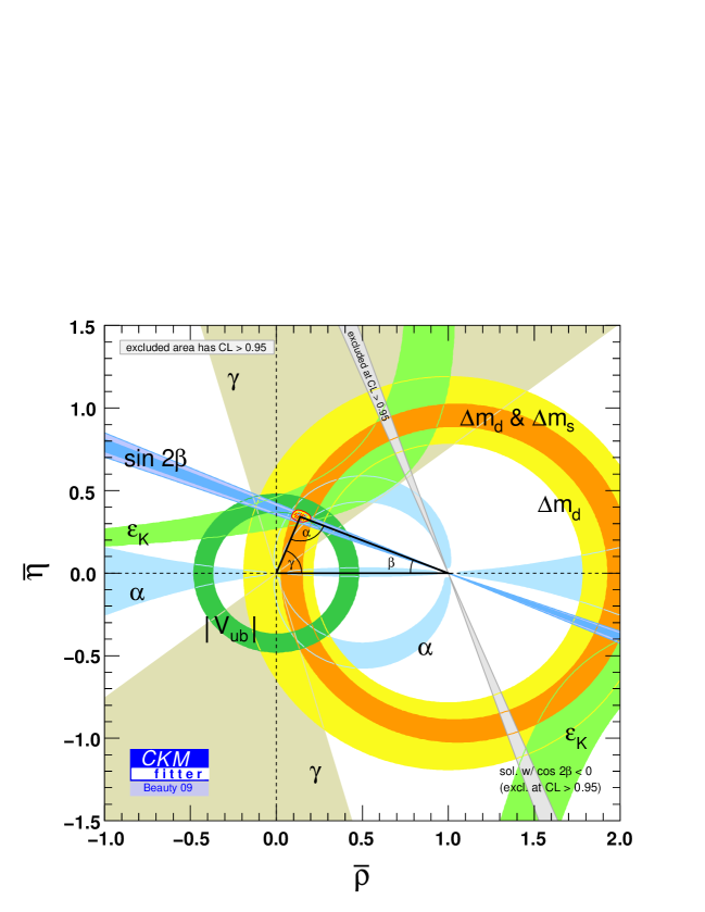
Figure 5: Global fit to the unitarity triangle based on all available data. (Taking from the CKMfitter group website, ckmfitter.in2p3.fr.)

The most important implication of this triumph of theoretical and experimental physics is the following statement: The Cabibbo-Kobayashi-Maskawa mechanism is the dominant source of flavor and CP violation in low-energy flavor-changing processes. This is a very important statement. Indeed the Nobel prize was awarded to Kobayashi and Maskawa in 2008 because it is now experimentally proven that the KM phase is the one which explains the observed CP violation in Nature.

VI.2 Instead of a summary: The NP flavor problem

The success of the SM can be seen as a proof that it is an effective low energy description of Nature. There are, however, many reasons to suspect that the SM has to be extended. A partial list includes the hierarchy problem, the strong CP problem, baryogenesis, gauge coupling unification, the flavor puzzle, neutrino masses, and gravity. We are therefore interested in probing the more fundamental theory. One way to go is to search for new particles that can be produced at yet unreached energies. Another way to look for new physics is to search for indirect effects of heavy unknown particles. Flavor physics is used to probe such indirect signals of physics beyond the SM.

In general, flavor bounds provide strong constraints on new physics models. This fact is called “the new physics flavor problem”. The problem is actually the mismatch between the new physics scale that is required in order to solve the hierarchy problem and the one that is needed in order to satisfy the experimental bounds from flavor physics.

In order to understand what the new physics flavor problem is, let us first recall the hierarchy problem. In order to prevent the Higgs mass from getting a large radiative correction, new physics must appear at a scale that is a loop factor above the weak scale

$$\Lambda\lesssim 4\pi m_{W}\sim 1\;{\rm TeV}.$$ (108)

Here, and in what follows, $\Lambda$ represents the new physics scale. Note that such TeV new physics can be directly probed in collider searches.

While the SM scalar sector is unnatural, its flavor sector is impressively successful. This success is linked to the fact that the SM flavor structure is special. As we already mentioned, the charged current interactions are universal (in the mass basis, this is manifest through the unitarity of the CKM matrix) and FCNCs are highly suppressed: they are absent at the tree level and at the one loop level they are further suppressed by the GIM mechanism. These special features are important in order to explain the observed pattern of weak decays. Thus, any extension of the SM must conserve these successful features.

Consider a generic new physics model, where the only suppression of FCNCs processes is due to the large masses of the particles that mediate them. Naturally, these masses are of the order of the new physics scale, $\Lambda$. Flavor physics, in particular measurements of meson mixing and CP violation, puts severe constraints on $\Lambda$. In order to find these bounds we take an effective field theory approach. At the weak scale we write all the non-renormalizable operators that are consistent with the gauge symmetry of the SM. In particular, flavor-changing four Fermi operators of the form (the Dirac structure is suppressed)

$${q_{1}\bar{q}_{2}q_{3}\bar{q}_{4}\over\Lambda^{2}},$$ (109)

are allowed. Here $q_{i}$ can be any quark as long as the electric charges of the four fields in Eq. (109) sum up to zero. We emphasize that there is no exact symmetry that can forbid such operators. This is in contrast to operators that violate baryon or lepton number that can be eliminated by imposing symmetries like $U(1)_{B-L}$ or R-parity. The strongest bounds are obtained from meson mixing and CP-violation measurements. Depending on the mode we find bounds of the order

$$\Lambda\gtrsim\mbox{few}\;\times 10^{4}{\mbox{~{}TeV}}.$$ (110)

There is tension between the new physics scale that is required in order to solve the hierarchy problem, Eq. (108), and the one that is needed in order not to contradict the flavor bounds, Eq. (110). The hierarchy problem can be solved with new physics at a scale $\Lambda\sim 1$ TeV. Flavor bounds, on the other hand, require $\Lambda\gtrsim 10^{4}$ TeV. This tension implies that any TeV scale new physics cannot have a generic flavor structure. This is the new physics flavor problem.

Flavor physics has been mainly an input to model building, not an output. The flavor predictions of any new physics model are not a consequence of its generic structure but rather of the special structure that is imposed to satisfy the severe existing flavor bounds. It is clearly a very interesting open question to determine the NP model and how it deals with flavor.

VI.3 Concluding remarks

This is a good time to finish the lectures. I hope that you gained some understanding of flavor physics, how it was used to shape the SM as we know it, and why it is so important in our quest to find the theory that extends the SM. In the near future we expect more data in the energy frontier, as well as more flavor data. It can be really fun to see how the two can work together to show us what Nature is at really short distances, that is, to help us in getting a better answer to the fundamental question of physics

$${\cal L}=?$$ (111)

References

- (1) O. Gedalia and G. Perez, “TASI 2009 Lectures - Flavor Physics,” arXiv:1005.3106 [hep-ph].
- (2) G. Isidori, “B physics in the LHC era,” arXiv:1001.3431 [hep-ph].
- (3) A. J. Buras, “Flavour Theory: 2009,” arXiv:0910.1032 [hep-ph].
- (4) U. Nierste, “Three Lectures on Meson Mixing and CKM phenomenology,” arXiv:0904.1869 [hep-ph].
- (5) M. Artuso, E. Barberio and S. Stone, “ Meson Decays,” PMC Phys. A 3, 3 (2009) [arXiv:0902.3743 [hep-ph]].
- (6) Y. Nir, “Probing new physics with flavor physics (and probing flavor physics with new physics),” arXiv:0708.1872 [hep-ph].
- (7) A. Hocker and Z. Ligeti, “CP violation and the CKM matrix,” Ann. Rev. Nucl. Part. Sci. 56, 501 (2006) [arXiv:hep-ph/0605217].
- (8) M. Neubert, “Effective field theory and heavy quark physics,” arXiv:hep-ph/0512222.
- (9) Y. Nir, “CP violation in meson decays,” arXiv:hep-ph/0510413.
- (10) A. J. Buras, “Flavour physics and CP violation,” arXiv:hep-ph/0505175.
- (11) Z. Ligeti, “Introduction to heavy meson decays and CP asymmetries,” In the Proceedings of 30th SLAC Summer Institute on Particle Physics: Secrets of the B Meson (SSI 2002), SLAC, Menlo Park, California, 5-16 Aug 2002, pp L02 [arXiv:hep-ph/0302031].
- (12) I. I. Y. Bigi and A. I. Sanda, “CP violation,” Camb. Monogr. Part. Phys. Nucl. Phys. Cosmol. 9, 1 (2000).
- (13) G. C. Branco, L. Lavoura and J. P. Silva, “CP violation,” Int. Ser. Monogr. Phys. 103, 1 (1999).
- (14) The Review of Particle Physics C. Amsler et al. (Particle Data Group), Physics Letters B667, 1 (2008). Recent updates can be found online at pdg.lbl.gov.