Method to circumvent the neutron gas problem
in the BCS treatment for nuclei far from stability

Abstract

Extending the Kruppa’s prescription for the continuum level density, we have recently improved the BCS method with seniority-type pairing force in such a way that the effects of discretized unbound states are properly taken into account for finite depth single-particle potentials. In this paper, it is further shown, by employing the Woods-Saxon potential, that the calculation of spatial observables like nuclear radius converges as increasing the basis size in the harmonic oscillator expansion. Namely the disastrous problem of a “particle gas” surrounding nucleus in the BCS treatment can be circumvented. In spite of its simplicity, the new treatment gives similar results to those by more elaborate Hartree-Fock-Bogoliubov calculations; e.g., it even mimics the pairing anti-halo effect. The obtained results as well as the reason of convergence in the new method are investigated by a variant of the Thomas-Fermi approximation within the limited phase space which corresponds to the harmonic oscillator basis truncation.

I Introduction

The advent of new radioactive beam facilities makes it increasingly interesting to study unstable nuclei near the neutron or proton drip line. One of their specific features is weak binding of constituent nucleons, which leads to spatially extended nuclear profiles and a striking phenomenon of the neutron halo Tani96 . Among many issues expected in researches of nuclei far from the stability DobNaz98 ; Dob99 , the pairing correlation plays a special role because virtual scatterings into continuum states occur more easily. The basic quantity concerning the spatial distribution of nucleons is the nuclear radius, which is also a prerequisite for the analysis of reaction cross sections Tani96 . However, its theoretical evaluation in the presence of pairing correlation is not straightforward due to the fact that the continuum states, into which weakly bound nucleons virtually scatter, occupy infinite volume. In fact, the calculated radius is unreasonably large or divergent because of finite occupation probabilities of unbound states in the simple-minded BCS treatment; the so-called “neutron gas” problem, the solution of which requires the more sophisticated Hartree-Fock-Bogoliubov (HFB) theory DFT84 ; DNW96 ; DNW96a .

A similar problem exists for the Strutinsky shell correction calculation with finite depth potential BFN72 , where the smoothed part of binding energy does not converge when increasing the size of the single-particle basis: The finite occupation probabilities of continuum states are required for extracting the smooth part, but the level density of unbound states is infinite, which leads to divergence of the Strutinsky smoothed energy. An efficient method to avoid this problem was introduced by Kruppa Kru98 , and was used in the shell correction method VKN00 . The idea of the method is to calculate the so-called continuum level density as a difference between the level densities obtained by diagonalizing the full Hamiltonian including a finite depth potential and the free Hamiltonian. By employing the harmonic oscillator expansion, it was shown for the Woods-Saxon potential that the smoothed energy calculated by the Kruppa method well converges as increasing the size of basis VKN00 .

Recently, three of the authors of this paper have proposed a new method of BCS calculation TST10 , which is free from the divergence as increasing the model space, by utilizing the similar idea to Kruppa’s. In Ref. TST10 not only the treatment of pairing correlation but all the other procedures in the microscopic-macroscopic method for the calculation of nuclear binding energy are reexamined and improved. In this paper, we further show that the new method is capable of calculating the spatial observables like the nuclear radius without the problem of particle gas surrounding nucleus.

II Kruppa prescription for expectation values of one-body operators

II.1 Basic idea

In the Kruppa’s prescription Kru98 , the level density is replaced as

$$g(\epsilon)\quad\Rightarrow\quad g^{\rm K}(\epsilon)=g(\epsilon)-g_{0}(\epsilon)\equiv\sum_{i=1}^{M}\delta\left(\epsilon-\epsilon_{i}\right)-\sum_{j=1}^{M}\delta(\epsilon-\epsilon^{0}_{j}),$$ (1)

where $\epsilon_{i}$ and $\epsilon^{0}_{j}$ are the eigenvalues of the full and the free Hamiltonians, respectively. In the following, we are mainly concerned with neutrons, but it should be reminded for protons that the Coulomb potential is included in the free Hamiltonian, i.e., “free” here means that the nuclear potential is left out. The eigenvalues in Eq. (1) are calculated by diagonalizations with the harmonic oscillator basis, and $M$ is the total number of the basis states commonly used in the two diagonalizations. Both the full and free level densities, $g(\epsilon)$ and $g_{0}(\epsilon)$, are divergent as increasing the basis size ($M\rightarrow\infty$) for the positive single-particle energy, $\epsilon>0$. It is shown for the Woods-Saxon potential Kru98 that their difference $g^{\rm K}(\epsilon)$ remains finite, and converges, in the spherical case, to the well-known expression in terms of the scattering phase shift $\delta_{lj}(\epsilon)$,

$$\frac{1}{\pi}\sum_{lj}(2j+1)\frac{d\delta_{lj}(\epsilon)}{d\epsilon}.$$ (2)

The great merit of Eq. (1) is that it can be easily applied to the deformed cases (see Ref. Kru98 for the corresponding expression to Eq. (2) in terms of the scattering S-matrix in such general cases).

Extending the idea of subtracting the free contribution in Eq. (1), we propose to calculate the expectation value of an arbitrary one-body observable $O$ by a similar replacement as

$$\langle O\rangle\quad\Rightarrow\quad\langle O\rangle^{\rm K}=\langle O\rangle-\langle O\rangle_{0},$$ (3)

where the first (second) term is a summation of the expectation values with respect to the wave functions calculated by diagonalizing the full (free) Hamiltonian multiplied with the occupation numbers. Note that, in the independent particle approximation, e.g., the Hartree-Fock (HF) theory, the second term does not contribute for bound systems, i.e., if the Fermi energy is below the particle threshold. The free contribution manifests itself when the occupation probabilities of continuum states are non-zero due to the residual interactions, e.g., in the case of BCS treatment for pairing correlations.

Although generalizations are possible, we consider in this work the following seniority-type separable pairing interaction,

$$V_{\rm pair}=-G\,\hat{P}^{\dagger}\hat{P},\qquad\hat{P}^{\dagger}=\sum_{i>0}f_{\rm c}(\epsilon_{i})\,c^{\dagger}_{i}c^{\dagger}_{\bar{i}},$$ (4)

where $\bar{i}$ represents the time-reversed state of $i$, forming a time reversal pair $(i\bar{i})$ (they are degenerate in energy, $\epsilon_{i}=\epsilon_{\bar{i}}$), and $\sum_{i>0}$ means the sum is taken over all the pairs. A cutoff of the model space is necessary for such a pairing interaction, and it is realized by introducing a smooth cutoff function BFH85 , $f_{\rm c}(\epsilon)$ (we use a different form from that of Ref. BFH85 ), defined by

$$f_{\rm c}(\epsilon)=\frac{1}{2}\left[1+{\rm erf}\left(\frac{\epsilon-\tilde{\lambda}+\Lambda_{\rm l}}{d_{\rm cut}}\right)\right]^{1/2}\left[1+{\rm erf}\left(\frac{-\epsilon+\tilde{\lambda}+\Lambda_{\rm u}}{d_{\rm cut}}\right)\right]^{1/2},$$ (5)

where ${\displaystyle{\rm erf}(x)\equiv\frac{2}{\sqrt{\pi}}\int_{0}^{x}e^{-t^{2}}dt}$ is the error function. We use the cutoff parameters of the pairing model space, $\Lambda_{\rm u}=\Lambda_{\rm l}=1.2\,\hbar\omega$ and $d_{\rm cut}=0.2\,\hbar\omega$, with $\hbar\omega=41/A^{1/3}$ MeV. The predefined parameter $\tilde{\lambda}$ in the cutoff function (5) is chosen to be the smoothed Fermi energy obtained by the Strutinsky smoothing procedure, see Ref. TST10 for details.

The gap equation can be derived from the variational principle with the number constraint,

$$\Delta=G\langle\hat{P}^{\dagger}\rangle,\qquad\mbox{and}\qquad N=\langle\hat{N}\rangle,$$ (6)

where $N$ is the neutron or proton number to be fixed. Applying the prescription (3), the modified gap and number constraint equations are obtained:

$$\frac{2}{G} = \sum_{i>0}\left[\frac{f_{\rm c}(\epsilon_{i})^{2}}{E(\epsilon_{i})}-\frac{f_{\rm c}(\epsilon^{0}_{i})^{2}}{E(\epsilon^{0}_{i})}\right],$$ (7)

$$N = \sum_{i>0}\left[2v^{2}(\epsilon_{i})-2v^{2}(\epsilon^{0}_{i})\right].$$ (8)

Here the BCS quasiparticle energy and occupation probability are given, as usual, by

$$E(\epsilon)={\sqrt{(\epsilon-\lambda)^{2}+f_{\rm c}(\epsilon)^{2}\Delta^{2}}},\qquad v^{2}(\epsilon)=\frac{1}{2}\left(1-\frac{\epsilon-\lambda}{E(\epsilon)}\right).$$ (9)

From these equations, the pairing gap and the chemical potential, ($\Delta,\lambda$), are determined for a given pairing strength $G$. The second terms in the square brackets in Eqs. (7) and (8) are the extra (negative) contributions form the free spectra. We call this new way of the BCS treatment Kruppa-BCS method, and the resultant equation Kruppa-BCS equation. The consequences of this Kruppa-BCS equation have been investigated in detail in Ref. TST10 . As long as the chemical potential is well below the free particle threshold (minimum of $\{\epsilon^{0}_{i},i=1,2,...\}$), the Kruppa-BCS equation has a unique solution and can be solved in the same way as the ordinary BCS equation. It is shown that the calculated pairing gaps with this new method converge to reasonable values for large basis size in contrast to those with the ordinary BCS equation, which strongly depend on the size of basis and hardly applicable to the calculations with large basis size NWD94 . See Ref. TST10 for a comprehensive discussion.

II.2 Root mean square radii and deformation parameters

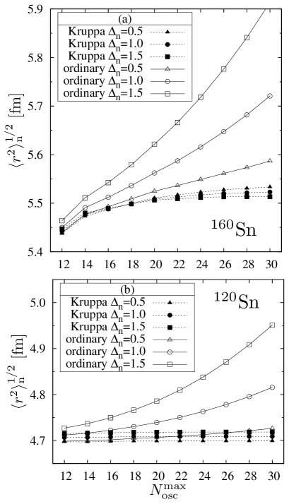
Figure 1: Neutron’s rms radii as functions of the maximum harmonic oscillator quantum number $N_{\rm osc}^{\rm max}$, which specifies the size of basis. Those calculated by the ordinary prescription, $\langle r^{2}\rangle_{\rm n}$, and the Kruppa prescription, $\langle r^{2}\rangle^{\rm K}_{\rm n}$ in Eq. (10), are included for a near drip-line nucleus ¹⁶⁰Sn, the panel (a), and for a $\beta$-stable nucleus ¹²⁰Sn, (b). Both nuclei are spherical. The neutron pairing gap is fixed to be either $\Delta_{\rm n}=0.5$, 1.0, or 1.5 MeV.

Once the pairing gap and the chemical potential, $(\Delta,\lambda)$, are obtained by the Kruppa-BCS equation (7) and (8), the expectation value of one-body observables can be calculated within the BCS treatment; for example, the root mean square (rms) radius by

$$\langle r^{2}\rangle^{\rm K}=\langle r^{2}\rangle-\langle r^{2}\rangle_{0}=\frac{1}{N}\sum_{i>0}\left[\langle i|r^{2}|i\rangle\,2v^{2}(\epsilon_{i})-\langle i|r^{2}|i\rangle_{0}\,2v^{2}(\epsilon^{0}_{i})\right],$$ (10)

where the diagonal matrix elements $\langle i|r^{2}|i\rangle$ and $\langle i|r^{2}|i\rangle_{0}$ are with respect to the Woods-Saxon and free spectra, respectively. Figure 1 shows the calculated neutron radii for a stable nucleus ¹²⁰Sn and an unstable nucleus ¹⁶⁰Sn in the lower and upper panels, respectively. They are depicted as functions of the maximum value of the harmonic oscillator quantum number, $N_{\rm osc}^{\rm max}$, specifying the model space. As for the Woods-Saxon potential, we use the parameter set recently developed by Ramon Wyss RWyss , which gives similar density distributions, both for neutrons and protons, to those obtained by Skyrme and Gogny HF calculations. In order to see the impact of the pairing correlation on the radius, the pairing gap in this calculation is kept constant to the values $\Delta_{\rm n}=0.5$, 1.0, and 1.5 MeV, and only the number constraint equation (8) is solved for determining the chemical potential $\lambda_{\rm n}$. The Kruppa mean value $\langle r^{2}\rangle^{\rm K}_{\rm n}$ in Eq. (10) and the ordinary mean value $\langle r^{2}\rangle_{\rm n}$ are compared. Note that for the calculation of the latter, the ordinary number equation is solved so that the chemical potentials in the calculations of two radii, $\langle r^{2}\rangle^{\rm K}_{\rm n}$ and $\langle r^{2}\rangle_{\rm n}$, are generally different. As is quite evident from Fig. 1, the calculated radii by the ordinary method diverge as increasing the basis size $N_{\rm osc}^{\rm max}$. The divergence is more rapid for larger pairing gaps. There is no way to obtain meaningful results even for the stable nucleus ¹²⁰Sn. This is nothing but the problem of the ”neutron gas” surrounding the nucleus DFT84 ; DNW96 ; DNW96a . In contrast, the radii calculated by the Kruppa method converge to definite values. Comparing with Fig. 15 in Ref. DFT84 , our Kruppa results nicely corresponds to those of the HFB calculation, although the coordinate space is utilized in Ref. DFT84 and the box size instead of $N_{\rm osc}^{\rm max}$ is changed to demonstrate the convergence.

It is sometimes recommended to be content with a small model space BFN72 ; MNM95 , like $N_{\rm osc}^{\rm max}\approx 12$, for finite depth potentials, because the plateau condition for the shell correction energy is not met with larger model spaces. Such a backward idea may work for stable nuclei, but it is clear from Fig. 1 (a) that the space $N_{\rm osc}^{\rm max}\approx 12$ is not enough to calculate accurately the rms radius of ¹⁶⁰Sn, and using a larger model space requires inevitably the Kruppa method.

Another interesting feature of the Kruppa calculations seen in Fig. 1 is that the radius of stable nucleus stretches for larger pairing gaps while that of the nucleus near drip-line shrinks, although the absolute amount of changes is very small. The stretching of the radius due to the pairing correlation is well-known: The pairing induces the couplings to particle states above the Fermi surface, whose rms radii are larger in average than those of hole states, and increased occupation probabilities of particles and decreased occupation probabilities of holes make the expectation value of radius larger (see Fig. 4 (c) and discussions in Sec.II.4). In spite of this effect, the radius of near drip-line nucleus ¹⁶⁰Sn shrinks. We believe that this is related to the interesting “pairing anti-halo” effect BDP00 in the HFB theory, and will come back to this point later in Sec. II.5.

Figure 2: Neutron’s deformation parameter (11) as functions of the maximum harmonic oscillator quantum number $N_{\rm osc}^{\rm max}$. Those calculated by the ordinary and the Kruppa prescriptions are included for a near drip-line nucleus ²⁰⁸Dy, the panel (a), and a $\beta$-stable nucleus ¹⁶⁰Dy, (b). Both nuclei are axially deformed. The pairing gap, $\Delta_{\rm n}=0.5$, 1.0, and 1.5 MeV, are employed.

In order to further illustrate the importance of the Kruppa prescription of Eq. (3), presented in Fig. 2 are examples of calculation for the quadrupole deformation parameter defined as a ratio of the quadrupole moment to the mean square radius,

$$\beta=\frac{4\pi}{5}\,\frac{\langle r^{2}Y_{20}\rangle}{\langle r^{2}\rangle},\qquad\beta^{\rm K}=\frac{4\pi}{5}\,\frac{\langle r^{2}Y_{20}\rangle^{\rm K}}{\langle r^{2}\rangle^{\rm K}}\equiv\frac{4\pi}{5}\,\frac{\langle r^{2}Y_{20}\rangle-\langle r^{2}Y_{20}\rangle_{0}}{\langle r^{2}\rangle-\langle r^{2}\rangle_{0}}.$$ (11)

In the upper and lower panels ((a) and (b)) the results for ²⁰⁸Dy and ¹⁶⁰Dy are depicted, respectively, as functions of the basis size. Both nuclei are axially deformed, and the deformation parameters used in the Woods-Saxon potential are $(\beta_{2},\beta_{4})=(0.244,0.053)$ and $(0.269,0.035)$, respectively, which are obtained by the improved microscopic-macroscopic method of Ref. TST10 . As in Fig. 1, the fixed pairing gaps of $\Delta_{\rm n}=0.5$, 1.0, and 1.5 MeV are used. Apparently, the quadrupole moment as well as the radius diverges as increasing the basis size due to the neutron gas surrounding the nucleus, if being calculated by the ordinary BCS treatment. One might expect that their ratio would converge to the correct value. It is not the case, however, even in stable nuclei, and the error is larger in neutron rich nuclei, amounting to about 10% for $\Delta_{\rm n}=1.5$ MeV and $N_{\rm osc}^{\rm max}=30$ in ²⁰⁸Dy. If the Kruppa prescription is used, the results with $N_{\rm osc}^{\rm max}\approx 12$ are already sufficiently accurate. Namely, compared with the radius or the quadrupole moment itself, the convergence of the deformation parameter as their ratio against the increase of the model space is much faster. Therefore it is better to use the Kruppa method even for calculations with $N_{\rm osc}^{\rm max}\approx 12$.

II.3 Semiclassical consideration

In the case of the single-particle level density, the convergence of the Kruppa density (1) to the exact density (2) in the limit of infinite model space, $M\rightarrow\infty$ (continuum limit), can be proved rigorously Kru98 ; Shl92 ; TO75 . Recently, we have shown the convergence more pictorially by employing a variant of the semiclassical (Thomas-Fermi) approximation. We call it the oscillator-basis Thomas-Fermi (OBTF) approximation TST10 , which is suitable to treat the problem with the truncation in terms of the harmonic oscillator basis. In the following, we briefly sketch this OBTF approximation, and show that the Kruppa prescription (3) for the expectation value of any spatial observables like the radius is convergent as increasing the basis size, $N_{\rm osc}^{\rm max}\rightarrow\infty$.

The basic quantity in the Thomas-Fermi approximation is the phase space distribution function RS80 . Because the momentum distribution is isotropic in the nuclear ground state RS80 , the distribution function depends only on the magnitude of the momentum variable, which one can transform to the energy $\epsilon$. Thus the distribution function for the single-particle Hamiltonian, ${\displaystyle H=\frac{\bm{p}^{2}}{2m}+V(\bm{r})}$, is written, using the Heaviside step function $\theta(x)$, as

$$f_{\!\!\phantom{.}{}_{\mbox{\tiny TF}}}(\bm{r},\epsilon)=\frac{(2m)^{3/2}}{2\pi^{2}\hbar^{3}}\left|\epsilon-V(\bm{r})\right|^{1/2}\theta\left(\epsilon-V(\bm{r})\right),$$ (12)

with which the Thomas-Fermi level density can be obtained as ${\displaystyle g_{\!\!\phantom{.}{}_{\mbox{\tiny TF}}}(\epsilon)=\int f_{\!\!\phantom{.}{}_{\mbox{\tiny TF}}}(\bm{r},\epsilon)d^{3}r}$. In the OBTF approximation, the distribution function is modified to incorporate the effect of the limited phase space corresponding to the truncated harmonic oscillator (HO), i.e.,

$$f_{\!\!\phantom{.}{}_{\mbox{\tiny OB}}}(\bm{r},\epsilon)=f_{\!\!\phantom{.}{}_{\mbox{\tiny TF}}}(\bm{r},\epsilon)\,\theta\left(\epsilon_{\rm kin}^{\rm max}(r)+V(\bm{r})-\epsilon\right).$$ (13)

Here the quantity $\epsilon_{\rm kin}^{\rm max}(r)$ is the local maximum kinetic energy of the isotropic HO potential, ${\displaystyle V_{\rm HO}(\bm{r})=\frac{1}{2}m\omega^{2}r^{2}}$,

$$\epsilon_{\rm kin}^{\rm max}(r)=\frac{1}{2}m\omega^{2}\left(R_{\rm max}^{2}-r^{2}\right)\theta\left(R_{\rm max}-r\right),$$ (14)

where the maximum radius $R_{\rm max}$ allowed in the HO potential is specified by the cutoff energy $\epsilon_{\rm cut}$, related to the maximum HO quantum number $N_{\rm osc}^{\rm max}$ of the basis truncation;

$$R_{\rm max}=\sqrt{\frac{2\epsilon_{\rm cut}}{m\omega^{2}}},\qquad\epsilon_{\rm cut}=\hbar\omega\left[(N_{\rm osc}^{\rm max}+1)(N_{\rm osc}^{\rm max}+2)(N_{\rm osc}^{\rm max}+3)\right]^{1/3}.$$ (15)

(Although the anisotropic HO basis is utilized in the actual calculation, it is enough to consider the isotropic HO potential for proving the convergence.) Thus, the infinite model space limit $N_{\rm osc}^{\rm max}\rightarrow\infty$ is realized by $R_{\rm max}\rightarrow\infty$ in $f_{\mbox{\tiny OB}}(\bm{r},\epsilon)$, and the OBTF level density ${\displaystyle g_{\!\!\phantom{.}{}_{\mbox{\tiny OB}}}(\epsilon)=\int f_{\!\!\phantom{.}{}_{\mbox{\tiny OB}}}(\bm{r},\epsilon)d^{3}r}$ is finite and calculable as long as $R_{\rm max}$ (or $N_{\rm osc}^{\rm max}$) is kept finite. Note that this is not the case for the usual Thomas-Fermi quantities; $g_{\!\!\phantom{.}{}_{\mbox{\tiny TF}}}(\epsilon)$ and $f_{\!\!\phantom{.}{}_{\mbox{\tiny TF}}}(\bm{r},\epsilon)$ are both infinite for the energy $\epsilon$ above the particle threshold due to the infinite spatial volume of the phase space. In the same way, the OBTF distribution function for the free Hamiltonian, $f^{0}_{\mbox{\tiny OB}}(\bm{r},\epsilon)$, is defined by dropping the potential $V(\bm{r})$ (or replacing it with the Coulomb potential for protons). The Kruppa level density in the OBTF approximation, $g^{\rm K}_{\mbox{\tiny OB}}(\epsilon)=g_{\mbox{\tiny OB}}(\epsilon)-g^{0}_{\mbox{\tiny OB}}(\epsilon)$, is obtained by the spatial integral of $f^{\rm K}_{\mbox{\tiny OB}}(\bm{r},\epsilon)=f_{\mbox{\tiny OB}}(\bm{r},\epsilon)-f^{0}_{\mbox{\tiny OB}}(\bm{r},\epsilon)$. Both level densities, $g_{\!\!\phantom{.}{}_{\mbox{\tiny OB}}}(\epsilon)$ and $g_{\!\!\phantom{.}{}_{\mbox{\tiny OB}}}^{0}(\epsilon)$, diverges as $R_{\rm max}\rightarrow\infty$, but the Kruppa density $g_{\!\!\phantom{.}{}_{\mbox{\tiny OB}}}^{\rm K}(\epsilon)$ remains finite for the potential $V(\bm{r})$ that vanishes rapidly enough as $|\bm{r}|\rightarrow\infty$ like the Woods-Saxon potential. It has been shown TST10 that, for single-particle energies satisfying $0<\epsilon<\epsilon_{\rm kin}^{\rm max}(\bm{r})+V(\bm{r})$ (assuming $V(\bm{r})\leq 0$) everywhere,

$$g_{\!\!\phantom{.}{}_{\mbox{\tiny OB}}}^{\rm K}(\epsilon)\approx\frac{(2m)^{3/2}}{2\pi^{2}\hbar^{3}}\int\left[\left(\epsilon-V(\bm{r})\right)^{1/2}-\epsilon^{1/2}\right]\,d^{3}r,$$ (16)

asymptotically in the limit of $R_{\rm max}\rightarrow\infty$.

It is straightforward to apply the OBTF approximation to the calculation of physical observables with pairing correlation (see, e.g., Ref. RS80 for the semiclassical treatment of the BCS theory). For a spatial one-body observable, $O(\bm{r})$, its Kruppa OBTF expectation value can be expressed as

$$\langle O\rangle^{\rm K}_{\mbox{\tiny OB}}=\int_{-\infty}^{\infty}g_{\!\!\phantom{.}{}_{\mbox{\tiny OB}}}^{\rm K}(\langle O\rangle;\epsilon)\,2v^{2}(\epsilon)\,d\epsilon,$$ (17)

where the BCS occupation probability $v^{2}(\epsilon)$ is given in Eq. (9), and the distribution of $\langle O\rangle$ with respect to the energy is defined by

$$g_{\!\!\phantom{.}{}_{\mbox{\tiny OB}}}^{\rm K}(\langle O\rangle;\epsilon)\equiv\int O(\bm{r})f_{\!\!\phantom{.}{}_{\mbox{\tiny OB}}}^{\rm K}(\bm{r},\epsilon)\,d^{3}r,$$ (18)

which reduces to the level density $g_{\!\!\phantom{.}{}_{\mbox{\tiny OB}}}^{\rm K}(\epsilon)$ for the case $O=1$. The problem of “particle gas” occurs at energies above the particle threshold, $\epsilon>0$, as in the same way as the level density. Then, similarly to Eq. (16), the quantity (18) converges asymptotically as $R_{\rm max}\rightarrow\infty$ to

$$g_{\!\!\phantom{.}{}_{\mbox{\tiny OB}}}^{\rm K}(\langle O\rangle;\epsilon)\approx\frac{(2m)^{3/2}}{2\pi^{2}\hbar^{3}}\int\left[\left(\epsilon-V(\bm{r})\right)^{1/2}-\epsilon^{1/2}\right]O(\bm{r})\,d^{3}r,$$ (19)

for the spatial observable $O(\bm{r})$ like the radius or the quadrupole moment (assuming the upper cutoff energy of the pairing model space by the function (5), $\approx\tilde{\lambda}+\Lambda_{u}$, is smaller than $\epsilon_{\rm kin}^{\rm max}(\bm{r})+V(\bm{r})$ everywhere). This guarantees the convergence of the Kruppa expectation value $\langle O\rangle^{\rm K}_{\mbox{\tiny OB}}$ in the BCS treatment.

II.4 Convergence in the Kruppa prescription

In order to see how the calculated rms radii converge as functions of $N_{\rm osc}^{\rm max}$, we have done many test calculations Ono10 . Generally, the rate of convergence is fast for stable nuclei as is already shown in Fig. 1 (b), while it is slow for neutron rich nuclei depending on what kind of orbits exist near the Fermi surface. Figure 3 includes four selected examples of nuclei near the neutron drip-line (note the extension of the abscissa to $N_{\rm osc}^{\rm max}=40$ and the enlarged scale of ordinate compared with Fig. 1). All nuclei except ²⁰⁸Dy are spherical. The radius has converged within accuracy of about 0.5% already at $N_{\rm osc}^{\rm max}\approx 20$ in most cases where the pairing correlation is effective ($\Delta\geq 1$ MeV). The very slow convergence in the weak pairing correlations, e.g., the case of $\Delta_{\rm n}=0.5$ MeV in ⁸⁸Ni (panel (a)) is due to the filling of the “halo” orbit near the Fermi surface, e.g., $\nu 3s_{1/2}$ (and $\nu 2d_{3/2}$) in ⁸⁸Ni. The description of such spatially extended wave functions requires many oscillator basis states. Another striking feature shown in Fig. 3 is that the calculated radii with the largest basis size ($N_{\rm osc}^{\rm max}=40$) are always smaller for larger pairing gaps: It is found that this calculated feature is rather general for nuclei near the drip-line, and mimics the pairing anti-halo effect in the HFB theory. We discuss this point in more detail in Sec. II.5.

Figure 3: Convergence of neutron’s rms radii calculated by the Kruppa method as functions of $N_{\rm osc}^{\rm max}$ for various nuclei near the drip-line, ⁸⁸Ni (a), ¹²⁶Zr (b), ${208}$Dy (c), and ²⁵⁶Hg (d). Only ²⁰⁸Dy is axially deformed. The values of neutron pairing gap used are $\Delta_{\rm n}=0.5$, 1.0, 1.5, and 2.0 MeV.

Figure 4: The distribution of $\langle r^{2}\rangle$ with respect to the single-particle energy $\epsilon$ (c.f. Eqs. (18), (20)), panel (a), the level density, panel (b), and the rms radius of orbits at $\epsilon$ defined in Eq. (22), panel (c), as functions of $\epsilon$ for the spherical drip-line nucleus ¹²⁶Zr. The OBTF and Strutinsky smoothed ones with the smoothing parameter $\gamma=0.8\,\hbar\omega$ and $1.8\,\hbar\omega$ and with the six order of the curvature correction polynomial ($p=3$ in Ref. TST10 ) are included. $N_{\rm osc}^{\rm max}=40$ is used for the basis size.

In Ref. TST10 the OBTF level density is compared with the Strutinsky smoothed level density to clarify the convergence mechanism by the Kruppa prescription, i.e., by subtracting the contributions of free spectra. It is instructive to perform a similar analysis for the mean square radius. The microscopic quantity corresponding to the distribution of $\langle O\rangle=\langle r^{2}\rangle$ in Eq. (18) is

$$g^{\rm K}(\langle r^{2}\rangle;\epsilon)=\sum_{i>0}\left[\langle i|r^{2}|i\rangle\,\delta(\epsilon-\epsilon_{i})-\langle i|r^{2}|i\rangle_{0}\,\delta(\epsilon-\epsilon^{0}_{i})\right],$$ (20)

with which the mean square radius in Eq. (10) is calculated by integral

$$\langle r^{2}\rangle^{\rm K}=\frac{1}{N}\int_{-\infty}^{\infty}g^{\rm K}(\langle r^{2}\rangle;\epsilon)\,2v^{2}(\epsilon)\,d\epsilon.$$ (21)

In Fig. 4, we depict the Strutinsky smoothed quantity of Eq. (20) and its OBTF approximation (panel (a)), as well as the corresponding level densities (panel (b)). The large model space with $N_{\rm osc}^{\rm max}=40$ is used. As for the OBTF approximation, we use Eq. (19) with $O=r^{2}$ for $\epsilon>0$ and the conventional Thomas-Fermi expression, i.e., $\left(\epsilon-V(r)\right)^{1/2}-\epsilon^{1/2}$ in the square brackets in Eq. (19) being replaced with $\left|\epsilon-V(r)\right|^{1/2}\theta(\epsilon-V(r))$, for $\epsilon<0$, considering only the central part of the Woods-Saxon potential with spherical symmetry for $V(r)$ TST10 . The sharp cusp behaviors at $\epsilon=0$ seen in all panels of Fig. 4 are due to the threshold effect characteristic in the OBTF approximation TST10 .

As it was already discussed in detail in Ref. TST10 , apart from the oscillation and the cusp at $\epsilon=0$, the OBTF approximation reproduces nicely the microscopic level density smoothed with $\gamma=1.8\,\hbar\omega$. It also reproduces, but less nicely, the quantity $g(\langle r^{2}\rangle;\epsilon)$. The result of the smoothing with $\gamma=1.8\,\hbar\omega$ is larger than the OBTF approximation in $-20$ MeV $\leq\epsilon\leq-2$ MeV (where the error becomes largest) and $\epsilon\geq 2$ MeV (from where there is little contribution because of the vanishing occupation probability $v^{2}(\epsilon)$). It is helpful to introduce a physically more meaningful quantity, “rms radius of orbits at the single-particle energy $\epsilon$”, defined by

$$\langle r^{2}\rangle^{1/2}(\epsilon)\equiv\sqrt{g^{\rm K}(\langle r^{2}\rangle;\epsilon)/g^{\rm K}(\epsilon)},$$ (22)

which is also depicted in Fig. 4 (c). The corresponding quantity in the HFB theory is the rms radius of the canonical basis states plotted versus the expectation value of the mean field Hamiltonian, whose gradually increasing tendency above the particle threshold is shown in Ref. Taj04 . From Eqs. (16) and (19) (and corresponding ones in the conventional Thomas-Fermi approximation for $\epsilon<0$), the Kruppa OBTF radius $\langle r^{2}\rangle^{1/2}(\epsilon)$ in Eq. (22) monotonically increases in $\epsilon<0$, takes a maximum value $\langle r^{2}\rangle^{1/2}_{\sqrt{V}}$ at $\epsilon=0$ and goes to an asymptotic value $\langle r^{2}\rangle^{1/2}_{V}$ as $\epsilon\rightarrow\infty$, where (assuming the spherical symmetry)

$$\langle r^{2}\rangle_{\sqrt{V}} \equiv \int\sqrt{-V(r)}\,r^{4}dr/\int\sqrt{-V(r)}\,r^{2}dr,$$ (23)

$$\langle r^{2}\rangle_{V} \equiv \int(-V(r))\,r^{4}dr/\int(-V(r))\,r^{2}dr.$$ (24)

The microscopic Strutinsky smoothed radii in Fig. 4 (c) behave similarly to the OBTF expression except a complete smearing out of the cusp (with $\gamma=1.8\,\hbar\omega$) and an increasing overestimation at positive energies. The monotonically increasing trend of the quantity $\langle r^{2}\rangle^{1/2}(\epsilon)$ in $\epsilon<0$ (smoothing width $\gamma=0.8\,\hbar\omega$) clearly indicates that the orbit with larger energy has larger radius in average, which leads to the increase of the total nuclear radius for larger pairing gap.

The analyses in this subsection have shown how finite results for rms radii are obtained with the Kruppa prescription in the OBTF approximation and in which ways the quantum mechanical results deviate from the results of this approximation.

II.5 Pairing anti-halo like effect

It is well-known that the occupation of the weakly bound orbit with low orbital angular momentum, typically $s$-orbits, leads to the nuclear halo and many examples are experimentally observed in light nuclei Tani96 . However, it is speculated that the increased pairing correlation binds these halo orbits more tightly and prevents the appearance of halo phenomena in heavier nuclei BDP00 . To confirm this speculation is one of the most interesting subjects both theoretically and experimentally.

Figure 5: Neutron’s rms radii calculated by the Kruppa method with $N_{\rm osc}^{\rm max}=40$ for the Ni–isotopes near the drip-line. The Kruppa-BCS equation is solved to obtain the selfconsistent pairing gap, where the pairing force strength is determined by the improved average gap method of Ref. TST10 . The results without including the pairing correlation are also included.

In this respect, the Ni–isotopes are very interesting, whose drip-line may possibly be reached in near future. The coordinate-space HFB calculation in Ref. GSG01 , as an example, showed that indeed an abrupt increase of radii in the HF calculation is diminished by including the pairing correlation.

We have calculated the same quantity with the Kruppa method in the following way. The calculated neutron drip-line based on the original Woods-Saxon potential RWyss is slightly inside of the expected position. Therefore, the modification of its depth has been done according to a new systematic method developed in Ref. TST10 ; then the drip-line isotope is the $A=92$ nucleus (the $A=94$ nucleus is unbound), while it is the $A=90$ nucleus in the calculation of Ref. GSG01 . The Kruppa-BCS equation is solved for each nucleus, and the full microscopic-macroscopic (Strutinsky shell correction) method is applied with the results that all the isotopes are spherical. The average pairing gap method with $\Delta=13/\sqrt{A}$ MeV is used to fix the strength $G$, and the calculated pairing gaps are $\Delta_{\rm n}\approx$ 1.2 to 1.7 MeV, monotonically increasing from the $A=80$ to $A=92$ isotopes. We depict the result of our Kruppa calculations for radii of Ni–isotopes in Fig. 5. Although the absolute values of radii are slightly larger in our calculations, the behavior of how the radii increase is very similar to the calculation shown in Fig. 7 of Ref. GSG01 .

It may be worthwhile mentioning that a BCS treatment with including only the resonance orbits (the resonance-BCS) is tested in Ref. GSG01 : The calculated radii are not good approximation to those of HFB (no pairing anti-halo effect is reproduced), although the obtained binding energy is very good. This clearly indicates the subtlety of the neutron gas problem in the conventional BCS treatment, and we should be very careful to calculate such quantities for weakly bound systems DobNaz98 .

The pairing anti-halo effect in the HFB theory BDP00 is a result of real shrinkage of the hole component of the quasiparticle orbits due to the selfconsistent modification of the potentials. Apparently, such effect is absent in the Kruppa prescription because the BCS treatment of quasiparticle does not change the spatial distribution of each single-particle orbit. Then it is surprising that a similar shrinkage of the rms radius comes out from the Kruppa-BCS calculation. The key to understand the reason is the rms radius $\langle r^{2}\rangle^{1/2}(\epsilon)$ defined in Eq. (22) and depicted in Fig. 4 (c). Note that the total mean square radius is calculated as an integral (21) with the weight of the BCS occupation probability $v^{2}(\epsilon)$, which is a step function at $\epsilon=\lambda$ smeared with the pairing gap $\Delta$. Therefore, if the quantity $\langle r^{2}\rangle^{1/2}(\epsilon)$ is larger for $\epsilon<\lambda$ and smaller for $\epsilon>\lambda$, the increase of $\Delta$ leads to the effective shrinkage of the total mean square radius. In fact, this behavior, i.e., the local decrease near the particle threshold $\epsilon\approx 0$, is observed in the result of smaller smoothing width $\gamma=0.8\,\hbar\omega$ in Fig. 4 (c).

Figure 6: The same as Fig. 4 (c) but in an enlarged scale, and for other unstable nuclei, ⁸⁸Ni (a) and ²⁰⁸Dy (b). The Strutinsky smoothed results with the smoothing parameter $\gamma=0.3\,\hbar\omega$ and $0.8\,\hbar\omega$ are included.

We show in Fig. 6 the same quantities for ⁸⁸Ni and ²⁰⁸Dy, but are enlarged to see them more closely in the region near the particle threshold, which is most influential for pairing correlation in drip-line nuclei. To show further details, the Strutinsky smoothed results with the smaller averaging parameter $\gamma=0.3\,\hbar\omega\approx 2\Delta$ are also included. As is depicted in Fig. 4 (c) and Fig. 6, we have found it quite general that the rms radius $\langle r^{2}\rangle^{1/2}(\epsilon)$ in Eq. (22) is a decreasing function near the particle threshold $\epsilon\approx 0$. This trend comes from two factors: One is that, just below the threshold, the rms radius is larger than the classical OBTF values due to the quantum mechanical effect of the weak binding. Another is that the rms radii of the free spectra are larger than those of full spectra just above the threshold, and the subtraction leads a considerably smaller total radius than the OBTF values given in Eq. (24). The former factor is natural but we do not understand the physical reason of the latter factor. Note that even if the (bound) halo orbit exists above the Fermi level, $\lambda<\epsilon(\mbox{halo})<0$, the subtraction effect of the free spectra is larger, and consequently the total radius shrinks near the drip line, $-\lambda\mathrel{\hbox{\raise 0.86108pt\hbox{$<$}\kern-7.5pt\raise-3.87495pt\hbox{$\sim$}}}\Delta$. Thus, the subtraction of the free contributions is essential for the reduction of radius in the Kruppa method.

The actual amount of decrease strongly depends on the nature of orbits just below the threshold; if the orbits are of halo nature, the amount is larger so that the pairing shrinks the rms radius more strongly. As is shown in Fig. 3, the rms radius of ⁸⁸Ni having a halo orbit $\nu 3s_{1/2}$ more strongly shrinks than that of ²⁰⁸Dy when the pairing is increased, which clearly corresponds to the stronger decrease of the quantity $\langle r^{2}\rangle^{1/2}(\epsilon)$ shown in Fig. 6; the deformation in ²⁰⁸Dy also prevents the appearance of strong halo orbits due to the mixing of orbital angular momenta. It is now clear that the mechanism of the shrinking rms radius when increasing the pairing correlation is quite different in our Kruppa-BCS method from that in the HFB theory. From the discussion above, however, the essential ingredient for the conspicuous shrinking effect is the presence of the halo-like extended orbits below the Fermi energy, which is common to the situation where the strong pairing anti-halo effect is expected in the HFB approach. In this way, the Kruppa-BCS calculation well mimics the pairing anti-halo effect.

II.6 Neutron skin

Since the radius can be accurately calculated by employing the Kruppa prescription, it seems also meaningful to apply it to the calculation of the neutron skin. We compare the calculated neutron skin thickness of the Sn–isotopes with recent experimental data KAB04 in Fig. 7. Here the neutron skin thickness $\Delta r_{\rm np}$ is a difference of the neutron and proton rms radii,

$$\Delta r_{\rm np}=\langle r^{2}\rangle_{\rm n}^{1/2}-\langle r^{2}\rangle_{\rm p}^{1/2},$$ (25)

and they are calculated by the Kruppa method with $N_{\rm osc}^{\rm max}=20$, which is large enough for the (not very neutron rich) isotopes shown in the figure.

Figure 7: Neutron skin thickness calculated by the Kruppa method with $N_{\rm osc}^{\rm max}=20$ for the Sn–isotopes. Experimental data KAB04 are also included. The same calculational procedure is used as that in Fig. 5.

The procedure of the calculation is the same as in Fig. 5 for the Ni–isotopes, see Ref. TST10 for details. It is interesting that the experimental data are nicely reproduced although the Woods-Saxon potential used in this work RWyss is not particularly aimed to fit the quantity like the neutron skin thickness. (However, there are considerable ambiguities in the experimental neutron skin thickness depending on which types of experiments are used to extract it KFA99 ; TJL01 .) For the Sn–isotopes, a recent Skyrme HF+BCS calculation with the SLy4 functional gives slightly smaller neutron skin thickness, see, e.g., Ref. SGG07 . It is pointed out that the neutron skin has strong correlations with the coefficient of the asymmetry energy in the mass formula and with the equation of state of the asymmetric nuclear matter, see, e.g., Refs. Fur02 ; WVR09 . The determination of skin thickness is therefore very important both theoretically and experimentally. We hope that one can utilize the Kruppa method used in this work as an equal alternative for such an investigation if one optimizes the parameters of the Woods-Saxon potential as well as the liquid drop model.

II.7 Other observables

As an example of different kinds of observables, we consider the moment of inertia about the $x$-axis (perpendicular to the symmetry axis) employing the Kruppa prescription,

$${\cal J}^{\rm K}={\cal J}-{\cal J}_{0}.$$ (26)

Here the free contribution, for example, is given as RS80

$${\cal J}_{0}=2\sum_{i,j>0}\frac{\left|\langle i|J_{x}|j\rangle_{0}\right|^{2}}{E(\epsilon^{0}_{i})+E(\epsilon^{0}_{j})}\left(u(\epsilon^{0}_{i})v(\epsilon^{0}_{j})-u(\epsilon^{0}_{j})v(\epsilon^{0}_{i})\right)^{2},$$ (27)

with $\langle i|J_{x}|j\rangle_{0}$ being the matrix element of the operator $J_{x}$ with respect to the free spectra, and $u(\epsilon)=\sqrt{1-v(\epsilon)^{2}}$. Eqs. (26) and (27) are obtained by the cranking method with taking the limit of zero rotational frequency:

$${\cal J}^{\rm K}=\mathop{\mbox{lim}}_{\omega_{\rm rot}\rightarrow 0}\frac{\langle J_{x}\rangle^{\rm K}}{\omega_{\rm rot}}=\mathop{\mbox{lim}}_{\omega_{\rm rot}\rightarrow 0}\left[\frac{\langle\omega_{\rm rot}|J_{x}|\omega_{\rm rot}\rangle}{\omega_{\rm rot}}-\frac{\langle\omega_{\rm rot}|J_{x}|\omega_{\rm rot}\rangle_{0}}{\omega_{\rm rot}}\right],$$ (28)

where the state $|\omega_{\rm rot}\rangle$ is the cranked mean field associated with $H^{\prime}=H-\omega_{\rm rot}J_{x}$, and $|\omega_{\rm rot}\rangle_{0}$ is the same but for the free Hamiltonian. Thus, the moment of inertia is essentially the expectation value of the angular momentum operator, which is composed not only of the coordinate but also of the momentum variables.

Figure 8: Neutron’s contributions to moment of inertia as functions of the neutron pairing gap calculated by the Kruppa and ordinary methods for the drip-line nucleus ⁴⁰Mg. The size of model space is specified by $N_{\rm osc}^{\rm max}=30$, with which the results well converge. In the same way as Ref. YS08 , are included two types of calculations, one for a weakly bound situation, $\lambda_{\rm n}\approx-0.3$ MeV, and another for a deeply bound situation, $\lambda_{\rm n}\approx-9.0$ MeV. The original depth of the Woods-Saxon potential is modified in each case. See text for details.

The effect of weak binding of constituent nucleons on the moment of inertia in neutron rich nuclei has been investigated in Ref. YS08 by the coordinate-space HFB method (the particle-hole channel is approximated by using the Woods-Saxon potential). It has been reported that the dependence of moment of inertia on the pairing gap is much stronger in drip-line nuclei, e.g., in ⁴⁰Mg. We have done similar calculations but by using the simple BCS with the Kruppa prescription (26) and without it. The results of neutron moment of inertia, ${\cal J}_{\rm n}$, are depicted in Fig. 8. The used deformation parameters are $\beta_{2}=0.3$ ($\beta_{4}=0.0$) YS08 . Two calculations are presented in Ref. YS08 with the neutron chemical potential being $\lambda_{\rm n}\approx-0.3$ and $-9.0$ MeV at $\Delta_{\rm n}\approx 0$, the latter of which corresponds to a stable nucleus and is artificially realized by deepening the potential. We have done the same adjustment to match with these calculations; the depth of the original Woods-Saxon potential RWyss is modified by multiplying a factor 0.986 (1.365) for obtaining the desired value $\lambda_{\rm n}\approx-0.3$ ($-9.0$) MeV. Our result is very similar to that shown in Fig. 11 of Ref. YS08 ; it reproduces the feature of stronger dependence of moment of inertia on pairing correlation for weakly bound systems. However, the free contribution ${\cal J}_{0}$ is rather small. In fact, the result ${\cal J}_{\rm n}^{\rm K}>{\cal J}_{\rm n}$ for the weak binding situation ($\lambda_{\rm n}\approx-0.3$ MeV) might seem strange at first sight because ${\cal J}_{0}$ in Eq. (26) is always positive. Note that the Kruppa-BCS equation is solved for the calculation of ${\cal J}^{\rm K}$ instead of the ordinary BCS equation for ${\cal J}$. Then the chemical potential obtained by the Kruppa-BCS equation is nearer to the particle threshold, and the moment of inertia ${\cal J}$ becomes larger. The difference, ${\cal J}$($\lambda$(Kruppa-BCS))$-{\cal J}$($\lambda$(ordinary-BCS)), is larger than ${\cal J}_{0}$, leading to the final result, ${\cal J}^{\rm K}>{\cal J}$. This clearly shows that even if ${{\cal J}}_{0}>0$ its contribution is minor. In fact, for the stable (deeply bound) situation ($\lambda_{\rm n}\approx-9.0$ MeV) the difference between the Kruppa and ordinary calculations is negligible as is seen in Fig. 8. We have done systematic calculations for many heavier nuclei Ono10 and this is generally the case. Namely, the neutron gas problem is not so harmful as far as the calculation of moment of inertia is concerned; subtraction of the free contribution in Eq. (26) is not necessarily required. This is mainly because the free matrix elements of the $J_{x}$ operator in Eq. (27) are small, which reflects that the momentum operators contained in the angular momentum ($\bm{l}=\bm{r}\times\bm{p}$) do not favor spatially-extended free wave functions in contrast to the spatial observable like the radius ($\bm{r}^{2}$).

III Summary

We have extended the original Kruppa prescription for the single-particle level density to the calculation of one-body spatial observables like nuclear radius in the presence of pairing correlations. By simply subtracting the contribution of the free spectra, the effects of continuum states can be properly taken into account. The convergence property as increasing the basis size is carefully examined both numerically and analytically, and it is confirmed that reasonable convergence is attained for radius with manageable basis sizes except for the case of the halo-like situation with weak pairing correlation.

The results of a few applications of the Kruppa method are presented for the basic quantities like nuclear radii, quadrupole moments, the neutron skin thickness, and the moment of inertia in very neutron rich nuclei. As for the moment of inertia, which is essentially the expectation value of the angular momentum operator at finite rotational frequency and is considered to be an example of operators consisting of both the coordinate and momentum, the effect of subtracting the free contributions is small. It has been found that the pairing anti-halo like effect naturally emerges, although the underlying mechanism is quite different.

In this way, it has been shown that the so-called neutron gas problem is circumvented, and the new Kruppa-BCS method gives reliable results similar to those of more sophisticated HFB calculations. Combined with the improved microscopic-macroscopic method developed in Ref. TST10 , we hope that the Kruppa prescription provides a simple, yet useful, new method for investigating nuclei far from stability.

For the continuum single-particle level density, the Kruppa prescription in Eq. (1) has a sound basis Kru98 ; Shl92 ; TO75 . However, the replacement in Eq. (3) proposed in this work is missing such a solid foundation. It is an interesting future subject to clarify what is the meaning of this replacement, or on what kind of approximations it is based, from more fundamental many-body theory.

References

- (1) I. Tanihata, J. Phys. G 22, 157 (1996).
- (2) J. Dobaczewski and W. Nazarewicz, Phill. Trans. R. Soc. Lond. A 356, 2007 (1998).
- (3) J. Dobaczewski, Act. Phys. Pol. B 30, 1647 (1999).
- (4) J. Dobaczewski, H. Flocard, and J. Treiner, Nucl. Phys. A422, 103 (1984).
- (5) J. Dobaczewski, W. Nazarewicz, T. R. Werner, J. F. Berger, C. R. Chinn, and J. Dechargé, Phys. Rev. C 53, 2809 (1996).
- (6) J. Dobaczewski, W. Nazarewicz, and T. R. Werner, Z. Phys. A 354, 27 (1996).
- (7) M. Bolsterli, E. O. Fiset, J. R. Nix, and J. L. Norton, Phys. Rev. C 5, 1050 (1972).
- (8) A. T. Kruppa, Phys. Lett. B431, 237 (1998).
- (9) T. Vertse, A. T. Kruppa, W. Nazarewicz, Phys. Rev. C 61, 064317 (2000).
- (10) N. Tajima, Y. R. Shimizu and S. Takahara, Improved microscopic-macroscopic approach incorporating the effects of continuum states, preprint arXiv:1006.2186.
- (11) P. Bonche, H. Flocard, P.-H. Heenen, S.J. Krieger, and M.S. Weiss, Nucl. Phys. A443, 39 (1985).
- (12) W. Nazarewicz, T. R. Werner, J. Dobaczewski, Phys. Rev. C 50, 2860, (1994).
- (13) R. Wyss, private communication. The parameter set of this new Woods-Saxon potential is tabulated in Ref. SS09 .
- (14) T. Shoji and Y. R. Shimizu, Prog. Theor. 121, 319 (2009).
- (15) P. Möller, J.R. Nix, W.D. Myers, and W.J. Swiatecki, At. Data Nucl. Data Tables 59, 185 (1995).
- (16) K. Bennaceur,l J. Dobaczewski, and M. Ploszajczak, Phys. Lett. B496, 154 (2000).
- (17) S. Shlomo, Nucl. Phys. A539, 17 (1992).
- (18) T. Y. Tsang and T. A. Osborn, Nucl. Phys. A247, 566 (1975).
- (19) P. Ring and P. Schuck, The nuclear many-body problem, Springer, New York (1980).
- (20) T. Ono, Master Thesis (in Japanese), Department of Physics, Kyushu University, March, 2010.
- (21) N. Tajima, Phys. Rev. C 69, 034305 (2004).
- (22) M. Grasso, N. Sandulescu, Nguyen Van Giai, and R. J. Liotta, Phys. Rev. C 64, 064321 (2001).
- (23) A. Krasznahorkay et al., Nucl. Phys. A731, 224 (2004).
- (24) A. Krasznahorkay et al., Phys. Rev. Lett. 82, 3216 (1999).
- (25) A. Trzcińska et al., Phys. Rev. Lett. 87, 082501 (2001).
- (26) P. Sarriguren, M. K. Gaidarov, E. Moya de Guerra, and A. N. Antonov, Phys. Rev. C 76, 044322 (2007).
- (27) R. J. Furnstahl, Nucl. Phys. A706, 85 (2002).
- (28) M. Warda, X. Viñas, X. Roca-Maza, M. Centelles, Phys. Rev. C 80, 024316 (2009).
- (29) M. Yamagami and Y. R. Shimizu, Phys. Rev. C 77, 064319 (2008).