Projective geometry and the outer approximation
algorithm for multiobjective linear programming

Abstract

A key problem in multiobjective linear programming is to find the set of all efficient extreme points in objective space. In this paper we introduce oriented projective geometry as an efficient and effective framework for solving this problem. The key advantage of oriented projective geometry is that we can work with an “optimally simple” but unbounded efficiency-equivalent polyhedron, yet apply to it the familiar theory and algorithms that are traditionally restricted to bounded polytopes. We apply these techniques to Benson’s outer approximation algorithm, using oriented projective geometry to remove an exponentially large complexity from the algorithm and thereby remove a significant burden from the running time.

AMS Classification Primary 90C29, 90C05; Secondary 51A05, 52B05

Keywords Multiobjective linear programming, efficient outcome set, oriented projective geometry, outer approximation, polytope complexity

1 Introduction

In traditional linear programming, our goal is to maximise a linear objective function over some polytope $X\subseteq\mathbb{E}_{n}$ (where $\mathbb{E}_{n}$ denotes $n$-dimensional Euclidean space). In multiobjective linear programming, we attempt to maximise many linear objective functions over $X$ simultaneously. Multiobjective linear programming is an important practical tool in multicriteria decision making [10, 33, 35, 41], and recent decades have seen a surge of activity in understanding the complexities of such problems and developing algorithmic tools to solve them.

Typically different objectives achieve their global maxima at different points of the polytope $X$, resulting in trade-off situations in which some objectives can be improved at the expense of others. In the most general solution to a multiobjective linear program, we seek to find all efficient (or Pareto-optimal) points, which are those solutions from which we cannot increase any one objective without simultaneously decreasing another [21].

The set of all efficient points in $X$ is difficult to manage, since it is typically large and non-convex. Instead it is preferable to seek a smaller combinatorial description of the efficient set. A common approach (which we follow in this paper) is to compute the efficient extreme points of $X$ (that is, the efficient vertices of $X$), from which the full efficient set can be reconstructed [16, 19, 25].

Early approaches to multiobjective linear programming were based on techniques from the simplex method [1, 17, 40, 41], and involved walking through the polytope $X$. However, for problems with large numbers of variables $n$, the polytope $X\subseteq\mathbb{E}_{n}$ can grow to become extremely complex.

A new approach was therefore developed to work in the smaller objective space $\mathbb{E}_{p}$, where $p$ is the number of objectives under consideration [12, 14, 15]. The original polytope $X\subseteq\mathbb{E}_{n}$ naturally maps to an outcome set $Y^{=}\subseteq\mathbb{E}_{p}$, which is a polytope that describes all achievable combinations of objectives.

Working in objective space is preferable because the running time of many relevant algorithms is exponential in the dimension of the polytope [36, 42]—this means that working in $p$ dimensions instead of $n$ can have an enormous impact on the computational resources required. Moreover, it is often easier for the decision maker to choose a preferred outcome from $Y^{=}$ instead of a specific combination of input variables from $X$ [5, 12].

We therefore focus on the problem of finding all efficient extreme points of the outcome set $Y^{=}$. There are many algorithms in the literature for solving this problem. One notable family of algorithms is based on weight space decompositions [4, 6, 30], extending earlier theoretical work on the vector maximum problem [24, 40]. Another important family of algorithms is based on outer approximation techniques from the global optimisation literature [2, 3, 5]. It remains relatively unknown how these algorithms compare in practice, and it is possible that both families have important roles to play as the problem size becomes large [6].

A key optimisation in these algorithms comes from working with efficiency-equivalent polyhedra. These are polytopes and polyhedra in $\mathbb{E}_{p}$ whose efficient points are the same as for the outcome set $Y^{=}$, but whose non-efficient regions are much simpler. Two such polyhedra feature prominently in the literature:

• Dauer and Saleh [12, 13] define the efficiency-equivalent polyhedron $Y^{\leq}$, which is combinatorially simple but which has the practical disadvantage of being unbounded (extending infinitely far in the negative directions). Being unbounded means that it cannot be expressed as the convex hull of its vertices, which causes problems for important procedures such as the double description method of Motzkin et al. [29].

• Benson [2, 3, 5] describes the efficiency-equivalent polytope $Y^{\square}$, which is bounded with a cube-like structure. Although it is less combinatorially simple, the bounded nature of $Y^{\square}$ makes it more practical for use in algorithms, and indeed $Y^{\square}$ plays a key role in the family of outer approximation algorithms mentioned above.

In this paper we develop a new framework for algorithms in multiobjective linear programming, based on oriented projective geometry. Introduced by Stolfi [37], oriented projective geometry augments Euclidean space with additional points at infinity. Unlike classical projective geometry, oriented projective geometry also preserves notions such as convexity, half-spaces and polytopes, all of which are crucial for linear programming.

We show that by working in oriented projective $p$-space, we can achieve the best of both worlds with efficiency-equivalent polyhedra. Specifically, we work with an efficiency-equivalent projective polytope $T^{\leq}$, which inherits both the simple combinatorial structure of $Y^{\leq}$ and the wider practical usability of $Y^{\square}$.

To show the efficiency of this new framework, we undertake a combinatorial analysis of the bounded Euclidean polytope $Y^{\square}$ and compare this to the projective polytope $T^{\leq}$. We show that the non-efficient structure (that is, the “uninteresting” region) of $Y^{\square}$ is exponentially complex: the number of non-efficient vertices is always at least $2^{p}-1$, and can grow as fast as $\Omega(n^{\lfloor(p-1)/2\rfloor})$. In contrast, we show that the projective polytope $T^{\leq}$ has just $p$ non-efficient vertices, a figure that is not only small but also independent of the problem size $n$.

Even for problems where the number of objectives $p$ is small, our framework enjoys a significant advantage by using a projective polytope whose non-efficient region has a complexity independent of $n$. For problems where $p$ grows larger, such as the aircraft control problem of Schy and Giesy with 70 objectives [32], or applications in welfare economics where $p$ can grow arbitrarily large [31], even the lower bound of $2^{p}-1$ puts $Y^{\square}$ at a severe disadvantage compared to the projective polytope $T^{\leq}$ that we use in our framework.

To show the effectiveness of this framework, we apply it to the outer approximation algorithm of Benson [5]. The result is a new algorithm that works in oriented projective space, combining the practical advantages of the original algorithm with the combinatorial simplicity of $T^{\leq}$. By studying the inner workings of this algorithm, we show how the complexity results above translate into significant benefits in terms of running time.

The layout of this paper is as follows. Section 2 summarises relevant definitions and results from polytope theory and multiobjective linear programming, and Section 3 offers a detailed introduction to oriented projective geometry. In Section 4 we discuss efficiency-equivalent polyhedra, and prove the combinatorial complexity results outlined above. We apply our techniques to the outer approximation algorithm in Section 5, and in Section 6 we conclude with a discussion of the theoretical and practical implications of our work.

2 Preliminaries

In this brief section, we outline key definitions from the theory of polytopes and polyhedra and the theory of multiobjective linear programming. For polytopes and polyhedra we follow the terminology of Ziegler [42] and Matoušek and Gärtner [28]. For multiobjective linear programming we follow the conventions and notation used by Benson [5].

Throughout this paper we work in both traditional Euclidean geometry and the alternative oriented projective geometry. We denote $d$-dimensional Euclidean space by $\mathbb{E}_{d}$, and each point in $\mathbb{E}_{d}$ is described in the usual way by a coordinate vector $\mathbf{x}=(x_{1},\ldots,x_{d})\in\mathbb{R}^{d}$. Although the geometry $\mathbb{E}_{d}$ and the coordinate space $\mathbb{R}^{d}$ are identical in the Euclidean case, this distinction becomes important in oriented projective geometry, where we describe $d$-dimensional geometry using coordinates in $\mathbb{R}^{d+1}$. We delay any further discussion of oriented projective geometry until Section 3.

The concepts of polytopes and polyhedra are fundamental to linear programming. A polyhedron in $\mathbb{E}_{d}$ is an intersection of finitely many closed half-spaces in $\mathbb{E}_{d}$; this may be either bounded (like a cube) or unbounded (like an infinite cone). A polyhedron that is bounded is also called a polytope. Every polytope in $\mathbb{E}_{d}$ can be expressed as a convex hull of finitely many vertices in $\mathbb{E}_{d}$, whereas unbounded polyhedra cannot be expressed in this way.

A hyperplane in $\mathbb{E}_{d}$ is a $(d-1)$-dimensional affine subspace, and consists of all points with coordinates $\{\mathbf{x}\in\mathbb{R}^{d}\,|\,\mathbf{h}\cdot\mathbf{x}=\alpha\}$ for some $\mathbf{h}\in\mathbb{R}^{d}$ and $\alpha\in\mathbb{R}$. If $P\subseteq\mathbb{E}_{d}$ is a polyhedron (bounded or unbounded) and $H\subseteq\mathbb{E}_{d}$ is a hyperplane, then we call $H$ a supporting hyperplane for $P$ if (i) $H$ contains some point of $P$, and (ii) all of the points in $P$ lie within $H$ and/or to the same side of $H$. In other words, (i) $\mathbf{h}\cdot\mathbf{x}=\alpha$ for some $\mathbf{x}\in P$, and (ii) either $\mathbf{h}\cdot\mathbf{x}\geq\alpha$ for all $\mathbf{x}\in P$, or else $\mathbf{h}\cdot\mathbf{x}\leq\alpha$ for all $\mathbf{x}\in P$. The intersection of $P$ with a supporting hyperplane is called a face of $P$.

The dimension of a polyhedron is defined to be the dimension of its affine hull (in particular, a polyhedron in $\mathbb{E}_{d}$ must have dimension $\leq d$). Likewise, the dimension of a face is defined to be the dimension of its affine hull. If $P$ is a polyhedron of dimension $k$, then faces of dimension $0$, $1$ and $(k-1)$ are called vertices, edges and facets of $P$ respectively.

A multiobjective linear program requires us to maximise $p$ linear objective functions over a polyhedron in $\mathbb{E}_{n}$. This polyhedron is called the feasible solution set $X$, and consists of all $\mathbf{x}\in\mathbb{E}_{n}$ for which $A\mathbf{x}=\mathbf{b}$ and $\mathbf{x}\geq\mathbf{0}$, where $A$ is an $m\times n$ matrix and $\mathbf{b}\in\mathbb{R}^{m}$. Like Benson [5], we assume for convenience that $X$ is bounded; that is, $X$ is a polytope.

The $p$ linear objectives are described by a $p\times n$ objective matrix $C$, and our task is to maximise $C\mathbf{x}$ over all $\mathbf{x}\in X$. We define the outcome set $Y^{=}$ as $\{C\mathbf{x}\,|\,\mathbf{x}\in X\}$. The outcome set $Y^{=}$ is in turn a polytope in $\mathbb{E}_{p}$, and our task can be restated as maximising $\mathbf{y}\in Y^{=}$.

In general we cannot achieve a global maximum for all $p$ objectives simultaneously, so instead we focus on non-dominated outcomes. We call an outcome $\mathbf{y}\in Y^{=}$ efficient (also called Pareto-optimal or non-dominated) if there is no other $\mathbf{y}^{\prime}\in Y^{=}$ for which $\mathbf{y}^{\prime}\geq\mathbf{y}$. The efficient outcome set $Y^{=}_{E}$ is defined to be the set of all efficient outcomes in $Y^{=}$.

More generally, an efficient point in any polytope or polyhedron $Z\subseteq\mathbb{E}_{p}$ is a point $\mathbf{z}\in Z$ for which there is no other $\mathbf{z}^{\prime}\in Z$ satisfying $\mathbf{z}^{\prime}\geq\mathbf{z}$. The set of all efficient points in $Z$ is denoted $Z_{E}$, and this set can always be expressed as a union of faces of $Z$. If $Z_{E}=Y^{=}_{E}$ then we call $Z$ an efficiency-equivalent polyhedron for $Y^{=}$.

Since the efficient outcome set $Y^{=}_{E}$ is generally infinite, we focus our attention on the set of efficient extreme outcomes. An extreme point of a polyhedron is simply a vertex of the polyhedron, and an efficient extreme outcome is an efficient vertex of $Y^{=}$. Because $Y^{=}$ is a polyhedron there are only finitely many efficient extreme outcomes, and from these we can generate all of $Y^{=}_{E}$ if we so desire [20]. Our focus then for the remainder of this paper is on generating the finite set of efficient extreme outcomes.

3 Oriented projective geometry

In classical projective geometry, we augment the Euclidean space $\mathbb{E}_{d}$ with additional “points at infinity”. This offers significant advantages over traditional Euclidean geometry. Theoretically, we achieve a powerful duality between points and hyperplanes. Computationally, we can perform simple arithmetic on infinite limits (such as the “endpoints” of lines and rays); moreover, we lose the notion of “parallelness” and thereby avoid a myriad of special cases. For a thorough overview of classical projective geometry, the reader is referred to texts such as Coxeter [11] or Beutelspacher and Rosenbaum [7].

A key drawback of classical projective geometry is that we also lose important concepts such as convexity, half-spaces and polytopes. Oriented projective geometry further augments classical projective geometry to restore these concepts. For our purposes, the primary advantage of oriented projective geometry is that it allows us to treat an unbounded polyhedron just like a bounded polytope—that is, as a convex hull of finitely many vertices (where some of these vertices happen to be points at infinity).

Oriented projective geometry was introduced by Stolfi in the 1980s [37, 38], and has since found applications in computer vision [27, 39]. Kirby presents a leisurely geometric overview in [26], and Boissonnat and Yvinec discuss issues relating to polytopes and polyhedra in [8]. In this section we describe the way in which oriented projective geometry extends Euclidean geometry, show how we can perform arithmetic in oriented projective geometry using signed homogeneous coordinates, and discuss how unbounded polyhedra in Euclidean space can be reinterpreted as projective polytopes.

Following the original notation of Stolfi, we denote the oriented projective $d$-space by $\mathbb{T}_{d}$. Geometrically, we construct $\mathbb{T}_{d}$ by augmenting the Euclidean $d$-space $\mathbb{E}_{d}$ as follows:

• We add a collection of points at infinity. Each ray of $\mathbb{E}_{d}$ passes through one such point, and each line of $\mathbb{E}_{d}$ passes through two such points (one in each direction). Two rays pass through the same point at infinity if and only if they are parallel and pointing in the same direction. This is illustrated for $d=2$ in Figure 1.

  

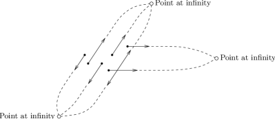
  Figure 1: Euclidean rays and lines passing through points at infinity in $\mathbb{T}_{2}$

• Travelling beyond these points at infinity, we add a second “hidden” copy of Euclidean $d$-space which we call invisible space; in contrast, we refer to our original copy of $\mathbb{E}_{d}$ as visible space. For computational purposes we can ignore invisible space—all of the Euclidean structures that we use in this paper will be situated in the visible copy of $\mathbb{E}_{d}$. Invisible space is simply a theoretical convenience that endows $\mathbb{T}_{d}$ with a number of useful geometric and analytical properties.

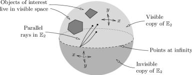
Figure 2: Building the oriented projective space $\mathbb{T}_{2}$

For illustration, Figure 2 shows the full construction of the oriented projective space $\mathbb{T}_{2}$. We see from this diagram that $\mathbb{T}_{2}$ has the topological structure of a sphere: the visible points lie on the northern hemisphere, the invisible points lie on the southern hemisphere, and the points at infinity lie on the equator. This picture generalises to higher dimensions, and Stolfi’s original construction shows how points in $\mathbb{T}_{d}$ correspond to points on the unit sphere in $\mathbb{R}^{d+1}$ via a geometric projection.

We coordinatise oriented projective $d$-space using signed homogeneous coordinates. Each point $\mathbf{p}\in\mathbb{T}_{d}$ is represented by a $(d+1)$-tuple of numbers, and two $(d+1)$-tuples $\mathbf{x},\mathbf{y}\in\mathbb{R}^{d+1}$ represent the same point of $\mathbb{T}_{d}$ if and only if $\mathbf{x}=\lambda\mathbf{y}$ for some scalar $\lambda>0$. So, for instance, the coordinates $(2,3,1)$, $(4,6,2)$ and $(1,\frac{3}{2},\frac{1}{2})$ all represent the same point of $\mathbb{T}_{2}$, but the coordinates $(-2,-3,-1)$ represent a different point. The coordinates $(0,\ldots,0)$ do not represent any point of $\mathbb{T}_{d}$ at all.

More specifically, we coordinatise the individual points of $\mathbb{T}_{d}$ as follows:

• Consider any Euclidean point $\mathbf{e}=(e_{1},\ldots,e_{d})\in\mathbb{E}_{d}$. In $\mathbb{T}_{d}$, the copy of $\mathbf{e}$ in visible space is described by the homogeneous coordinates $(\lambda e_{1},\ldots,\lambda e_{d},\lambda)$ for any $\lambda>0$, and the copy of $\mathbf{e}$ in invisible space is described by the homogeneous coordinates $(-\lambda e_{1},\ldots,-\lambda e_{d},-\lambda)$ for any $\lambda>0$.

• Consider any Euclidean ray $\{\mu\mathbf{r}\,|\,\mu\geq 0\}\subseteq\mathbb{E}_{d}$, where $\mathbf{r}=(r_{1},\ldots,r_{d})$. In $\mathbb{T}_{d}$, this ray in visible space extends to a point at infinity, which is described by the homogeneous coordinates $(r_{1},\ldots,r_{d},0)$.

Conversely, any point $\mathbf{x}\in\mathbb{T}_{d}$ with homogeneous coordinates $(x_{1},\ldots,x_{d+1})$ can be interpreted geometrically as follows:

• If $x_{d+1}>0$ then $\mathbf{x}$ describes the visible Euclidean point $(\frac{x_{1}}{x_{d+1}},\ldots,\frac{x_{d}}{x_{d+1}})\in\mathbb{E}_{d}$.

• If $x_{d+1}<0$ then $\mathbf{x}$ describes the invisible Euclidean point $(\frac{x_{1}}{x_{d+1}},\ldots,\frac{x_{d}}{x_{d+1}})\in\mathbb{E}_{d}$.

• If $x_{d+1}=0$ then $\mathbf{x}$ describes a point at infinity, which is the limiting point of the visible Euclidean ray $\{\mu\cdot(x_{1},\ldots,x_{d})\,|\,\mu\geq 0\}\subseteq\mathbb{E}_{d}$.

For brevity, we refer to such points as visible, invisible and infinite points of $\mathbb{T}_{d}$ respectively. Examples of all three types of point in $\mathbb{T}_{2}$ are illustrated in Figure 3.

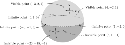
Figure 3: Different types of points in $\mathbb{T}_{2}$

A projective hyperplane in $\mathbb{T}_{d}$ is coordinatised by a $(d+1)$-tuple $\mathbf{h}=(h_{1},\ldots,h_{d+1})\in\mathbb{R}^{d+1}$, and contains all points $\mathbf{x}\in\mathbb{T}_{d}$ for which $h_{1}x_{1}+\ldots+h_{d+1}x_{d+1}=0$, or more concisely $\mathbf{h}\cdot\mathbf{x}=0$. Most projective hyperplanes consist of a Euclidean hyperplane in visible space and a Euclidean hyperplane in invisible space, joined together by a common set of points at infinity. The only exception is the infinite hyperplane described by the $(d+1)$-tuple $(0,\ldots,0,1)$, which contains all of the points at infinity and nothing else. Projective hyperplanes of both types are illustrated in Figure 4. The $(d+1)$-tuple $\lambda\mathbf{h}$ describes the same projective hyperplane as $\mathbf{h}$ for any $\lambda\neq 0$, and the $(d+1)$-tuple $(0,\ldots,0)$ does not describe any hyperplane at all.

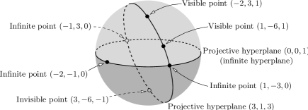
Figure 4: Two examples of projective hyperplanes in $\mathbb{T}_{2}$

A projective half-space in $\mathbb{T}_{d}$ is likewise coordinatised by a $(d+1)$-tuple $\mathbf{h}=(h_{1},\ldots,h_{d+1})\allowbreak\in\mathbb{R}^{d+1}$, and contains all points $\mathbf{x}\in\mathbb{T}_{d}$ for which $\mathbf{h}\cdot\mathbf{x}\geq 0$. Most projective half-spaces consist of a Euclidean half-space in visible space and a Euclidean half-space in invisible space, again joined together by a common set of points at infinity. There are two exceptions: the visible half-space described by the $(d+1)$-tuple $(0,\ldots,0,1)$ and the invisible half-space described by the $(d+1)$-tuple $(0,\ldots,0,-1)$. The visible half-space contains all visible and infinite points of $\mathbb{T}_{d}$, and the invisible half-space contains all invisible and infinite points of $\mathbb{T}_{d}$. All three types of projective half-space are illustrated in Figure 5. The $(d+1)$-tuple $\lambda\mathbf{h}$ describes the same projective half-space as $\mathbf{h}$ for any $\lambda>0$ (but not $\lambda<0$), and as usual $(0,\ldots,0)$ does not describe any half-space at all.

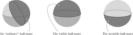
Figure 5: Different types of projective half-space in $\mathbb{T}_{2}$

For a projective half-space with coordinates $\mathbf{h}=(h_{1},\ldots,h_{d+1})$, the interior of this half-space consists of all points $\mathbf{x}\in\mathbb{T}_{d}$ for which $\mathbf{h}\cdot\mathbf{x}>0$; that is, all points of the half-space that do not lie on the boundary hyperplane. It is worth noting that the interior of the visible half-space is precisely the set of all visible Euclidean points.

For any point $\mathbf{x}\in\mathbb{T}_{d}$ with coordinates $(x_{1},\ldots,x_{d+1})$, the opposite point to $\mathbf{x}$ is the point with coordinates $(-x_{1},\ldots,-x_{d+1})$, which we denote $\neg\mathbf{x}$. The opposite of a visible point is an invisible point, and vice versa. If $\mathbf{x}$ is a point at infinity then $\neg\mathbf{x}$ is another point at infinity, and these points lie at opposite ends of the same Euclidean lines.

Arithmetic in $\mathbb{T}_{d}$ is very simple. For distinct and non-opposite points $\mathbf{x},\mathbf{y}\in\mathbb{T}_{d}$ with coordinates $(x_{1},\ldots,x_{d+1})$ and $(y_{1},\ldots,y_{d+1})$ respectively, the unique line joining $\mathbf{x}$ and $\mathbf{y}$ consists of all points with coordinates $(\alpha x_{1}+\beta y_{1},\ldots,\alpha x_{d+1}+\beta y_{d+1})$ for any $\alpha,\beta\in\mathbb{R}$, excluding the case $\alpha=\beta=0$. For the line segment joining $\mathbf{x}$ and $\mathbf{y}$ we add the constraints $\alpha,\beta\geq 0$. In other words, the arithmetic of lines in $\mathbb{T}_{d}$ is essentially the same as traditional Euclidean arithmetic in $\mathbb{R}^{d+1}$, except that we discard the constraint $\alpha+\beta=1$ (because signed homogeneous coordinates are unaffected by positive scaling).

We can define convexity in terms of line segments. Consider any set $S\subseteq\mathbb{T}_{d}$ that lies within the interior of some projective half-space. Then $S$ is convex if and only if, for any two points $\mathbf{x},\mathbf{y}\in S$, the entire line segment joining $\mathbf{x}$ and $\mathbf{y}$ lies within $S$. The half-space constraint ensures that $S$ cannot contain two opposite points, which means that line segments are always well-defined. Note that this half-space constraint is automatically satisfied for any set of visible Euclidean points (which all lie in the interior of the visible half-space).

Consider now some finite set of points $\mathbf{x}^{(1)},\ldots,\mathbf{x}^{(k)}\in\mathbb{T}_{d}$, where each $\mathbf{x}^{(i)}$ has coordinates $(x^{(i)}_{1},\ldots,x^{(i)}_{d+1})$, and again suppose that these points all lie within the interior of some projective half-space. The convex hull of these points is the smallest convex set containing all of $\mathbf{x}^{(1)},\ldots,\mathbf{x}^{(k)}$. Equivalently, it is the set of all points in $\mathbb{T}_{d}$ with coordinates of the form $(\sum\alpha_{i}x^{(i)}_{1},\ldots,\sum\alpha_{i}x^{(i)}_{d+1})$ for scalars $\alpha_{1},\ldots,\alpha_{i}\geq 0$, excluding the case $\alpha_{1}=\ldots=\alpha_{i}=0$.

It is important to note that, when we restrict our attention to visible Euclidean points, all of these concepts—lines, line segments, convexity and convex hulls—have precisely the same meaning as in traditional Euclidean geometry.

As noted earlier, the advantage of oriented projective geometry for us is the way in which it handles polytopes and polyhedra. Recall that in Euclidean geometry, a polyhedron (which may be bounded or unbounded) can be expressed as an intersection of finitely many half-spaces, and that a polytope (that is, a bounded polyhedron) can also be expressed as a convex hull of finitely many vertices. Using oriented projective geometry, we are able to express some unbounded polyhedra as convex hulls also. The details are as follows.

We define a projective polytope in $\mathbb{T}_{d}$ to be the convex hull of a finite set of points $V\subseteq\mathbb{T}_{d}$, all of which lie within the interior of some projective half-space. If the set $V$ is minimal (that is, no point can be removed from $V$ without changing the convex hull), we call the points of $V$ the vertices of the projective polytope.

It is clear that traditional Euclidean polytopes correspond precisely to projective polytopes whose vertices are all visible Euclidean points. The situation regarding unbounded Euclidean polyhedra is more interesting.

Suppose that the set $V\subseteq\mathbb{T}_{d}$ consists of a mixture of visible Euclidean points and points at infinity, and (as usual) that all of these points lie within the interior of some projective half-space. Then the projective polytope with vertex set $V$ is in fact an unbounded Euclidean polyhedron in visible space, “closed off” with additional points at infinity.

For example, Figure 6 shows a projective polytope in $\mathbb{T}_{2}$, with two visible vertices $(2,3,1)$ and $(3,2,1)$, and two infinite vertices $(-1,-1,0)$ and $(0,-1,0)$. The left-hand diagram shows this projective polytope in $\mathbb{T}_{2}$, and the right-hand diagram shows the corresponding unbounded polyhedron in $\mathbb{E}_{2}$.

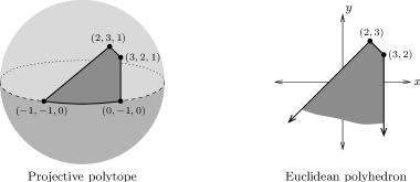
Figure 6: A 2-dimensional projective polytope with vertices at infinity

Conversely, let $P$ be an unbounded Euclidean polyhedron in $\mathbb{E}_{d}$ that lies within the interior of some Euclidean half-space. Then $P$ can be expressed as a projective polytope. More precisely, there is a projective polytope in $\mathbb{T}_{d}$ that consists of the polyhedron $P$ in visible space “closed off” with an extra facet at infinity. The vertices of this projective polytope are the vertices of $P$ in visible space with some additional vertices at infinity.

For a 3-dimensional example, Figure 7 shows a Euclidean polyhedron in $\mathbb{E}_{3}$ with vertices $(2,0,1)$, $(1,1,2)$ and $(0,2,0)$, and with facets that extend infinitely far in the negative $x$, $y$ and $z$ directions. The corresponding projective polytope has six vertices: the visible vertices $(2,0,1,1)$, $(1,1,2,1)$ and $(0,2,0,1)$, and the three infinite vertices $(-1,0,0,0)$, $(0,-1,0,0)$ and $(0,0,-1,0)$.

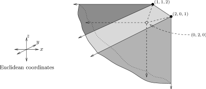
Figure 7: An unbounded 3-dimensional Euclidean polyhedron

As in traditional geometry, any projective polytope can be expressed as an intersection of finitely many projective half-spaces. Moreover, projective polytopes have the same combinatorial properties as Euclidean polytopes, and they support the same combinatorial algorithms (such as the double description method for vertex enumeration, which we use later in this paper).

4 Efficiency-equivalent polyhedra

Recall that our focus is on generating all efficient extreme outcomes for a multiobjective linear program. In other words, our aim is to generate all vertices of the outcome set $Y^{=}$ (a polytope in $\mathbb{E}_{p}$) that are also efficient (that is, not dominated by any other point in $Y^{=}$).

One difficulty is that the outcome set $Y^{=}$ can become extremely complex even for relatively small problems [36, 42], and the efficient vertices might only constitute a small fraction of the set of all vertices of $Y^{=}$. Several authors address this by working with efficiency-equivalent polyhedra—polyhedra in $\mathbb{E}_{p}$ that are typically simpler in structure than $Y^{=}$, but whose efficient sets precisely match the efficient outcome set $Y^{=}_{E}$.

There are two such polyhedra that feature prominently in the literature: the bounded polytope $Y^{\square}$ introduced by Benson [5], and the unbounded polyhedron $Y^{\leq}$ first described by Dauer and Saleh [12, 13], both of which we describe shortly. The goal of this section is to understand the structure and complexity of these two polyhedra.

We begin this section with a general result about efficiency-equivalent polyhedra that justifies our focus on vertices of these polyhedra. We then describe the efficiency-equivalent polyhedra $Y^{\square}$ and $Y^{\leq}$, and we reinterpret the unbounded polyhedron $Y^{\leq}$ as a polytope $T^{\leq}$ using oriented projective geometry. The remainder of this section concentrates on the complexity of the Euclidean polytope $Y^{\square}$ and the projective polytope $T^{\leq}$, paying particular attention to the number of “unwanted” non-efficient vertices. We find through our analysis that $T^{\leq}$ is far simpler than $Y^{\square}$ (and therefore far superior) in this respect.

4.1 Definitions and general results

Our first result shows that any efficiency-equivalent polyhedron for $Y^{=}$ can be used to generate the efficient extreme outcomes for our multiobjective linear program. Ours is a general result; Benson [5] and Dauer and Saleh [12] make similar observations for the specific polyhedra $Y^{\square}$ and $Y^{\leq}$ respectively.

Lemma 4.1.

Let $Z\subseteq\mathbb{E}_{p}$ be any efficiency-equivalent polyhedron for $Y^{=}$. Then the efficient vertices of $Z$ are precisely the efficient vertices of $Y^{=}$. That is, the efficient vertices of $Z$ are precisely the efficient extreme outcomes for our multiobjective linear program.

Proof.

Let $\mathbf{v}$ be an efficient vertex of $Y^{=}$. By efficiency-equivalence we know that $\mathbf{v}$ lies in the efficient set $Z_{E}$. We aim to show that $\mathbf{v}$ is a vertex (and thus an efficient vertex) of $Z$.

Let $F$ be the smallest-dimensional face of $Z$ containing $\mathbf{v}$. Because $Z_{E}$ is a union of faces of $Z$, every point in $F$ must be efficient. By efficiency-equivalence, the entire face $F$ must lie in $Y^{=}$ also. If $\mathbf{v}$ is not a vertex of $Z$ then $\mathbf{v}$ lies within the relative interior of the face $F$, and since $F\subseteq Y^{=}$ it follows that $\mathbf{v}$ cannot be a vertex of $Y^{=}$, a contradiction.

Applying the same argument in reverse shows that every efficient vertex of $Z$ is an efficient vertex of $Y^{=}$, and the proof is complete. ∎

We proceed now to define the polyhedra $Y^{\square}$ and $Y^{\leq}$, which will occupy our attention for the remainder of this section. Both are “extensions” of the outcome set $Y^{=}$, in that they enlarge the non-efficient portion of $Y^{=}$ to create a simpler structure.

Definition 4.2.

We define the Euclidean polyhedron $Y^{\leq}$ to be the set of all points in $\mathbb{E}_{p}$ that are dominated by any point in $Y^{=}$. That is,

$$Y^{\leq}=\left\{\mathbf{z}\in\mathbb{E}_{p}\,\left|\,\mathbf{z}\leq\mathbf{y}\ \textrm{for some}\ \mathbf{y}\in Y^{=}\right.\right\}.$$

Choose some point $\widehat{\mathbf{y}}\in\mathbb{E}_{p}$ that is strictly dominated by all of $Y^{=}$; in other words, $\widehat{\mathbf{y}}<\mathbf{y}$ for all $\mathbf{y}\in Y^{=}$. We then define the Euclidean polytope $Y^{\square}$ to be

$$Y^{\square}=\left\{\mathbf{z}\in\mathbb{E}_{p}\,\left|\,\widehat{\mathbf{y}}\leq\mathbf{z}\leq\mathbf{y}\ \textrm{for some}\ \mathbf{y}\in Y^{=}\right.\right\}.$$

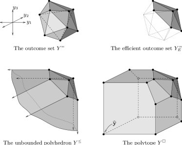
Figure 8: Constructing the efficiency-equivalent polyhedra $Y^{\leq}$ and $Y^{\square}$

Both of these structures are illustrated in Figure 8 (where we use $y_{1},y_{2},y_{3}$ for our three coordinate axes to show that we are working in objective space). It is clear that $Y^{\leq}$ is an unbounded polyhedron, and that it can be expressed as the Minkowski sum

$$Y^{\leq}=\left\{\mathbf{y}+\mathbf{z}\,\left|\,\mathbf{y}\in Y^{=}\ \mbox{and}\ \mathbf{z}\leq\mathbf{0}\right.\right\}.$$ (4.1)

Likewise, it is clear that $Y^{\square}$ is a polytope, since its points are bounded below by $\widehat{\mathbf{y}}$ and above by $Y^{=}$. Geometrically, $Y^{\square}$ truncates the unbounded polyhedron $Y^{\leq}$ by intersecting it with a large cube that surrounds the original outcome set $Y^{=}$.

The following crucial properties of $Y^{\square}$ and $Y^{\leq}$ are proven by Benson [5] and Dauer and Saleh [12] respectively.

Lemma 4.3.

Both $Y^{\square}$ and $Y^{\leq}$ are efficiency-equivalent polyhedra for $Y^{=}$. In other words, the efficient sets $Y^{\square}_{E}$, $Y^{\leq}_{E}$ and $Y^{=}_{E}$ are identical.

4.2 The complexity of $Y^{\leq}$ and $T^{\leq}$

The unbounded polytope $Y^{\leq}$ is simpler than $Y^{\square}$ in structure, with fewer vertices and a convenient Minkowski sum representation. However, $Y^{\leq}$ is more difficult to work with algorithmically because it is not a polytope—in particular, it cannot be expressed as the convex hull of its vertices. This makes it less amenable to traditional algorithms for vertex enumeration and linear optimisation.

We now grant ourselves the best of both worlds by reinterpreting the unbounded polyhedron $Y^{\leq}$ as a convex hull of vertices in oriented projective $p$-space.

Definition 4.4.

Let $T^{\leq}$ be the projective polytope in $\mathbb{T}_{p}$ formed as the convex hull of:

1. the vertices of the polyhedron $Y^{\leq}$ in visible Euclidean space;

2. the points at infinity defined by the signed homogeneous coordinates $(-1,0,0,\ldots,0,0)$, $(0,-1,0,\ldots,0,0)$, $(0,0,-1,\ldots,0,0)$, …, $(0,0,0,\ldots,-1,0)$ (there are $p$ such points in total).

In the following series of results, we show that the projective polytope $T^{\leq}$ is well-defined, that it is truly a projective reinterpretation of $Y^{\leq}$, and that Definition 4.4 gives the precise vertex structure of $T^{\leq}$ in oriented projective $p$-space.

Lemma 4.5.

The projective polytope $T^{\leq}$ is well-defined. That is, all of the points listed in (i) and (ii) above lie in the interior of some projective half-space.

Proof.

Because the Euclidean polyhedron $Y^{\leq}$ has finitely many vertices, there is some $\alpha\in\mathbb{R}$ that satisfies $\alpha>v_{1}+\ldots+v_{p}$ for every Euclidean vertex $(v_{1},\ldots,v_{p})$ of $Y^{\leq}$. When translated into oriented projective $p$-space, it follows that every vertex of $Y^{\leq}$ lies in the interior of the projective half-space with signed homogeneous coordinates $(-1,\ldots,-1,\alpha)$. The same is clearly true for each infinite point in list (ii) above, and so the projective half-space $(-1,\ldots,-1,\alpha)$ is the half-space that we seek. ∎

Lemma 4.6.

The visible portion of the projective polytope $T^{\leq}$ is precisely the Euclidean polyhedron $Y^{\leq}$.

Proof.

We prove this by first showing that every visible Euclidean point of $T^{\leq}$ belongs to $Y^{\leq}$, and then that every point of the visible Euclidean polyhedron $Y^{\leq}$ belongs to $T^{\leq}$.

• Let $\mathbf{t}\in\mathbb{T}_{p}$ be some visible Euclidean point in $T^{\leq}$. We first observe that any convex combination of points in list (i) above is a visible Euclidean point in $Y^{\leq}$, and that any convex combination of points in list (ii) above is a point at infinity with signed homogeneous coordinates $(-\beta_{1},\ldots,-\beta_{p},0)$ for some scalars $\beta_{1},\ldots,\beta_{p}\geq 0$. Since $\mathbf{t}$ is a convex combination of points in both lists, it follows that $\mathbf{t}$ has signed homogeneous coordinates of the form $(\mu y_{1}-\lambda\beta_{1},\ldots,\mu y_{p}-\lambda\beta_{p},\mu)$, where $\mu,\lambda,\beta_{1},\ldots,\beta_{p}\geq 0$ and where $(y_{1},\ldots,y_{p})$ are the Euclidean coordinates of some point in $Y^{\leq}$.

  Because $\mathbf{t}$ is visible we must have $\mu>0$, so we can rescale the coordinates of $\mathbf{t}$ to $(y_{1}-\lambda\beta_{1}/\mu,\ldots,y_{p}-\lambda\beta_{p}/\mu,1)$. It is clear then that $\mathbf{t}$ is a visible point whose Euclidean coordinates are formed by adding the non-positive vector $-\lambda/\mu(\beta_{1},\ldots,\beta_{p})$ to some point in $Y^{\leq}$. From equation (4.1) it follows that $\mathbf{t}$ is a visible Euclidean point in $Y^{\leq}$.

• Now let $\mathbf{y}\in\mathbb{T}_{p}$ be a point of $Y^{\leq}$ in visible Euclidean space with signed homogeneous coordinates $(y_{1},\ldots,y_{p},1)$. Let $\mathbf{z}=(z_{1},\ldots,z_{p},1)$ be an efficient point of $Y^{\leq}$ that dominates $\mathbf{y}$. We can express the coordinates of $\mathbf{y}$ as $(z_{1}-\beta_{1},\ldots,z_{p}-\beta_{p},1)$ for some scalars $\beta_{1},\ldots,\beta_{p}\geq 0$, which shows that $\mathbf{y}$ is a convex combination of the efficient point $\mathbf{z}$ with the points at infinity in list (ii) above.

  Recalling that the efficient set $Y^{\leq}_{E}$ is a union of faces of $Y^{\leq}$, let $F$ be some efficient face of $Y^{\leq}$ containing $\mathbf{z}$. Because $Y^{\leq}$ is efficiency-equivalent to the bounded polytope $Y^{=}$, the efficient face $F$ must likewise be bounded. Therefore $\mathbf{z}$ can be expressed as a convex combination of vertices of $F$, which are of course vertices of $Y^{\leq}$ also. This allows us to express $\mathbf{y}$ as a convex combination of points in lists (i) and (ii), and so $\mathbf{y}$ belongs to the projective polytope $T^{\leq}$. ∎

Lemma 4.7.

The vertices of $T^{\leq}$ are precisely the points listed in Definition 4.4. In other words, no point can be removed from these lists without changing the convex hull.

Proof.

To prove this we must show that no point in lists (i) and (ii) from Definition 4.4 can be expressed as a convex combination of the others. Suppose that list (i) contains the points $\mathbf{v}_{1},\ldots,\mathbf{v}_{t}$ (these are the vertices of $Y^{\leq}$), and that list (ii) contains the points $\mathbf{f}_{1},\ldots,\mathbf{f}_{p}$ (these are all points at infinity).

• No $\mathbf{f}_{i}$ can be expressed as a convex combination of the other points in these lists, since each other point introduces some non-zero coordinate that is zero in $\mathbf{f}_{i}$.

• Suppose that some $\mathbf{v}_{i}$ can be expressed as the convex combination $\sum_{j\neq i}\alpha_{j}\mathbf{v}_{j}+\sum_{k}\gamma_{k}\mathbf{f}_{k}$ where each $\alpha_{j},\gamma_{k}\geq 0$ (as usual we work in homogeneous coordinates). Some $\alpha_{j}$ must be non-zero, since otherwise $\mathbf{v}_{i}$ would be a point at infinity. Some $\gamma_{k}$ must also be non-zero, since we cannot express a vertex of $Y^{\leq}$ as a convex combination of other vertices.

  It follows that we can express $\mathbf{v}_{i}$ in the form $(y_{1}-\beta_{1},\ldots,y_{p}-\beta_{p},1)$, where $\mathbf{y}=(y_{1},\ldots,y_{p},1)$ is a convex combination of vertices of $Y^{\leq}$ (in particular, $\mathbf{y}\in Y^{\leq}$), and where $\beta_{1},\ldots,\beta_{p}\geq 0$ with at least one $\beta_{k}$ strictly positive. This places $\mathbf{v}_{i}$ in the interior of the line segment joining $\mathbf{y}$ with the point $(y_{1}-2\beta_{1},\ldots,y_{p}-2\beta_{p},1)$. However, both endpoints of this line segment lie in the polyhedron $Y^{\leq}$, which is impossible since $\mathbf{v}_{i}$ is a vertex of $Y^{\leq}$. ∎

We can draw some important conclusions from these results. The first is that $T^{\leq}$ is precisely the efficiency-equivalent polyhedron $Y^{\leq}$, recast as a polytope using oriented projective geometry. Furthermore, Lemma 4.7 gives an insight into the complexity of this polytope, as seen in the following result.

Corollary 4.8.

The visible Euclidean vertices of $T^{\leq}$ are precisely the efficient extreme outcomes for our multiobjective linear program. That is, the only vertices of $T^{\leq}$ that are not efficient extreme outcomes are the $p$ vertices at infinity.

Proof.

From Lemma 4.7, the visible Euclidean vertices of $T^{\leq}$ are precisely the vertices of the unbounded polyhedron $Y^{\leq}\subseteq\mathbb{E}_{p}$. Moreover, Lemma 4.1 shows that the efficient vertices of $Y^{\leq}$ are precisely the efficient extreme outcomes.

Suppose that $Y^{\leq}$ has some non-efficient vertex $\mathbf{v}\in Y^{\leq}$. Then $\mathbf{v}$ must be dominated by some other point $\mathbf{x}\in Y^{\leq}$, so that the difference $\mathbf{d}=\mathbf{x}-\mathbf{v}$ is non-negative and non-zero. Now construct the point $\mathbf{x}^{\prime}=\mathbf{v}-\mathbf{d}$. It is clear that $\mathbf{x}^{\prime}\in Y^{\leq}$ and that $\mathbf{v}$ lies strictly inside the line segment $[\mathbf{x},\mathbf{x}^{\prime}]\subseteq Y^{\leq}$, contradicting the claim that $\mathbf{v}$ is a vertex of $Y^{\leq}$. ∎

It follows from Corollary 4.8 that the projective polytope $T^{\leq}$ gives an extremely compact representation of the efficient extreme outcomes—the number of additional “unwanted” vertices grows linearly with the number of objectives $p$, and does not depend at all on the problem size $(n,m)$.

4.3 The complexity of $Y^{\square}$

We turn now to study the complexity of the Euclidean polytope $Y^{\square}$. We begin with a complete categorisation of vertices of $Y^{\square}$, and we follow with a discussion of what this means for best-case and worst-case complexity. Throughout the remainder of this section we work entirely in Euclidean coordinates.

Definition 4.9.

For each set of indices $S\subseteq\{1,\ldots,p\}$, we define the set of points $V(S)\subseteq\mathbb{E}_{p}$ as follows. Denote the $p$ objectives by $y_{1},\ldots,y_{p}$, and consider the smaller multiobjective linear program obtained by considering only the objectives $\{y_{i}\,|\,i\in S\}$ (in other words, by deleting the $i$th row of the objective matrix for each $i\notin S$). This smaller problem yields a smaller set of efficient extreme outcomes in the space $\mathbb{E}_{|S|}$.

We extend these efficient extreme outcomes to points in $\mathbb{E}_{p}$ as follows. For each deleted objective $i\notin S$, we fix the coordinate $y_{i}$ to the value $\widehat{y}_{i}$ (using the point $\widehat{\mathbf{y}}\in\mathbb{E}_{p}$ that we describe in Definition 4.2). The resulting set of points in $\mathbb{E}_{p}$ is denoted $V(S)$.

If $S$ is the empty set then there is no linear program to solve, and we simply define $V(\emptyset)=\{\widehat{\mathbf{y}}\}$.

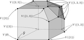
Figure 9: The sets $V(S)$ in relation to the polytope $Y^{\square}$

It is worth noting that for the full set $S=\{1,\ldots,p\}$, the points in $V(S)$ are simply the efficient extreme outcomes for our original (full-dimensional) multiobjective linear program.

The various sets $V(S)$ are illustrated in Figure 9, which continues the earlier example of Figure 8. We see in this diagram that the sets $V(S)$ together describe all of the vertices of $Y^{\square}$. This is no accident, as shown by the following result.

Theorem 4.10.

The sets $V(S)$ are pairwise disjoint; that is, if $S\neq S^{\prime}$ then $V(S)\cap V(S^{\prime})=\emptyset$. Moreover, the union of all such sets $V(S)$ over all $S\subseteq\{1,\ldots,p\}$ gives the complete vertex set for the polytope $Y^{\square}$.

Proof.

Pairwise disjointness is simple to prove. Because $\widehat{\mathbf{y}}$ is strictly dominated by all $\mathbf{y}\in Y^{=}$, we find that for any $\mathbf{v}=(v_{1},\ldots,v_{p})\in V(S)$ we have $v_{i}=\widehat{y}_{i}$ if and only if $i\in S$. It is then clear that $\mathbf{v}$ cannot belong to both $V(S)$ and $V(S^{\prime})$ for distinct sets $S\neq S^{\prime}$.

It remains to show that every element of each set $V(S)$ is a vertex of $Y^{\square}$, and that every vertex of $Y^{\square}$ can be expressed as an element of some $V(S)$. For this it is convenient to define the linear projection $\pi_{S}\colon\thinspace\mathbb{E}_{p}\to\mathbb{E}_{|S|}$ that simply deletes all coordinates $y_{i}$ for $i\notin S$. For example, if $S=\{1,\ldots,p\}$ then $\pi_{S}$ is the identity map, and if $S=\{i\}$ then $\pi_{S}$ merely extracts the $i$th coordinate.

From Definition 4.9 we have $\mathbf{v}\in V(S)$ if and only if (i) $v_{i}=\widehat{y}_{i}$ for each $i\notin S$, and (ii) the projection $\pi_{S}(\mathbf{v})$ is an efficient vertex of the polytope $\pi_{S}(Y^{=})$. However, applying Lemma 4.3 to the smaller multiobjective linear program with objectives $\{y_{i}\,|\,i\in S\}$ shows that $\pi_{S}(Y^{\square})$ is efficiency-equivalent to $\pi_{S}(Y^{=})$. This means that $\mathbf{v}\in V(S)$ if and only if (i) $v_{i}=\widehat{y}_{i}$ for each $i\notin S$, and ($\mathrm{ii}^{\prime}$) $\pi_{S}(\mathbf{v})$ is an efficient vertex of $\pi_{S}(Y^{\square})$.

We can now conclude the proof as follows:

• Suppose that $\mathbf{v}\in V(S)$ for some set $S\neq\emptyset$. We aim to show that $\mathbf{v}$ is a vertex of $Y^{\square}$. If not, we can express $\mathbf{v}=\frac{1}{2}(\mathbf{u}+\mathbf{w})$ for some distinct $\mathbf{u},\mathbf{w}\in Y^{\square}$. We proceed to derive a contradiction by showing that $\mathbf{v}=\mathbf{u}=\mathbf{w}$.

  • For any $i\notin S$ we have $v_{i}=\widehat{y}_{i}$ by definition of $V(S)$, and $u_{i},w_{i}\geq\widehat{y}_{i}$ by definition of $Y^{\square}$. Since $\mathbf{v}=\frac{1}{2}(\mathbf{u}+\mathbf{w})$ it follows that $v_{i}=u_{i}=w_{i}$.

  • By linearity, $\pi_{S}(\mathbf{v})=\frac{1}{2}\left(\pi_{S}(\mathbf{u})+\pi_{S}(\mathbf{w})\right)$ where $\pi_{S}(\mathbf{u}),\pi_{S}(\mathbf{w})\in\pi_{S}(Y^{\square})$. However, because $\mathbf{v}\in V(S)$ we know that $\pi_{S}(\mathbf{v})$ is a vertex of $\pi_{S}(Y^{\square})$, which is only possible if $\pi_{S}(\mathbf{v})=\pi_{S}(\mathbf{u})=\pi_{S}(\mathbf{w})$. That is, $v_{i}=u_{i}=w_{i}$ for all $i\in S$.

  This establishes $\mathbf{v}=\mathbf{u}=\mathbf{w}$, and we conclude that $\mathbf{v}$ must indeed be a vertex of $Y^{\square}$.

  We handle the case $S=\emptyset$ by observing that $V(\emptyset)$ contains the single point $\widehat{\mathbf{y}}$, and that $\widehat{\mathbf{y}}$ is a vertex of $Y^{\square}$ because it uniquely minimises the linear functional $\mathbf{y}\mapsto y_{1}+\ldots+y_{p}$.

• Now let $\mathbf{v}$ be some vertex of $Y^{\square}$, and let $S=\{i\,|\,v_{i}\neq\widehat{y}_{i}\}$. We aim to show that $\mathbf{v}\in V(S)$. If $S=\emptyset$ then $\mathbf{v}=\widehat{\mathbf{y}}\in V(\emptyset)$, so assume that $S$ is non-empty. We already have $v_{i}=\widehat{y}_{i}$ for each $i\notin S$, so we only need to show that $\pi_{S}(\mathbf{v})$ is an efficient vertex of $\pi_{S}(Y^{\square})$.

  • If $\pi_{S}(\mathbf{v})$ is not a vertex of $\pi_{S}(Y^{\square})$, there must be some $\mathbf{u},\mathbf{w}\in Y^{\square}$ for which $\pi_{S}(\mathbf{v})=\frac{1}{2}\left(\pi_{S}(\mathbf{u})+\pi_{S}(\mathbf{w})\right)$ but $\pi_{S}(\mathbf{u})\neq\pi_{S}(\mathbf{w})$. Construct the points $\mathbf{u}^{\prime},\mathbf{w}^{\prime}$ from $\mathbf{u},\mathbf{w}$ respectively by replacing each $i$th coordinate with $\widehat{y}_{i}$ for all $i\notin S$.

    It is clear that $\mathbf{u}^{\prime},\mathbf{w}^{\prime}\in Y^{\square}$ (since $\widehat{\mathbf{y}}\leq\mathbf{u}^{\prime}\leq\mathbf{u}$ and $\widehat{\mathbf{y}}\leq\mathbf{w}^{\prime}\leq\mathbf{w}$). Moreover, for $i\notin S$ we have $v_{i}=u^{\prime}_{i}=w^{\prime}_{i}$, and for $i\in S$ we have $v_{i}=\frac{1}{2}(u^{\prime}_{i}+w^{\prime}_{i})$. Finally, we note that $\pi_{S}(\mathbf{u})\neq\pi_{S}(\mathbf{w})$ implies that $\mathbf{u}^{\prime}\neq\mathbf{w}^{\prime}$. We therefore have $\mathbf{v}=\frac{1}{2}(\mathbf{u^{\prime}}+\mathbf{w^{\prime}})$ but $\mathbf{u^{\prime}}\neq\mathbf{w^{\prime}}$, contradicting the assumption that $\mathbf{v}$ is a vertex of $Y^{\square}$.

  • If $\pi_{S}(\mathbf{v})$ is not efficient in $\pi_{S}(Y^{\square})$, there must be some $\mathbf{u}\in Y^{\square}$ for which $\pi_{S}(\mathbf{u})\geq\pi_{S}(\mathbf{v})$ but $\pi_{S}(\mathbf{u})\neq\pi_{S}(\mathbf{v})$. Again, construct $\mathbf{u}^{\prime}$ from $\mathbf{u}$ by replacing the $i$th coordinate with $\widehat{y}_{i}$ for each $i\notin S$. This time we have $\mathbf{u}^{\prime}\in Y^{\square}$, $\mathbf{u}^{\prime}\neq\mathbf{v}$, and the relations $\widehat{y}_{i}=v_{i}=u^{\prime}_{i}$ for $i\notin S$ and $\widehat{y}_{i}<v_{i}\leq u^{\prime}_{i}$ for $i\in S$.

    Let $\mathbf{z}=\mathbf{v}-\varepsilon(\mathbf{u}^{\prime}-\mathbf{v})$ for some small $\varepsilon>0$ that ensures $\widehat{\mathbf{y}}\leq\mathbf{z}$ (by the relations above, such an $\varepsilon$ exists). Then $\mathbf{z}\in Y^{\square}$ and $\mathbf{v}$ is in the interior of the line segment $[\mathbf{z},\mathbf{u}^{\prime}]$, again contradicting the assumption that $\mathbf{v}$ is a vertex of $Y^{\square}$.

  Together these observations show that $\pi_{S}(\mathbf{v})$ is an efficient vertex of $\pi_{S}(Y^{\square})$, whereupon the proof is complete. ∎

Theorem 4.10 has important implications for the complexity of the polytope $Y^{\square}$. Recall that all of the efficient vertices of $Y^{\square}$ are held in the single set $V(\{1,\ldots,p\})$. This means that for every proper subset $S\subset\{1,\ldots,p\}$, the corresponding $V(S)$ is filled with non-efficient vertices of $Y^{\square}$. This can yield an extremely large number of non-efficient vertices—each $V(S)$ describes the efficient extreme outcomes for some other multiobjective linear program with up to $p-1$ objectives, and we already know that the number of such outcomes can grow very large even for relatively small values of $p$, $n$ and $m$ [36, 42].

This argument shows intuitively that $Y^{\square}$ can have an extremely large number of non-efficient vertices. We follow now with two corollaries of Theorem 4.10 that back this up with explicit formulae. The first result shows that, even in the best case scenario where $Y^{\square}$ is as simple as possible, we still obtain an exponentially large number of non-efficient vertices.

Corollary 4.11.

The polytope $Y^{\square}$ always has at least $2^{p}-1$ non-efficient vertices; that is, $2^{p}-1$ vertices that are not efficient extreme outcomes for our original multiobjective linear program.

Proof.

As noted above, every proper subset $S\subset\{1,\ldots,p\}$ yields a corresponding $V(S)$ that consists entirely of non-efficient vertices. There are $2^{p}-1$ proper subsets of $\{1,\ldots,p\}$, and so we have at least $2^{p}-1$ non-efficient vertices in total. ∎

The corollary above shows that the growth rate of non-efficient vertices relative to the number of objectives $p$ is unavoidably exponential. In our second corollary, we show that the number of non-efficient vertices can also grow at a severe rate relative to the problem size $(n,m)$. This is an asymptotic result, and we use the standard notation for complexity whereby $O(\cdot)$ and $\Omega(\cdot)$ denote asymptotic upper bounds and lower bounds respectively.

Corollary 4.12.

Suppose we fix $p$ and allow the problem size $(n,m)$ to vary. Then there are multiobjective linear programs for which the number of non-efficient vertices of $Y^{\square}$ grows at least as fast as $\Omega(n^{\lfloor(p-1)/2\rfloor})$.

Proof.

We establish this result using dual cyclic polytopes. For any integers $2\leq d<k$, the $(d,k)$ dual cyclic polytope is a $d$-dimensional polytope with precisely $k$ facets and

$$\binom{k-\lfloor\frac{d+1}{2}\rfloor}{k-d}+\binom{k-\lfloor\frac{d+2}{2}\rfloor}{k-d}$$ (4.2)

vertices. For further information on dual cyclic polytopes the reader is referred to a standard reference such as Grünbaum [22].

For us, the important fact about dual cyclic polytopes is that for a fixed dimension $d$, the number of vertices grows at least as fast as $\Omega(k^{\lfloor d/2\rfloor})$. This is because the sum of binomial coefficients in equation (4.2) can be rewritten as a $\lfloor d/2\rfloor$-degree polynomial in $k$ (taking separate cases for odd and even $d$).

Our strategy then is as follows. Suppose we are given some number of objectives $p$ and some number of variables $n$. We assume here that $3\leq p\leq n$ (since we are interested in the growth rate as $n$ becomes large, and for $p\leq 2$ the result is trivial). Let $H$ be the hyperplane in $\mathbb{E}_{p}$ defined by the equation $y_{1}+\ldots+y_{p}=1$. We now embed a $(p-1,n)$ dual cyclic polytope $P$ within the hyperplane $H$ (a straightforward procedure since $\dim H=p-1$).

The polytope $P\subseteq\mathbb{E}_{p}$ can be expressed as the outcome set $Y^{=}$ for some multiobjective linear program with $p$ objectives and $n$ variables (its $n$ facets arise from the inequalities $\mathbf{x}\geq 0$ in the solution space $\mathbb{E}_{n}$). Although $P$ is not full-dimensional in $\mathbb{E}_{p}$, this is just a convenience to keep our arithmetic simple. If a full-dimensional example is ever required then we simply extend $P$ to a $p$-dimensional cone; the analysis becomes messier but the final growth rate of $\Omega(n^{\lfloor(p-1)/2\rfloor})$ remains the same.

We can now make the following observation.

Claim: Every vertex of $Y^{=}$ (that is, $P$) gives an efficient extreme outcome for some smaller multiobjective linear program that uses only $p-1$ of our $p$ objectives.

We will prove this claim shortly. In the meantime, we examine its consequences. By Theorem 4.10, it follows that each vertex of $P$ corresponds to some element of $V(S)$ where $S$ is some $(p-1)$-element subset of $\{1,\ldots,p\}$. Moreover, because $P$ lies entirely within the hyperplane $\sum y_{i}=1$, any two vertices of $P$ must differ in at least two coordinates. It follows that any two distinct vertices of $P$ must correspond to either two distinct elements of the same set $V(S)$, or else elements of two distinct sets $V(S)$, $V(S^{\prime})$.

As a result, the sum of $|V(S)|$ over all $(p-1)$-element sets $S$ is at least the number of vertices of $P$. However, each such $S$ is a proper subset of $\{1,\ldots,p\}$, and we can therefore deduce that the total number of non-efficient vertices of $Y^{\square}$ is at least the number of vertices of $P$. The number of vertices of $P$ is described by equation (4.2), which we noted earlier grows at least as fast as $\Omega(k^{\lfloor d/2\rfloor})=\Omega(n^{\lfloor(p-1)/2\rfloor})$. Thus our final result is established.

All that remains then is to prove the claim above. Let $\mathbf{v}$ be any vertex of $Y^{=}$. It follows that $\mathbf{v}$ is the unique intersection of $Y^{=}$ with some supporting hyperplane $H\subseteq\mathbb{E}_{p}$. Suppose that $H$ is defined by the equation $\alpha_{1}y_{1}+\ldots+\alpha_{p}y_{p}=0$, where $Y^{=}$ lies in the closed half-space $\alpha_{1}y_{1}+\ldots+\alpha_{p}y_{p}\leq 0$.

We can “tilt” this hyperplane as follows. Let $\alpha_{\mathrm{min}}=\min\{\alpha_{i}\}$, and consider instead the hyperplane $H^{\prime}\subseteq\mathbb{E}_{p}$ defined by the equation $(\alpha_{1}-\alpha_{\mathrm{min}})y_{1}+\ldots+(\alpha_{p}-\alpha_{\mathrm{min}})y_{p}=0$. Because every point in $Y^{=}$ satisfies $\sum y_{i}=1$, we find that $H^{\prime}$ is also a supporting hyperplane for $Y^{=}$, that $Y^{=}$ lies in the closed half-space $(\alpha_{1}-\alpha_{\mathrm{min}})y_{1}+\ldots+(\alpha_{p}-\alpha_{\mathrm{min}})y_{p}\leq 0$, and that $\mathbf{v}$ is the unique intersection of $Y^{=}$ with $H^{\prime}$.

More importantly, at least one of the coefficients $(\alpha_{i}-\alpha_{\mathrm{min}})$ is zero, and all of the remaining coefficients of $H^{\prime}$ are non-negative. It follows that $(\alpha_{1}-\alpha_{\mathrm{min}})y_{1}+\ldots+(\alpha_{p}-\alpha_{\mathrm{min}})y_{p}$ is a linear functional with non-negative coefficients in at most $p-1$ objectives, and that $\mathbf{v}$ is the unique maximum for this linear functional in the outcome set $Y^{=}$. As a result, $\mathbf{v}$ indeed gives an efficient extreme outcome for some smaller multiobjective linear program using only $p-1$ of our $p$ objectives. ∎

5 The outer approximation algorithm

In this section we illustrate the power of our techniques by applying them to the outer approximation algorithm, which enumerates efficient extreme outcomes for a multiobjective linear program. Introduced by Benson [5], this algorithm iteratively constructs the efficiency-equivalent polytope $Y^{\square}$ using methods from linear programming, univariate search techniques and polytope vertex enumeration algorithms. The algorithm is designed to work with polytopes, not unbounded polyhedra, which explains the choice of $Y^{\square}$ as the final target.

We begin in Section 5.1 by describing the original outer approximation algorithm in detail. In Section 5.2 we develop a new outer approximation algorithm by working in oriented projective geometry, which allows us to replace the target polytope $Y^{\square}$ with the much simpler projective polytope $T^{\leq}$. In Section 5.3 we examine how these changes affect the runtime complexity.

5.1 The original algorithm

The algorithm originally described by Benson begins with a simplex in $\mathbb{E}_{p}$ that completely surrounds the outcome set $Y^{=}$, and then successively truncates this simplex along hyperplanes until it is eventually whittled down to the target polytope $Y^{\square}$. This overall procedure is illustrated in Figure 10 (which continues the earlier example from Figure 8). The details are as follows.

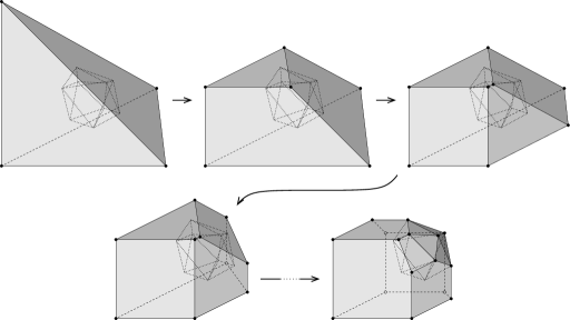
Figure 10: Stepping through the original outer approximation algorithm

Algorithm 5.1 (Outer approximation algorithm).

This algorithm builds $Y^{\square}$ by constructing a series of polytopes $P_{0}\supseteq P_{1}\supseteq\ldots\supseteq P_{k}=Y^{\square}$ in $\mathbb{E}_{p}$ (where the number of polytopes $k$ is not known in advance). Each polytope is stored using two representations: as a convex hull of vertices in $\mathbb{E}_{p}$, and as an intersection of half-spaces in $\mathbb{E}_{p}$.

To initialise the algorithm, choose an arbitrary point $\overline{\mathbf{y}}$ in the interior of $Y^{\square}$, and set the initial polytope $P_{0}$ to be a simplex with vertex set $\{\widehat{\mathbf{y}}$, $\widehat{\mathbf{y}}+\alpha\mathbf{e}_{1}$, …, $\widehat{\mathbf{y}}+\alpha\mathbf{e}_{p}\}$. Here $\widehat{\mathbf{y}}$ is the point chosen in Definition 4.2, each $\mathbf{e}_{i}$ represents the $i$th unit vector in $\mathbb{E}_{p}$, and the constant $\alpha$ is chosen so that the simplex contains the entire outcome set $Y^{=}$.

Now iteratively construct each polytope $P_{i+1}$ from the previous polytope $P_{i}$ as follows:

1. Search through the vertices of $P_{i}$ for one that does not belong to the target polytope $Y^{\square}$. If no such vertex exists (which indicates that $P_{i}=Y^{\square}$), then output the efficient vertices of $P_{i}$ and terminate the algorithm.

2. Otherwise let $\mathbf{v}$ be such a vertex, and compute the unique point $\mathbf{x}\in\mathbb{E}_{p}$ at which the line segment joining $\mathbf{v}$ with $\overline{\mathbf{y}}$ crosses the boundary of the target polytope $Y^{\square}$.

3. Compute a half-space $H\subseteq\mathbb{E}_{p}$ that contains the target polytope $Y^{\square}$, and that has the point $\mathbf{x}$ in its bounding hyperplane.

4. The next polytope is now $P_{i+1}=P_{i}\cap H$. Compute a half-space representation of $P_{i+1}$ (which is trivial) and a convex hull representation (which is not).

There are significant details to be filled in for each of these steps, for which we refer the reader to Benson’s original paper [5]. In brief:

• In the initialisation phase, both the constant $\alpha$ and the interior point $\overline{\mathbf{y}}\in Y^{\square}$ can be found by solving a linear program, and the half-space representation of the initial simplex $P_{0}$ is then simple to compute.

• In Step 1 of the iteration, we can test for membership in $Y^{\square}$ by testing the feasibility of another linear program. The boundary point $\mathbf{x}$ in Step 2 is found by combining feasibility tests with standard univariate search techniques (Benson uses a simple bisection search), and the half-space $H$ in Step 3 uses the solution to a dual linear program.

• In the final output phase, the efficient vertices of $P_{i}=Y^{\square}$ are precisely those vertices that are strictly dominated by $\widehat{\mathbf{y}}$.

The only step not covered in the list above is Step 4, which requires us to compute half-space and convex hull representations for the new polytope $P_{i+1}$. The half-space representation is simple: just append $H$ to the list of half-spaces for the previous polytope $P_{i}$. The convex hull representation is more complex, and requires iterative vertex enumeration techniques. These are typically based on the double description method of Motzkin et al. [29], though the central idea has been rediscovered by many different authors and goes under a variety of names. See Chen et al. [9] and Horst et al. [23] for alternative treatments.

The fundamental principle behind the double description method is the following result:

Theorem 5.2.

Let $P\subseteq\mathbb{E}_{p}$ be a polytope, and let $H\subseteq\mathbb{E}_{p}$ be a half-space. Then the vertices of the polytope $P\cap H$ can be obtained from the vertices of $P$ using the following procedure.

First partition the vertices of $P$ into three sets $S_{+}$, $S_{0}$ and $S_{-}$, according to whether each vertex lies within the interior of $H$, on the bounding hyperplane of $H$, or external to $H$ respectively.

Each vertex in $S_{0}$ or $S_{+}$ then becomes a vertex of $P\cap H$. Furthermore, for each pair of vertices $\mathbf{u}\in S_{+}$ and $\mathbf{v}\in S_{-}$ that are adjacent in $P$, the point where the line segment $[\mathbf{u},\mathbf{v}]$ cuts the bounding hyperplane of $H$ also becomes a vertex of $P\cap H$. The polytope $P\cap H$ has no other vertices besides those described here.

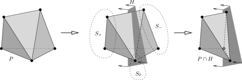
Figure 11: Intersecting the polytope $P$ with the half-space $H$

This procedure is illustrated in Figure 11. The only complication of Theorem 5.2 is determining which pairs of vertices $\mathbf{u}\in S_{+}$ and $\mathbf{v}\in S_{-}$ are adjacent (i.e., joined by an edge) in the original polytope $P$. There are many different adjacency tests in the literature; in this paper we use the combinatorial adjacency test, which is found to be fast and simple in practice [18], and which translates well to the setting of oriented projective geometry (as seen later in Theorem 5.6).

Lemma 5.3.

Let $P\subseteq\mathbb{E}_{p}$ be a polytope with half-space representation $P=H_{1}\cap H_{2}\cap\ldots\cap H_{k}$, where each $H_{k}$ is a half-space in $\mathbb{E}_{p}$. Then two vertices $\mathbf{u},\mathbf{v}$ of $P$ are adjacent if and only if there is no other vertex $\mathbf{z}$ of $P$ with the following property:

• For each half-space $H_{i}$, if both $\mathbf{u}$ and $\mathbf{v}$ lie on the bounding hyperplane of $H_{i}$ then $\mathbf{z}$ lies on the bounding hyperplane also.

For proofs of Theorem 5.2 and Lemma 5.3 as well as further details on the double description method, the reader is referred to Fukuda and Prodon [18].

5.2 A new algorithm

We now apply the results of Section 4 to the outer approximation algorithm, yielding a new algorithm with significant benefits over the original. Our strategy is to work in the oriented projective space $\mathbb{T}_{p}$ instead of the Euclidean space $\mathbb{E}_{p}$. This allows us to iteratively construct the projective polytope $T^{\leq}$ instead of the Euclidean polytope $Y^{\square}$, thereby removing an exponential number of non-efficient vertices that would otherwise clutter up our computations. We discuss the running time benefits in more detail in Section 5.3.

As with the original algorithm, the final output for our new algorithm is the set of all efficient extreme outcomes for our multiobjective linear program. Because we work in oriented projective space, we perform all calculations using signed homogeneous coordinates. The details are as follows.

Algorithm 5.4 (New outer approximation algorithm).

In this algorithm we build the projective polytope $T^{\leq}$ by constructing a series of projective polytopes $Q_{0}\supseteq Q_{1}\supseteq\ldots\supseteq Q_{k}=T^{\leq}$ in $\mathbb{T}_{p}$. As usual each polytope is stored using two representations: as a convex hull of vertices in $\mathbb{T}_{p}$, and as an intersection of projective half-spaces in $\mathbb{T}_{p}$.

To initialise the algorithm, construct the point $\mathbf{y}^{\mathrm{max}}$ with signed homogeneous coordinates $(y^{\mathrm{max}}_{1},\ldots,y^{\mathrm{max}}_{p},1)$, where each $y^{\mathrm{max}}_{i}$ individually maximises the $i$th objective. Choose an arbitrary point $\overline{\mathbf{y}}$ in the interior of $T^{\leq}$, and set the initial polytope $Q_{0}$ to the simplex with one visible Euclidean vertex $\mathbf{y}^{\mathrm{max}}$ and $p$ vertices at infinity with signed homogeneous coordinates $(-1,0,0,\ldots,0,0)$, $(0,-1,0,\ldots,0,0)$, …, $(0,0,0,\ldots,-1,0)$.

Now iteratively construct each polytope $Q_{i+1}$ from the previous polytope $Q_{i}$ as follows:

1. Search through the visible Euclidean vertices of $Q_{i}$ for one that does not belong to the target polytope $T^{\leq}$. If no such vertex exists (indicating that $Q_{i}=T^{\leq}$), then output all visible Euclidean vertices of $Q_{i}$ and terminate the algorithm.

2. Otherwise let $\mathbf{v}$ be such a vertex, and compute the unique point $\mathbf{x}\in\mathbb{T}_{p}$ at which the line segment joining $\mathbf{v}$ with $\overline{\mathbf{y}}$ crosses the boundary of the target polytope $T^{\leq}$.

3. Compute a projective half-space $H\subseteq\mathbb{T}_{p}$ that contains the target polytope $T^{\leq}$, and that has the point $\mathbf{x}$ in its bounding hyperplane.

4. The next polytope is now $Q_{i+1}=Q_{i}\cap H$. Compute a half-space representation and a convex hull representation of $Q_{i+1}$.

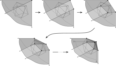
Figure 12: The new algorithm as seen from visible Euclidean space

The overall procedure is illustrated in Figure 12 (which only shows the portions of $Q_{0},Q_{1},\ldots$ in visible Euclidean 3-space, and does not show the additional points at infinity). It should be noted that all of the geometric entities used in this algorithm lie in the interior of a projective half-space, which means that all of the relevant concepts (such as polytopes, convex hulls and line segments) are properly defined.

We will shortly discuss the implementation of the various steps of this algorithm. However, our most immediate task is to prove the correctness of the algorithm as a whole.

Theorem 5.5.

Algorithm 5.4 is correct (i.e., it outputs precisely the efficient extreme outcomes for our multiobjective linear program), and it terminates in finitely many iterations.

Proof.

We prove the correctness of this algorithm in several stages.

1. For each polytope $Q_{i}$ we have $Q_{i}\supseteq T^{\leq}$:

   This is simple to prove by induction. The visible Euclidean points of the initial simplex $Q_{0}$ are precisely those with signed homogeneous coordinates of the form $(y_{1}^{\mathrm{max}}-\beta_{1},\ldots,y_{p}^{\mathrm{max}}-\beta_{p},1)$ for $\beta_{1},\ldots,\beta_{p}\geq 0$, which includes all visible Euclidean points of $T^{\leq}$. Moreover, the vertices at infinity for $Q_{0}$ are precisely the vertices at infinity for $T^{\leq}$ (Lemma 4.7). Thus $Q_{0}\supseteq T^{\leq}$.

   For the inductive step, we observe that $Q_{i+1}$ is the intersection of $Q_{i}$ with a half-space $H\supseteq T^{\leq}$ (Step 3). It follows that if $Q_{i}\supseteq T^{\leq}$ then $Q_{i+1}\supseteq T^{\leq}$ also.

2. For each polytope $Q_{i}$, the vertices at infinity are precisely the points $(-1,0,0,\ldots,0,0)$, $(0,-1,0,\ldots,0,0)$, …, $(0,0,0,\ldots,-1,0)$:

   Let $H_{\infty}$ denote the infinite hyperplane in $\mathbb{T}_{p}$ (as defined earlier in Section 3). The intersection of the initial simplex $Q_{0}$ with $H_{\infty}$ is precisely the $(p-1)$-simplex whose vertices are $(-1,0,0,\ldots,0,0)$, $(0,-1,0,\ldots,0,0)$, …, $(0,0,0,\ldots,-1,0)$. However, Definition 4.4 shows that the intersection of $T^{\leq}$ with $H_{\infty}$ is this same $(p-1)$-simplex. Because $Q_{0}\supseteq Q_{1}\supseteq\ldots\supseteq T^{\leq}$, it follows that $Q_{i}\cap H_{\infty}=T^{\leq}\cap H_{\infty}$ for each $i$, and in particular the vertices of $Q_{i}$ at infinity are the same $p$ points described above.

3. The termination condition is correct, i.e., we terminate if and only if $Q_{i}=T^{\leq}$:

   Step 1 instructs us to terminate if and only if no visible Euclidean vertex of $Q_{i}$ lies outside $T^{\leq}$. By fact (ii) above, this is equivalent to the condition that no vertex of $Q_{i}$ lies outside $T^{\leq}$. Because $Q_{i}$ and $T^{\leq}$ are both projective polytopes with $Q_{i}\supseteq T^{\leq}$, this is equivalent to the condition that $Q_{i}=T^{\leq}$.

4. The output is correct, i.e., we output precisely the set of efficient extreme outcomes for our multiobjective linear program:

   By fact (iii) above, if we terminate then we have $Q_{i}=T^{\leq}$, whereupon Step 1 instructs us to output all visible Euclidean vertices of $T^{\leq}$. Corollary 4.8 shows that these are precisely the efficient extreme outcomes for our multiobjective linear program.

Together these facts show that, if the algorithm terminates, it produces the correct results.

Our final task is to prove that the algorithm terminates in finitely many steps. Let $\partial Q_{i}$ denote the boundary of the projective polytope $Q_{i}$. Because $Q_{i}\supseteq T^{\leq}$, the intersection $\partial Q_{i}\cap T^{\leq}$ must be a union of faces of $T^{\leq}$.

We observe that each intersection $\partial Q_{i+1}\cap T^{\leq}$ is strictly larger than $\partial Q_{i}\cap T^{\leq}$, since it contains the new point $\mathbf{x}$ identified in Step 2. In particular, we know that $\mathbf{x}\notin\partial Q_{i}$, since $\mathbf{x}$ lies strictly between the vertex $\mathbf{v}$ and the interior point $\overline{\mathbf{y}}$. However, we also know that $\mathbf{x}\in\partial Q_{i+1}\cap T^{\leq}$, since Step 2 ensures that $\mathbf{x}\in T^{\leq}$ and Step 3 ensures that $\mathbf{x}\in\partial Q_{i+1}$.

It follows that each intersection $\partial Q_{i+1}\cap T^{\leq}$ contains strictly more faces of $T^{\leq}$ than the previous intersection $\partial Q_{i}\cap T^{\leq}$. Because $T^{\leq}$ has finitely many faces, this sequence cannot grow forever and the algorithm must terminate. ∎

The individual steps of Algorithm 5.4 are performed in much the same way as for the original algorithm.

• In the initialisation phase, the point $\mathbf{y}^{\mathrm{max}}$ is straightforward to compute, and for the interior point $\overline{\mathbf{y}}\in T^{\leq}$ we can simply use $\widehat{\mathbf{y}}$ from Definition 4.2. The half-space representation of the initial simplex $Q_{0}$ involves the $p$ “ordinary” half-spaces with signed homogeneous coordinates $(-1,0,0,\ldots,0,y_{1}^{\mathrm{max}})$, $(0,-1,0,\ldots,0,y_{2}^{\mathrm{max}})$, …, $(0,0,0,\ldots,-1,y_{p}^{\mathrm{max}})$, as well as the visible half-space $(0,0,0,\ldots,0,1)$.

• In Step 1 we are required to test whether a visible Euclidean vertex belongs to $T^{\leq}$. For this we can restrict our attention to visible Euclidean space (where $T^{\leq}$ becomes the Euclidean polyhedron $Y^{\leq}$), and we can employ precisely the same feasibility test used in the original algorithm.

• Likewise, Steps 2 and 3 can be performed in visible Euclidean space using the same feasibility tests, univariate search techniques and dual linear programs as before. In Step 3 it is trivial to convert the resulting half-space $H$ back into oriented projective $p$-space.

This leaves Step 4, where we must enumerate the vertices of the new polytope $Q_{i+1}$. For this we can use the double description method directly in oriented projective $p$-space:

Theorem 5.6.

The results of Theorem 5.2 and Lemma 5.3 also hold true in oriented projective $p$-space. That is, they remain true if we replace all occurrences of $\mathbb{E}_{p}$, polytopes, half-spaces and hyperplanes with $\mathbb{T}_{p}$, projective polytopes, projective half-spaces and projective hyperplanes respectively.

Proof.

Instead of offering a direct proof, we can transform these results into their Euclidean counterparts using a powerful tool known as a projective mapping. Projective mappings are geometric transformations in $\mathbb{T}_{p}$ that preserve collinearity and concurrency. They map projective hyperplanes to projective hyperplanes and projective half-spaces to projective half-spaces (and therefore projective polytopes to projective polytopes). Every projective mapping has an inverse projective mapping, and for any projective half-space $H\subseteq\mathbb{T}_{p}$ there is a projective mapping that takes $H$ to the visible half-space. For more information on projective mappings, the reader is referred to Boissonnat and Yvinec [8].

Using projective mappings, the proof of Theorem 5.6 becomes simple. If $P\subseteq\mathbb{T}_{p}$ is a projective polytope then it lies in the interior of some projective half-space $H\subseteq\mathbb{T}_{p}$. Let $\pi$ be a projective mapping that maps $H$ to the visible half-space. The interior points of $H$ map to visible Euclidean points, and $P$ therefore maps to a visible Euclidean polytope.

We can now apply Theorem 5.2 and Lemma 5.3 directly to the Euclidean polytope $\pi(P)$. Because both results are expressed purely in terms of lines, intersections, half-spaces and hyperplanes—all notions that are preserved under a projective mapping—the corresponding results are therefore true for the original projective polytope $P$. ∎

When using the double description method in this way to enumerate the vertices of $Q_{i+1}$, it is important to take into account all of the vertices of $Q_{i}$, including the vertices at infinity.

This final point highlights a key motivation for working in oriented projective geometry. In Euclidean space the double description method works only for polytopes, not unbounded polyhedra, because it requires a description of the polytope as a convex hull of its vertices. Oriented projective geometry allows us to use the double description method with unbounded Euclidean polyhedra (such as $Y^{\leq}$) by treating them as polytopes—that is, convex hulls of vertices—in $\mathbb{T}_{p}$.

5.3 Running time

The primary benefit of our new outer approximation algorithm is that we avoid constructing and analysing a large number of “unnecessary” vertices that are not efficient extreme outcomes for our multiobjective linear program. As shown in Section 4, the projective polytope $T^{\leq}$ (used in the new algorithm) has only $p$ unnecessary vertices, which are the $p$ vertices at infinity. In contrast, the Euclidean polytope $Y^{\square}$ (used in the original algorithm) has a significant number of unnecessary vertices—their number is always exponential in the number of objectives $p$ (Corollary 4.11), and can also grow at a severe rate relative to the problem size $(n,m)$ (Corollary 4.12).

Just as $Y^{\square}$ has significantly more vertices than $T^{\leq}$, we also expect the intermediate polytopes $P_{1},P_{2},\ldots$ from the original algorithm to have significantly more vertices than $Q_{1},Q_{2},\ldots$ from the new algorithm (recall that these families of polytopes successively approximate $Y^{\square}$ and $T^{\leq}$ respectively). This growth in the number of vertices has a direct impact on the running time of the outer approximation algorithm (Algorithm 5.1):

• In Step 1, the time required to search for a vertex $\mathbf{v}$ outside the target polytope $Y^{\square}$ is directly proportional to the number of vertices in the intermediate polytope $P_{i}$.

• In Step 4, the time required to run the double description method is proportional to the cube of the number of vertices: if the intermediate polytope $P_{i}$ has $V$ vertices, we have $O(V^{2})$ potential pairs $\mathbf{u}\in S_{+}$ and $\mathbf{v}\in S_{-}$ (Theorem 5.2), and for each such pair the adjacency test requires us to search through all of the vertices again (Lemma 5.3).

• More generally, the number of stages in the algorithm as a whole (that is, the number of intermediate polytopes $P_{1},\ldots,P_{k}$) depends on the number of vertices: each stage corresponds to some intermediate vertex $\mathbf{v}$ outside the target polytope $Y^{\square}$, and so with more intermediate vertices we expect more intermediate polytopes in total.

All of these observations indicate that the new algorithm should offer significant benefits over the original algorithm in terms of running time.

The only added complication for the new algorithm is that we must perform arithmetic in oriented projective $p$-space, where we work with $p+1$ coordinates at a time instead of $p$. The cost of this “extra coordinate” is negligible, and (unlike the number of vertices) does not affect the asymptotic growth of the running time at all.

6 Conclusions

In this paper we show how oriented projective geometry can be applied to the field of multiobjective linear programming, allowing us to work with efficiency-equivalent projective polytopes that are significantly less complex than their Euclidean counterparts. Polytopes (as opposed to unbounded polyhedra) are important because they support techniques such as the double description method, which operates on convex hulls of finitely many vertices. The reduction in complexity is important because it leads to a significant reduction in running time.

As a concrete illustration, we apply these techniques to the outer approximation algorithm, which is used to generate all efficient extreme outcomes for a multiobjective linear program. By working in oriented projective geometry we obtain a considerable reduction in the number of non-efficient vertices that the algorithm generates, and we show how this directly benefits the running time as a result.

We support these results with explicit asymptotic estimates on the number of non-efficient vertices generated in the old Euclidean setting and the new oriented projective setting. Using oriented projective geometry, the number of non-efficient vertices is precisely the number of objectives $p$. In the old Euclidean setting this number is at least $2^{p}-1$, and it can grow as fast as $\Omega(n^{\lfloor(p-1)/2\rfloor})$.

For applications with even a moderate number of objectives, this growth rate can be extremely high. For example, Steuer describes a blending problem with $p=8$ objectives [34]; here the number of non-efficient vertices in the old algorithm can grow like $\Omega(n^{3})$, which for large problem sizes is a significant burden. When the number of objectives is higher, as in the aircraft control design problem of Schy and Giesy with $p=70$ objectives [32], even the best-case growth rate of $2^{p}-1$ becomes crippling. In contrast, the new techniques in this paper deliver just $8$ and $70$ non-efficient vertices respectively, which is negligible in comparison.

Although we focus on the outer approximation algorithm for our application in Section 5, the underlying techniques of Sections 3 and 4 are quite general. We expect that the methods described in this paper can find many fruitful applications throughout the field of multiobjective linear programming, and that with further research the geometric and analytical insights described here can lead to new discoveries in other areas of high-dimensional optimisation.

Benjamin A. Burton
School of Mathematics and Physics, The University of Queensland
Brisbane QLD 4072, Australia
(bab@debian.org)

Melih Ozlen
School of Mathematical and Geospatial Sciences, RMIT University
GPO Box 2476V, Melbourne VIC 3001, Australia
(melih.ozlen@rmit.edu.au)

References

- [1] P. Armand and C. Malivert, Determination of the efficient set in multiobjective linear programming, J. Optim. Theory Appl. 70 (1991), no. 3, 467–489.
- [2] H. P. Benson, Further analysis of an outcome set-based algorithm for multiple-objective linear programming, J. Optim. Theory Appl. 97 (1998), no. 1, 1–10.
- [3] , Hybrid approach for solving multiple-objective linear programs in outcome space, J. Optim. Theory Appl. 98 (1998), no. 1, 17–35.
- [4] H. P. Benson and E. Sun, Outcome space partition of the weight set in multiobjective linear programming, J. Optim. Theory Appl. 105 (2000), no. 1, 17–36.
- [5] Harold P. Benson, An outer approximation algorithm for generating all efficient extreme points in the outcome set of a multiple objective linear programming problem, J. Global Optim. 13 (1998), no. 1, 1–24.
- [6] Harold P. Benson and Erjiang Sun, A weight set decomposition algorithm for finding all efficient extreme points in the outcome set of a multiple objective linear program, European J. Oper. Res. 139 (2002), no. 1, 26–41.
- [7] Albrecht Beutelspacher and Ute Rosenbaum, Projective geometry: From foundations to applications, Cambridge Univ. Press, Cambridge, 1998.
- [8] Jean-Daniel Boissonnat and Mariette Yvinec, Algorithmic geometry, Cambridge Univ. Press, Cambridge, 1998.
- [9] Pey-Chun Chen, Pierre Hansen, and Brigitte Jaumard, On-line and off-line vertex enumeration by adjacency lists, Oper. Res. Lett. 10 (1991), no. 7, 403–409.
- [10] Jared L. Cohon, Multiobjective programming and planning, Academic Press, New York, 1978.
- [11] H. S. M. Coxeter, Projective geometry, 2nd ed., Springer, New York, 1987.
- [12] J. P. Dauer and O. A. Saleh, Constructing the set of efficient objective values in multiple objective linear programs, European J. Oper. Res. 46 (1990), no. 3, 358–365.
- [13] , A representation of the set of feasible objectives in multiple objective linear programs, Linear Algebra Appl. 166 (1992), 261–275.
- [14] Jerald P. Dauer, Analysis of the objective space in multiple objective linear programming, J. Math. Anal. Appl. 126 (1987), no. 2, 579–593.
- [15] Jerald P. Dauer and Yi-Hsin Liu, Solving multiple objective linear programs in objective space, European J. Oper. Res. 46 (1990), no. 3, 350–357.
- [16] J. G. Ecker, N. S. Hegner, and I. A. Kouada, Generating all maximal efficient faces for multiple objective linear programs, J. Optim. Theory Appl. 30 (1980), no. 3, 353–381.
- [17] Gerald W. Evans, An overview of techniques for solving multiobjective mathematical programs, Management Sci. 30 (1984), no. 11, 1268–1282.
- [18] Komei Fukuda and Alain Prodon, Double description method revisited, Combinatorics and Computer Science (Brest, 1995), Lecture Notes in Comput. Sci., vol. 1120, Springer, Berlin, 1996, pp. 91–111.
- [19] Tomáš Gál, A general method for determining the set of all efficient solutions to a linear vectormaximum problem, European J. Oper. Res. 1 (1977), no. 5, 307–322.
- [20] Richard J. Gallagher and Ossama A. Saleh, A representation of an efficiency equivalent polyhedron for the objective set of a multiple objective linear program, European J. Oper. Res. 80 (1995), no. 1, 204–212.
- [21] Arthur M. Geoffrion, Proper efficiency and the theory of vector maximization, J. Math. Anal. Appl. 22 (1968), 618–630.
- [22] Branko Grünbaum, Convex polytopes, 2nd ed., Graduate Texts in Mathematics, no. 221, Springer, New York, 2003.
- [23] Reiner Horst, Jakob de Vries, and Nguyen V. Thoai, On finding new vertices and redundant constraints in cutting plane algorithms for global optimization, Oper. Res. Lett. 7 (1988), no. 2, 85–90.
- [24] H. Isermann, Proper efficiency and the linear vector maximum problem, Operations Res. 22 (1974), no. 1, 189–191.
- [25] Heinz Isermann, The enumeration of the set of all efficient solutions for a linear multiple objective program, Oper. Res. Quart. 28 (1977), no. 3, 711–725.
- [26] Kevin G. Kirby, Beyond the celestial sphere: Oriented projective geometry and computer graphics, Math. Mag. 75 (2002), no. 5, 351–366.
- [27] Stéphane Laveau and Olivier Faugeras, Oriented projective geometry for computer vision, Computer Vision—ECCV ’96, Lecture Notes in Comput. Sci., vol. 1064, Springer, Berlin, 1996, pp. 147–156.
- [28] Jiří Matoušek and Bernd Gärtner, Understanding and using linear programming, Springer, Berlin, 2007.
- [29] T. S. Motzkin, H. Raiffa, G. L. Thompson, and R. M. Thrall, The double description method, Contributions to the Theory of Games, Vol. II (H. W. Kuhn and A. W. Tucker, eds.), Annals of Mathematics Studies, no. 28, Princeton University Press, Princeton, NJ, 1953, pp. 51–73.
- [30] Anthony Przybylski, Xavier Gandibleux, and Matthias Ehrgott, A recursive algorithm for finding all nondominated extreme points in the outcome set of a multiobjective integer programme, To appear in INFORMS J. Comput., published online ahead of print, 2009.
- [31] N. Schulz, Welfare economics and the vector maximum problem, Multicriteria Optimization in Engineering and in the Sciences (Wolfram Stadler, ed.), Mathematical Concepts and Methods in Science and Engineering, vol. 37, Plenum Press, New York, 1988, pp. 77–116.
- [32] Albert A. Schy and Daniel P. Giesy, Multicriteria optimization methods for design of aircraft control systems, Multicriteria Optimization in Engineering and in the Sciences (Wolfram Stadler, ed.), Mathematical Concepts and Methods in Science and Engineering, vol. 37, Plenum Press, New York, 1988, pp. 225–262.
- [33] Wolfram Stadler (ed.), Multicriteria optimization in engineering and in the sciences, Mathematical Concepts and Methods in Science and Engineering, vol. 37, Plenum Press, New York, 1988.
- [34] Ralph E. Steuer, Sausage blending using multiple objective linear programming, Manage. Sci. 30 (1984), no. 11, 1376–1384.
- [35] , Multiple criteria optimization: Theory, computation, and application, Wiley Series in Probability and Mathematical Statistics: Applied Probability and Statistics, John Wiley & Sons Inc., New York, 1986.
- [36] Ralph E. Steuer and Craig A. Piercy, A regression study of the number of efficient extreme points in multiple objective linear programming, European J. Oper. Res. 162 (2005), no. 2, 484–496.
- [37] Jorge Stolfi, Oriented projective geometry, SCG ’87: Proceedings of the Third Annual Symposium on Computational Geometry, ACM, 1987, pp. 76–85.
- [38] , Oriented projective geometry, Academic Press, Boston, MA, 1991.
- [39] Tomáš Werner and Tomáš Pajdla, Oriented matching constraints, Proceedings of the British Machine Vision Conference 2001 (Manchester, UK) (Timothy F. Cootes and Christopher J. Taylor, eds.), British Machine Vision Association, 2001, pp. 441–450.
- [40] P. L. Yu and M. Zeleny, The set of all nondominated solutions in linear cases and a multicriteria simplex method, J. Math. Anal. Appl. 49 (1975), 430–468.
- [41] Milan Zeleny, Multiple criteria decision making, McGraw-Hill, New York, 1982.
- [42] Günter M. Ziegler, Lectures on polytopes, Graduate Texts in Mathematics, no. 152, Springer-Verlag, New York, 1995.