Surface flux transport modeling for solar cycles 15–21: effects of cycle-dependent tilt angles of sunspot groups

Abstract

We model the surface magnetic field and open flux of the Sun from 1913 to 1986 using a surface flux transport model, which includes the observed cycle-to-cycle variation of sunspot group tilts. The model reproduces the empirically derived time evolution of the solar open magnetic flux, and the reversal times of the polar fields. We find that both the polar field and the axial dipole moment resulting from this model around cycle minimum correlate with the strength of the following cycle.

1 Introduction

The evolution of the large scale magnetic field at the surface of the Sun can be modeled using a two-dimensional surface flux transport model where the magnetic fields undergo a random walk due to supergranular flows (Leighton, 1964), are advected by differential rotation and meridional circulation (Babcock, 1961; Leighton, 1964; Sheeley et al., 1983), and are subject to a slow decay from three-dimensional processes (Schrijver et al., 2002; Baumann et al., 2006). The surface field can be extrapolated out into the heliosphere, including the region near the Earth (Wang et al., 2000). This makes the historic record of the magnetic environment of the Earth, as manifested in the geomagnetic perturbation indices, a valuable constraint on the variation of the magnetic fields of the Sun. The use of the surface flux transport model as the basis for field extrapolations has received some recent attention (Mackay et al., 2002; Wang et al., 2002b; Schüssler & Baumann, 2006; Jiang et al., 2010a).

The flux transport model has been refined over time: early work assumed time-independent flows and did not include the effects of radial diffusion. It was found (Lean et al., 2002; Schrijver et al., 2002) that the observed variation in the cycle amplitudes would then lead to a secular drift of the polar field, in contradiction to observations. Two ways of extending the model were considered to cope with this problem: (1) making the meridional velocity time dependent (Wang et al., 2002a), and (2) assuming that the poloidal field decays with a timescale of about 5 years (Schrijver et al., 2002; Baumann et al., 2006). Here we consider a third possibility, namely that the tilt angle of the groups, the subject of Joy’s law, varies from cycle to cycle.

Most surface flux transport studies have used fixed differential rotation and meridional flows. Two of the exceptions are the studies of Wang et al. (2002a) and Dikpati et al. (2004) who considered cycle-to-cycle changes of the meridional flow. Wang et al. (2002a) suggested that a suitably varying time-dependent meridional flow would prevent a secular drift of the polar fields and thus allows them to reverse every cycle despite large variations in the cycle amplitudes.

Our study is motivated by the recent finding of Dasi-Espuig et al. (2010) that the tilt angles of sunspot groups from the Mount Wilson Observatory and Kodaikanal observations (Howard et al., 1984, 1999; Sivaraman et al., 1999) show a cycle-to-cycle variation of Joy’s law. Further they showed that the average tilt angle is negatively correlated with the strength of the cycle, i.e., the tilt angle is smaller for stronger cycles. A reduced tilt angle entails a smaller latitudinal separation between opposite polarity spots within a group, leading to reduced advection and diffusion of following polarity magnetic flux towards the poles during strong cycles (Cameron & Schüssler, 2007).

Here we include the observed tilt angle variations as input to the flux transport model. Doing so requires us to reconsider the various parameters which go into the model (within the range constrained by observations). In addition, we tentatively consider the effect of the observed inflows into active regions (Haber et al., 2004; Hindman et al., 2004; Komm et al., 2007) which cause a reduced escape of flux from active regions (De Rosa & Schrijver, 2006).

The paper is organized as follows: Section 2 describes the flux transport model, including a brief discussion of how well the model parameters are observationally known. Section 3 outlines the observations to which the model’s results are compared in order to further constrain the parameters and test the model. In Section 4 we give the parameters for our reference case. A brief parameter study, concentrating on the qualitative changes which occur as the different parameters are varied, is presented in Section 5. Our conclusions are given in Section 6.

2 Flux transport model

The surface flux transport model describes the passive transport of the radial component of the magnetic field, $B$, on the solar surface under the effects of differential rotation, $\Omega$, meridional flow, $v$, and surface diffusivity, $\eta_{H}$, whilst gradually decaying owing to radial diffusion (DeVore et al., 1985; Sheeley Jr et al., 1985; Wang et al., 1989; Mackay et al., 2000; Schrijver et al., 2002; Baumann et al., 2004). A source term, $S(\lambda,\phi,t)$, describes the emergence of new flux as a function of latitude, $\lambda$, and longitude, $\phi$. The governing equation is

$$\frac{\partial B}{\partial t}= -\Omega(\lambda)\frac{\partial B}{\partial\phi}-\frac{1}{R_{\bigodot}\cos\lambda}\frac{\partial}{\partial\lambda}\left[v(\lambda)B\cos\lambda\right]$$

$$+\eta_{H}\left[\frac{1}{R_{\bigodot}^{2}\cos{\lambda}}\frac{\partial}{\partial\lambda}\left(\cos\lambda\frac{\partial B}{\partial\lambda}\right)+\frac{1}{R_{\bigodot}^{2}\cos^{2}{\lambda}}\frac{\partial^{2}B}{\partial\phi^{2}}\right]$$

$$+D(\eta_{r})+S(\lambda,\phi,t),$$

where $D$ is a linear operator describing the decay due to radial diffusion with radial diffusivity $\eta_{r}$. For $D$ we adopt the form used in Baumann et al. (2006). We use the time averaged (synodic) differential rotation profile given by Snodgrass (1983): $\Omega(\lambda)=13.38-2.30\sin^{2}\lambda-1.62\sin^{4}\lambda$ (in ${}^{\circ}/$day). For the time-averaged meridional flow we use the same profile as van Ballegooijen et al. (1998), i.e.

$$v(\lambda)=\begin{cases}11\sin(2.4\lambda)\text{\,m\,s}^{-1}&\text{where}|\lambda|\leq 75^{\circ}\\ 0&\text{otherwise.}\end{cases}$$ (2)

The two remaining parameters of the flux transport model are the horizontal and radial diffusivities, $\eta_{H}$ and $\eta_{r}$. The results of various attempts to measure $\eta_{H}$ from observation are summarized in Table 6.2 of Schrijver & Zwaan (2000). The values obtained from cross-correlation and object-tracking methods fall in the range $100-300$ km²s^-1. We have used $\eta_{H}=250$ km²s^-1 for our reference value in Section 4; this value lies within the range of the observations, but we also consider the effect of varying it in Section 5.

Much less is known about $\eta_{r}$. This term was introduced by Baumann et al. (2006) to account for the 3D radial diffusion of the magnetic field and to obtain regularly reversing polar fields for cycles of varying amplitude in the absence of variations of the meridional flow. Its physical motivation is that the Sun’s magnetic field is three-dimensional and thus has more modes of decay than are captured by the two-dimensional surface diffusion. We find here that the results with $\eta_{r}=0$ match the observations well (including having the polar fields reverse each cycle) when we include the observed tilt angle variations. We thus take $\eta_{r}=0$ as our reference value and consider other values in Section 5.

For the source term $S(\lambda,\phi,t)$ in Equation 2 we follow van Ballegooijen et al. (1998) and Baumann et al. (2004) and consider new flux to emerge in the form of of opposite polarity patches. The positive-polarity patch is centered on latitude $\lambda_{+}$ and longitude $\phi_{+}$, the negative patch at $(\lambda_{-},\phi_{-})$. The field of each new bipole is given by $B=B^{+}-B^{-}$ with

$$B^{\pm}(\lambda,\phi)=B_{\mathrm{max}}\left(\frac{0.4\Delta\beta}{\delta}\right)^{2}\mathrm{exp}({2[1-\cos(\beta_{\pm}(\lambda,\phi))/\delta^{2}]}),$$ (3)

where $\beta_{\pm}(\lambda,\phi)$ are the heliocentric angles between $(\lambda,\phi)$ and $(\lambda_{\pm},\phi_{\pm})$, respectively and $\Delta\beta=\beta_{+}(\lambda_{-},\phi_{-})$ is the separation between the two polarities, and $\delta=4^{\circ}$ is the size of the individual polarity patches. For the purposes of comparing the flux transport simulations with observations it is necessary to connect $S$ closely to the actual observations. We use sunspot group areas and locations corresponding to their time of maximum area from http://solarscience.msfc.nasa.gov/greenwch.shtml (based on the Greenwich photoheliographic maps from 1874 to 1976 and USAF/NOAA SOON data thereafter) as proxies for emerging flux.

The Greenwich/USAF/NOAA record contains the locations and areas of sunspots groups, but no magnetic polarity information. We use the location and areas to construct bipolar magnetic regions with the form described by Equation 3. The location of the bipoles, $(\lambda_{\pm},\phi_{\pm})$, in the northern hemisphere are given by

$$\lambda_{\pm} = \lambda_{m}\pm(-1)^{n}0.5\Delta\beta\sin\alpha$$ (4)

$$\phi_{\pm} = \phi_{m}\mp(-1)^{n}0.5\Delta\beta\cos\alpha(\cos\lambda)^{-1},$$ (5)

and those in the southern hemisphere by

$$\lambda_{\pm} = \lambda_{m}\pm(-1)^{n}0.5\Delta\beta\sin\alpha$$ (6)

$$\phi_{\pm} = \phi_{m}\pm(-1)^{n}0.5\Delta\beta\cos\alpha(\cos\lambda)^{-1}.$$ (7)

Here $(\lambda_{m},\phi_{m})$ is the central location of the group from the Greenwich/USAF/NOAA record, $\alpha$ the tilt angle with respect to the azimuthal direction, and $n$ the cycle number. The separation, $\Delta\beta$, between the two polarities is taken to be $\Delta\beta=0.45A_{R}^{1/2}$ where $A_{R}$ is the total area of the active region. We estimate the total flux of an active region by considering its total area, $A_{R}$, to be the sum of the area covered by the sunspots $A_{s}$ and the plage $A_{p}$ using the observed relationship

$$A_{R}=A_{s}+A_{p}=A_{s}+414+21A_{s}-0.0036A_{s}^{2},$$ (8)

(Chapman et al., 1997), where all areas are measured in millionths of a solar hemisphere. The coefficient 0.45 was determined by using the sunspot group data from Mount Wilson (covering the period from 1917 to 1985) and Kodaikanal (covering the period from 1906 to 1987). The data sets are described in Howard et al. (1984) and Sivaraman et al. (1999) and are available from http://ngdc.noaa.gov/stp/SOLAR/ftpsunspotregions.html. Both data sets include umbral areas $A_{U}$ and separations $\Delta\beta$ between the “centers of mass” of the leading and following spots. We converted the umbral areas to sunspot areas using the results of Brandt et al. (1990), and from there to $A_{R}$ using Equation 8. Figure 1 shows the average (over 7-degree bins) of $\Delta\beta$ from each data set together with the fit curve.

The next step is to specify the tilt angle, $\alpha$, including its cycle-to-cycle variations. As noted in Baumann et al. (2004) the polar fields are essentially proportional to $\alpha$, so that these variations might strongly affect the results. We use the tilt angles provided by the sunspot group data from Mount Wilson and from Kodaikanal. Since these observations cover only part of the sunspot groups in the combined Greenwich/USA/NOAA dataset that we use for the source, we take cycle-averaged properties for the tilt angle as a function of latitude. The asterisks in Figure 2 show the binned cycle averages of the tilt angle weighted with the group areas. We fit the data from each cycle to the form $\alpha=T_{n}\sqrt{|\lambda|}$, where $n$ is the cycle number. We calculate $T_{n}$ by

$$T_{n}=\frac{\sum_{i}A_{i}\alpha_{i}}{\sum_{i}A_{i}\sqrt{|\lambda_{i}|}}$$ (9)

where the summation is over all spot groups in cycle $n$; $A_{i}$ is area of the $i$-th spot group and $\lambda_{i}$ is its latitude. If the tilt angle of each group of cycle $n$ is written as $\alpha_{i}=T_{n}\sqrt{|\lambda_{i}|}+\epsilon_{i}$, then the above estimate for $T_{n}$ implies $\sum_{i}A_{i}\epsilon_{i}=0$ i.e., the area-weighted sum of the deviations from the fit curve is zero. We see in Figure 2 that the square-root profile produces a reasonable fit. Furthermore cycle 19 is systematically low across a broad range of latitudes. Figure 3 shows $T_{n}$ for both the Mount Wilson and Kodaikanal data sets.

Observed localized inflows associated with active regions (Haber et al., 2004; Hindman et al., 2004; Komm et al., 2007) are important for the evolution of the surface magnetic fields (De Rosa & Schrijver, 2006) and should be included in the model. The effect of the inflows is to reduce the rate of expansion of the active region flux. This reduces the latitudinal separation of the polarities and thus the amount of net flux which can migrate to the poles. Additionally the large-scale inflows into the activity belt (Gizon & Rempel, 2008) affects the polar fields. Jiang et al. (2010b) have quantitatively studied the effects of such inflows on the polar fields, finding that a 5 m/s global inflow such as was observed during cycle 23 reduces the polar fields by 18%. The flows into individual active regions are stronger than this global-scale inflow and thus have a bigger effect (De Rosa & Schrijver, 2006). In this paper we have tentatively introduced a time-independent parameter, $g$, which we use to scale the observed tilt angles of the sunspot groups. The main effect of $g$ is to scale the amount of flux which reaches the pole against the amount of flux which emerges in the sunspot groups. We comment that the introduction of this parameter also deals with the uncertainty of how the observed group tilt angles (which are based upon the position of sunspots in continuum intensity images) are related to the tilt angles between the opposite polarity patches of the active region.

Finally we determine $B_{\mathrm{max}}$ in Equation 3 by matching the unsigned total observed flux from the Mount Wilson and Wilcox observatories with the simulation results.

For the initial magnetic field distribution at the start of the simulation we follow van Ballegooijen et al. (1998) and use an axisymmetric solution to Equation 1 with $B=\pm B_{0}$ at the poles, and which evolves almost entirely on the slow diffusive timescale:

$$B=\begin{cases}\mathrm{sign}(\lambda)B_{0}\exp{\left(\frac{-11\mathrm{ms}^{-1}\times R_{\bigodot}}{2.4\eta_{H}}\left(1+\cos 2.4\lambda\right)\right)}&\text{if }|\lambda|<75^{\circ}\\ \mathrm{sign}(\lambda)B_{0}&\text{otherwise}.\end{cases}$$ (10)

In the absence of sources, the evolution of this initial condition is dominated by the slow decay of the global field (with an e-folding time of approximately 4000 years). This choice for the functional form of the initial condition is arbitrary. The time between flux emerging and its reaching the poles is on the order of 5 years, so the polar fields for the first 5 years or so are strongly affected by the chosen form for the initial condition. We therefore exclude the first polar field maximum from our analysis of the results.

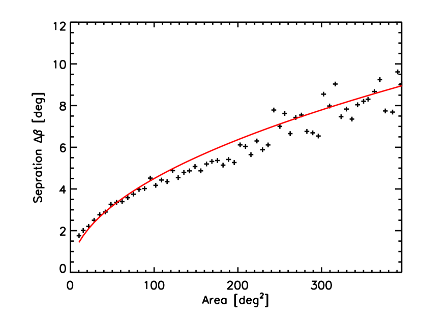
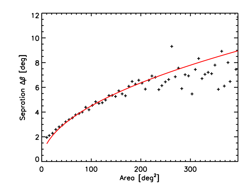
Figure 1: The separation between the following and leading polarities as a function of sunspot group area. The values are from the Kodaikanal (upper panel) and Mount Wilson Observatory data sets (lower panel). The solid red curve is the fit $\Delta\beta=0.45A_{R}^{1/2}$.

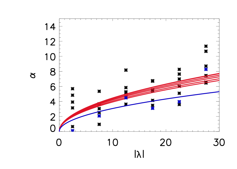
Figure 2: Area weighted tilt angle $(\sum_{i}A_{i}\alpha_{i})/(\sum_{i}A_{i})$ as a function of sunspot group latitude for cycles 15 through 21 on the basis of the combined Mt. Wilson and Kodaikanal datasets. The asterisks represent the average values for 5 degree bins for each cycle. The curves represent fits of the form $\alpha=T_{n}\sqrt{|\lambda|}$ for each cycle $n$. The blue asterisks and curve indicate cycle 19.

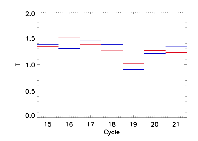
Figure 3: The cycle dependence of the factor $T_{n}$ in the fit curves of Figure 2. Shown are the values derived from the Mt. Wilson data (blue) the Kodaikanal data (red).

3 Open flux and timing of the polar reversals

The model described above requires emerging bipolar magnetic region areas, locations, and tilt angles as input. We have these data for the period between 1913 and 1986. The flux transport model gives as output the radial component of the magnetic field on the solar surface. Throughout most of the period covered by the simulations, observational magnetogram data are unavailable for comparing against the results of the simulations. We therefore consider the Sun’s open flux, ${F}_{\mathrm{open}}$, which has been inferred from the $aa$-index of geomagnetic variations (and its extensions) from 1842 onwards (Lockwood & Stamper, 1999; Lockwood, 2003). To obtain ${F}_{\mathrm{open}}$ from the simulation, we take the surface distribution of $B$ and use the current sheet source surface model (Zhao & Hoeksema, 1995a, b; Zhao et al., 2002) to extrapolate the solar surface field out into the heliosphere (see Schüssler & Baumann, 2006; Jiang et al., 2010a). The results of the extrapolation are dependent on the assumed value of the ‘cusp radius’, $R_{\mathrm{cusp}}$, which is the radial distance beyond which all the field lines are open.

We also compare the simulation results against the timing of the polar field reversals, which have been inferred by Makarov et al. (2003) from polar filament observations from 1870 to 2001.

4 Reference case

We here give the results for the parameter set $\eta_{H}=250$ km²s^-1, $g=0.7$, $B_{0}=-10.2$ G, $\eta_{r}=0$ and $R_{\mathrm{cusp}}=1.55R_{\bigodot}$. The value $B_{\mathrm{max}}=374$ G was found by matching to the total observed unsigned magnetic flux from the Mount Wilson and Wilcox Solar Observatories (see Figure 4). With these parameters, the model reproduces well the open flux ${F}_{\mathrm{open}}$  inferred by Lockwood (2003) as shown in Figure 5. This applies to the phases as well as the amplitudes of both the maxima and minima of the inferred open flux. The corresponding evolution of the polar field (defined as the average field above $\pm 75^{\circ}$ latitude) and axial dipole moment are shown in the upper panel of Figure 6. The polar field closely follows the axial dipole moment, with a delay of several years. This is understandable as the dipole moment reacts more quickly to flux transport across the equator, which then takes several additional years to reach the polar latitudes ($>75^{\circ}$). The simulated polar fields reverse for all cycles. Without the cycle-dependent variations of the tilt angle the weak cycle 20 would have been unable to offset the polar field after cycle 19. It was this type of problem which led Schrijver et al. (2002) and Baumann et al. (2006) to introduce a decay term. Here we achieve a good agreement with the observations even without such a term because of the anti-correlation in the observed tilt angles and cycle strengths (Dasi-Espuig et al., 2010). The asterisks in the upper panel of Figure 6 indicate the timings of the polar reversals as derived by Makarov et al. (2003) from H$\alpha$ polar filament data. The reversal times are reasonably well reproduced, except for the first reversal which is still affected by arbitrary form of the initial condition.

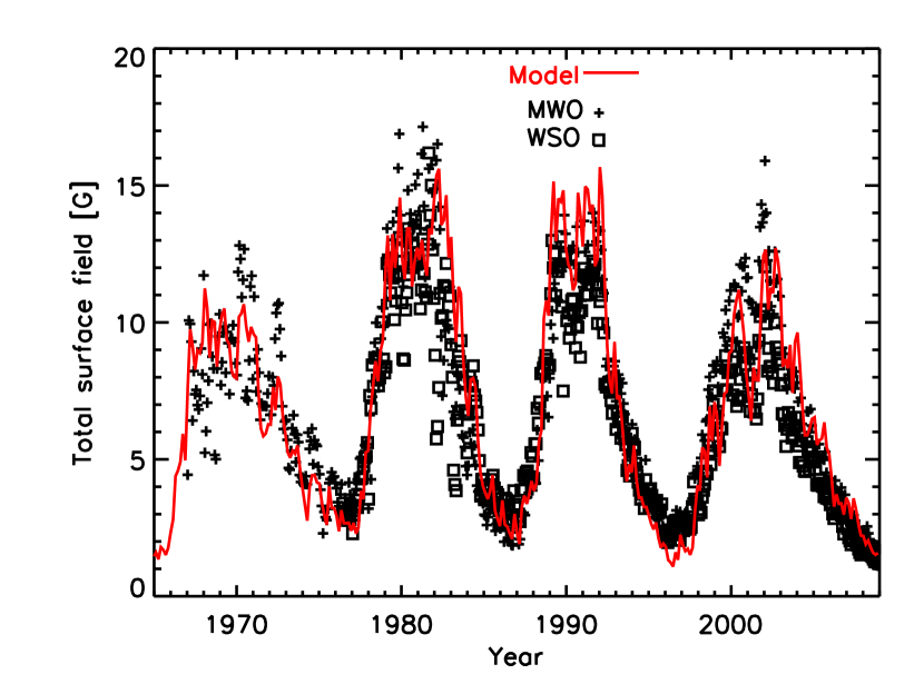
Figure 4: Average unsigned magnetic field from the simulation with $B_{\mathrm{max}}=374$ G (solid curve) compared with observations from the Mount Wilson (plus signs) and Wilcox Solar Observatories (squares).

The maximum of the dipole moment during the activity minimum between cycles 19 and 20 is much lower than that between cycles 18 and 19. This is primarily because the average tilt angle of cycle 19 was substantially lower than that of cycle 18 (see Figures 2 and 3). On the other hand, the dipole moment between cycles 20 and 21 is again high, because the average the tilt angles of cycle 20 was high. The lower panel of Figure 6 presents the time evolution of the unsigned north-south averaged polar field from the simulation as well as the observed strength of the solar activity. Ignoring the first cycle, which is strongly affected by the initial condition, the polar field can be seen to anticipate the peaks of solar activity. We have quantified this relationship by calculating the correlation between the strength of peaks the (unsigned north-south averaged) polar field and the strength of the adjacent activity maxima. As can be seen in Figure 7, the maxima of the polar field between cycles $n$ and $n+1$ reflect the amplitude of cycle $n+1$ much better than cycle $n$. The correlation coefficient for the relationship between the polar field and the amplitude of the next cycle is 0.85. This is in contrast to the result of Cameron & Schüssler (2007) who did not consider a cycle-to-cycle dependent tilt angle; they found that the polar fields and strength of the polar field closely follow the previous cycle. This indicates the importance of the cycle-to-cycle variations in the tilt angle.

Some observational evidence concerning the correlation between the polar field and the strength of the previous and subsequent cycles has been previously considered, e.g, by Schatten et al. (1978); Layden et al. (1991); Svalgaard et al. (2005); Jiang et al. (2007). The existence of a correlation between the polar field and the strength of the next cycle is evidence in favour of a Bacock-Leighton-type dynamo. Within the context of such dynamos, the correlation constrains the subsurface dynamics (see, for example, Yeates et al., 2008).

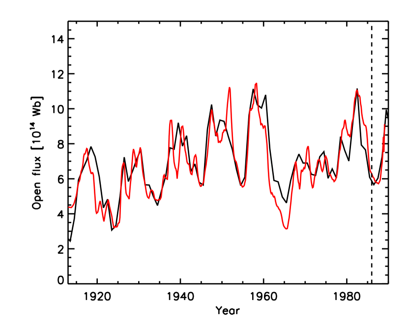
Figure 5: Open flux inferred from the $aa$-index (Lockwood, 2003, black) and result from the surface flux transport model and extrapolation (red) for the reference case. The dashed vertical black line refers to the time beyond which we have no observed values of the tilt angle.

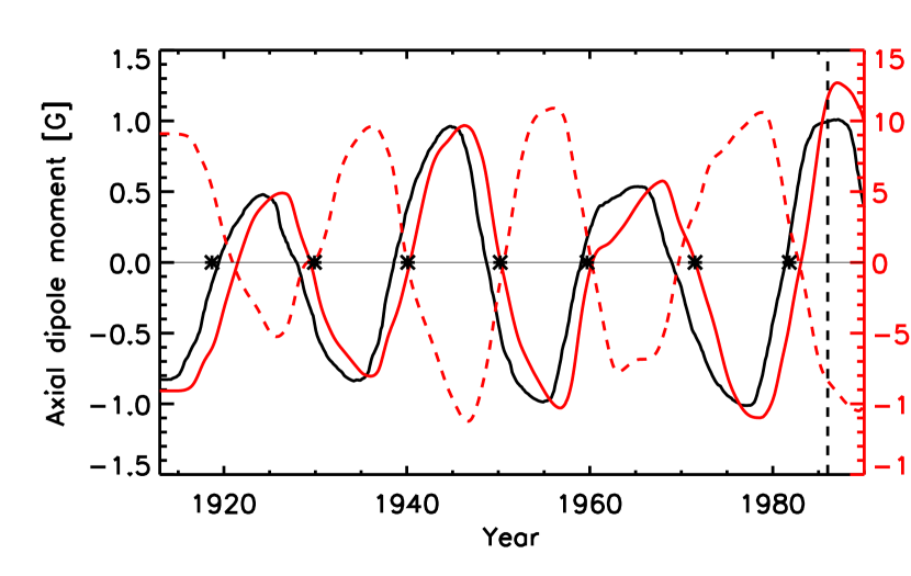
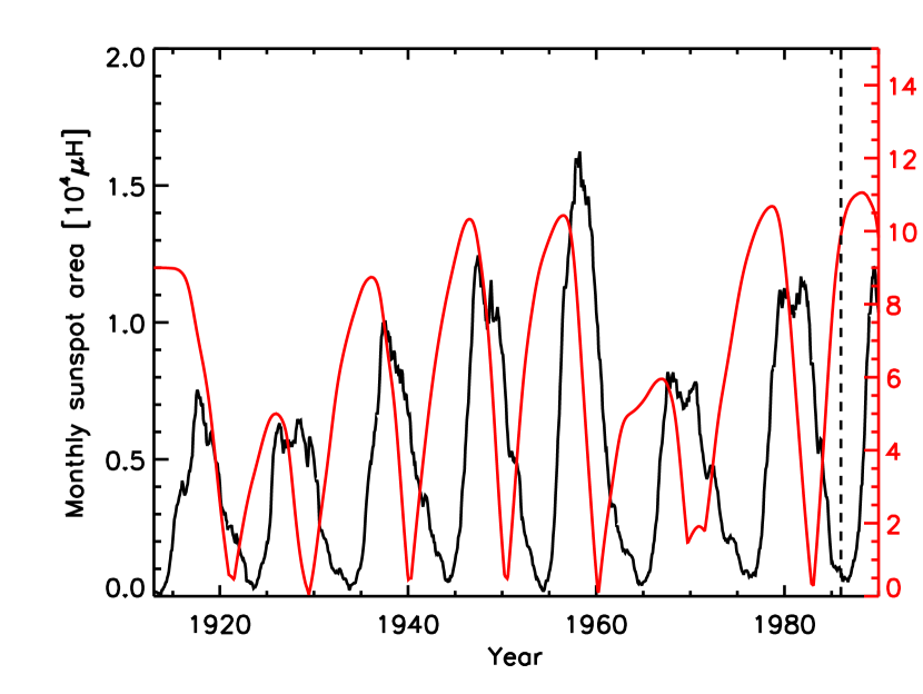
Figure 6: Upper panel: axial dipole moment (black) together with the north (solid red) and south (dashed red) polar field strengths from the flux transport simulation. The black asterisks indicate the inferred times of polar field reversals from Makarov et al. (2003). The dashed vertical black line refers to the time beyond which we have no observed values of the tilt angle. Lower panel: average of the unsigned polar field strength from the flux transport model (red) and observed sunspot area (black).

Figure 7: Correlation between the observed maximum polar field from the flux transport model and and the preceding (upper panel) and subsequent (lower panel) cycle’s maximum sunspot area. The asterisks represent the values for individual cycles: the solid line is a linear fit. The maximum sunspot area is uncorrelated ($r=-0.1$) to the subsequent polar field maximum, but strongly correlated ($r=0.85$) to the preceding polar field maximum. The first maximum of the polar field has been omitted from the analysis since it is affected by the arbitrariness of the initial field.

5 Parameter dependence

In the previous section we showed that a good representation of the empirically determined open flux ${F}_{\mathrm{open}}$  could be achieved with the parameter values of the reference model. Figure 8 shows the effect of separately varying the initial field strength, $B_{0}$, the surface diffusivity, $\eta_{H}$, radial diffusivity, $\eta_{r}$, and cusp surface height, $R_{\mathrm{cusp}}$. In all panels except the lower right we have kept $B_{\mathrm{max}}$ constant: in this panel we recalibrated $B_{\mathrm{max}}$ to account for the change in the total unsigned flux resulting from the change in $\eta_{r}$.

The upper left panel of Figure 8 shows the effect of changing $B_{0}$. Since $B_{0}$ describes the initial polar field, varying this value leads to an offset in the strength of the axial dipole moment, which persists throughout the simulation when $\eta_{r}=0$. This offset results in alternating cycles having either stronger or weaker axial dipole moments depending on whether or not they have the same sign of dipole moment as that of the initial state. Near activity minima it is the lower order axial moments which dominate ${F}_{\mathrm{open}}$  so that the minima alternately become higher and lower.

The upper right panel of Figure 8 shows the effect of increasing $\eta_{H}$: the minima of ${F}_{\mathrm{open}}$  are shifted upwards, while the maxima are not substantially affected. The explanation for the upward shift is that $\eta_{H}$ determines the amount of flux which crosses the equator and thus directly influences the axial dipole moment. There is also a weak but noticeable 22-year component, with the minima of alternating cycles being weaker. This 22-year component is present because we have not recalibrated $B_{0}$.

The middle left panel of Figure 8 shows the effect of increasing $\eta_{r}$. The enhanced decay of the field not only reduces ${F}_{\mathrm{open}}$  around the minima but also during the rise phase a cycle. This leads to too low minima and a delay of the rising phase. There is again a 22-year component because $B_{0}$ has not been recalibrated.

The middle right panel shows the effect of varying the tilt angle reduction factor, $g$, from $0.7$ to 1, which modifies the magnitude of the polar fields and axial dipole moment. The signature is therefore an increase in the magnitude of the changes in the dipole moment (and thus ${F}_{\mathrm{open}}$) its minima, so that the effect almost cancels after two cycles. This also produces a strong 22 year periodicity in the minima. We comment that $g=0.7$ is required to obtain the correct ratio between the maxima and minima of the open flux, as it essentially scales the low-order axial multipoles whilst barely affecting the equatorial multipoles. Introducing $g$ does not affect whether or not the polar fields reverse – the 22 year periodicity, when $g$ is varied in isolation, can be removed by an appropriate choice of $B_{0}$.

The lower left panel shows that increasing $R_{\mathrm{cusp}}$ in isolation weakens ${F}_{\mathrm{open}}$. The effect is strongest during the maxima as it preferentially reduces the contribution from higher order multipoles. The influence is thus qualitatively different from that of the other parameters in that it changes the relative contributions of the different multipoles.

In the panels discussed so far we have kept $B_{\mathrm{max}}$, the scaling factor for the total flux of newly emerging BMRs, constant. Varying $\eta_{r}$ as was done in the middle left panel changes the total amount of unsigned flux, and so affects the calibration of $B_{\mathrm{max}}$. In the bottom right panel we therefore show the effect of a change in $\eta_{r}$ together with the corresponding change in $B_{\mathrm{max}}$. Since the entire system is linear in $B_{\mathrm{max}}$, changing $B_{\mathrm{max}}$ merely rescales the result – hence the result in the lower right panel is just a scaled version of the result shown middle left panel. We note that varying $\eta_{H}$ also affects the calibration.

This brief study of the effect of varying the parameters illustrates the kind of changes which occur. However, it does not rule out other choices for the parameters which also could provide a good fit to the observations. In particular we do not claim that non-zero values of $\eta_{r}$ are excluded, although we can say that, at least for cycles 15–21, a good fit to the observations does not require a non-zero $\eta_{r}$.

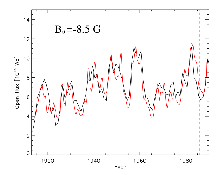
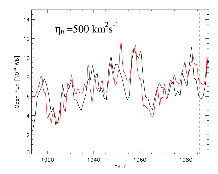
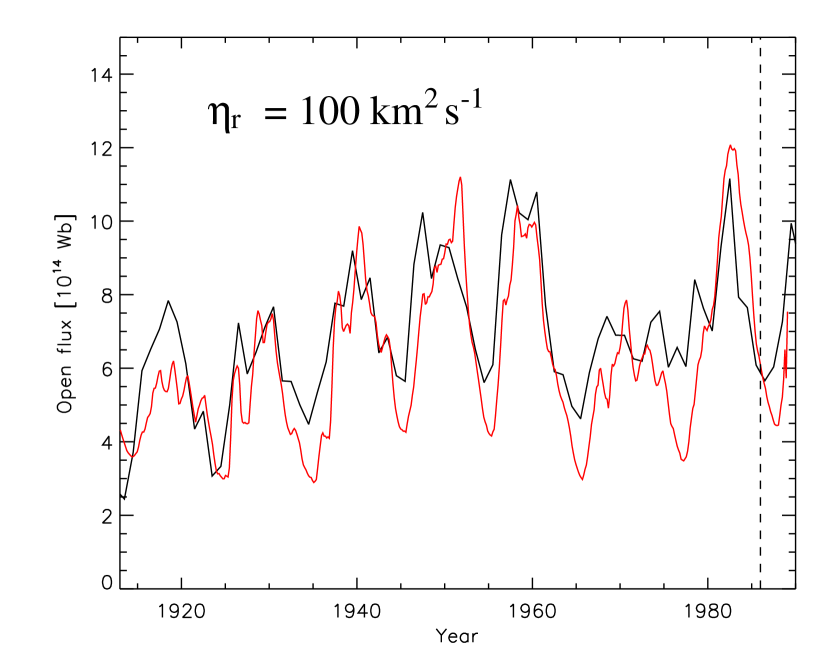
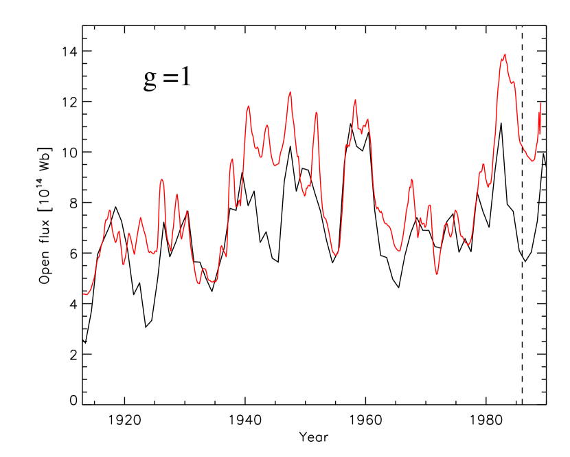
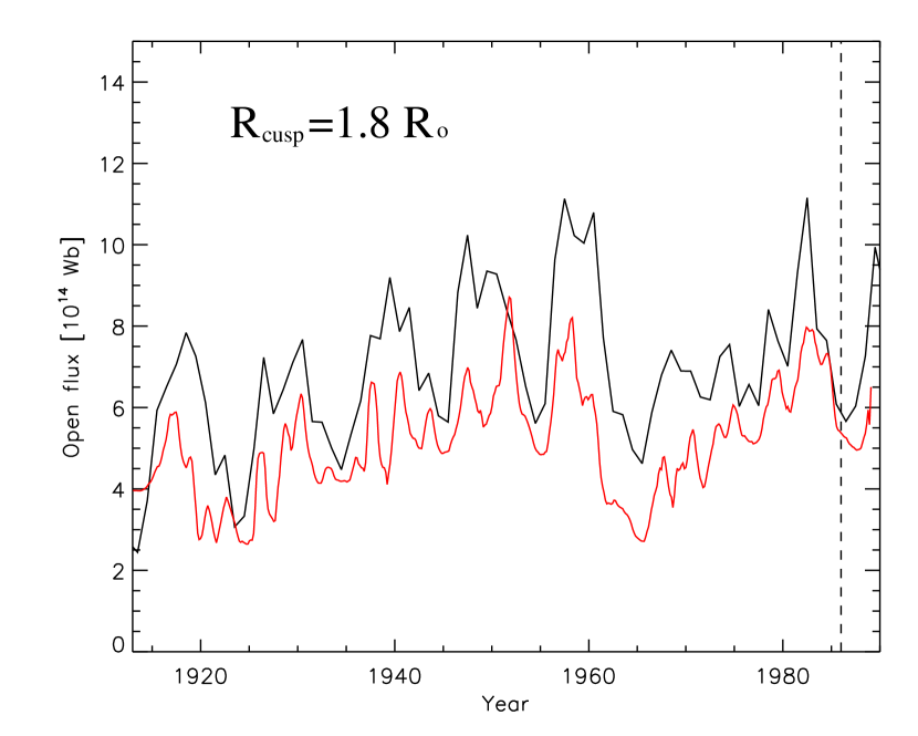
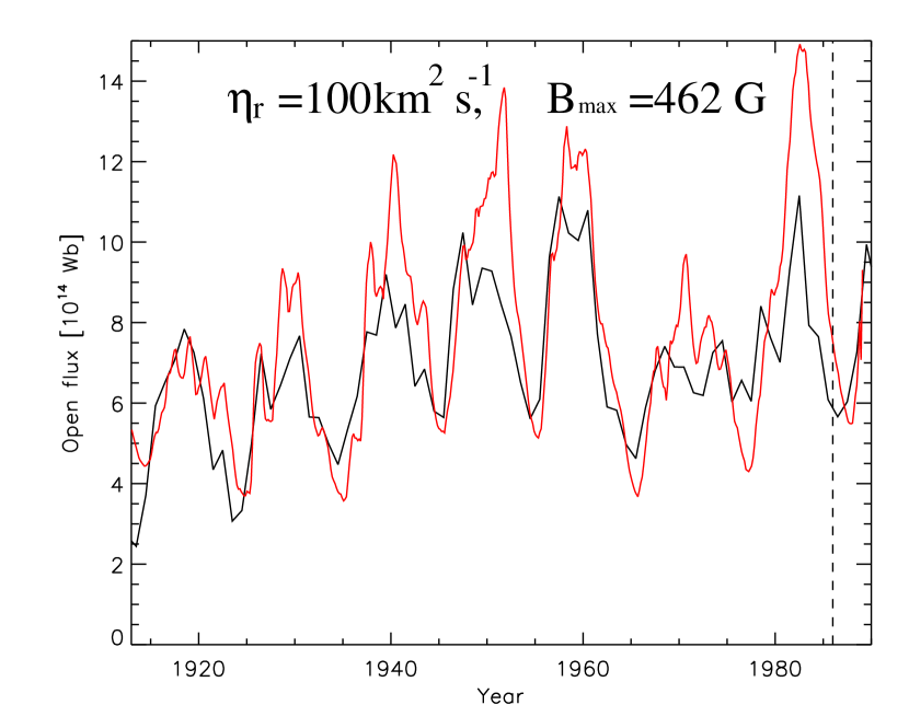
Figure 8: Effect on ${F}_{\mathrm{open}}$  of varying the parameters of the flux transport model. The black curve in each case is the observationally inferred open flux while the red curve shows the value from the simulation. For all other parameters the reference values were used. The parameters varied were:
          upper left: initial field strength $B_{0}$ ($-10.2$ G $\rightarrow$ $-8.5$ G),
                  right: surface diffusivity $\eta_{H}$ (250 km²s^-1 $\rightarrow$ $500$ km²s^-1),
          middle left: radial diffusivity $\eta_{r}$ (0 $\rightarrow 100$ km²s^-1 ),
                  right: tilt angle reduction due to inflows $g$ (0.7$\rightarrow$1)
          lower left: cusp surface radius $R_{\mathrm{cusp}}$ ($1.55R_{\bigodot}\rightarrow 1.8R_{\bigodot}$)
                  right: radial diffusivity $\eta_{r}$ ($0\rightarrow 100$ km²s^-1) and $B_{\mathrm{max}}$($374$ G $\rightarrow 462$ G)

6 Conclusions

The surface flux transport model including the effect of a cycle-dependent variation of the tilt angles of sunspot groups reproduces the major features of the observationally inferred open flux and the timing of the polar field reversals from 1913 to 1986 (the period for which we have the tilt angle data). The reversal of polar fields after strong cycles can be explained by the observed anti-correlation between the active region tilt angle and cycle amplitude, so that no additional decay by radial diffusion was required to achieve this result.

When the observed tilt angle are used, the polar field maxima from the model are correlated with the strength of the following cycle. This correlation is likely to be present independent of the parameter choices, provided the model reproduces the minima of the inferred open flux. The correlation suggests that the polar fields are an important ingredient of the solar dynamo process, which is consistent with Babcock-Leighton-type models. The cycle-to-cycle variation of Joy’s law might play a role in the nonlinear modulation of the solar dynamo.

References

- Babcock (1961) Babcock, H. W. 1961, ApJ, 133, 572
- Baumann et al. (2006) Baumann, I., Schmitt, D., & Schüssler, M. 2006, A&A, 446, 307
- Baumann et al. (2004) Baumann, I., Schmitt, D., Schüssler, M., & Solanki, S. K. 2004, A&A, 426, 1075
- Brandt et al. (1990) Brandt, P. N., Schmidt, W., & Steinegger, M. 1990, Sol. Phys., 129, 191
- Cameron & Schüssler (2007) Cameron, R. & Schüssler, M. 2007, ApJ, 659, 801
- Chapman et al. (1997) Chapman, G. A., Cookson, A. M., & Dobias, J. J. 1997, ApJ, 482, 541
- Dasi-Espuig et al. (2010) Dasi-Espuig, M., Solanki, S. K., Krivova, N. A., Cameron, R. H., & Peñuela, T. 2010, ArXiv e-prints
- De Rosa & Schrijver (2006) De Rosa, M. L. & Schrijver, C. J. 2006, in ESA Special Publication, Vol. 624, Proceedings of SOHO 18/GONG 2006/HELAS I, Beyond the spherical Sun, 12
- DeVore et al. (1985) DeVore, C., Boris, J., Young Jr, T., Sheeley Jr, N., & Harvey, K. 1985, Aust. J. Phys., 38, 999
- Dikpati et al. (2004) Dikpati, M., de Toma, G., Gilman, P. A., Arge, C. N., & White, O. R. 2004, ApJ, 601, 1136
- Gizon & Rempel (2008) Gizon, L. & Rempel, M. 2008, Sol. Phys., 251, 241
- Haber et al. (2004) Haber, D. A., Hindman, B. W., Toomre, J., & Thompson, M. J. 2004, Sol. Phys., 220, 371
- Hindman et al. (2004) Hindman, B. W., Gizon, L., Duvall, Jr., T. L., Haber, D. A., & Toomre, J. 2004, ApJ, 613, 1253
- Howard et al. (1984) Howard, R., Gilman, P. I., & Gilman, P. A. 1984, ApJ, 283, 373
- Howard et al. (1999) Howard, R. F., Gupta, S. S., & Sivaraman, K. R. 1999, Sol. Phys., 186, 25
- Jiang et al. (2010a) Jiang, J., Cameron, R., Schmitt, D., & Schüssler, M. 2010a, ApJ, 709, 301
- Jiang et al. (2007) Jiang, J., Chatterjee, P., & Choudhuri, A. R. 2007, MNRAS, 381, 1527
- Jiang et al. (2010b) Jiang, J., Işıik, E., Cameron, R., Schmitt, D., & Schüssler, M. 2010b, ApJ, in press
- Komm et al. (2007) Komm, R., Howe, R., Hill, F., Miesch, M., Haber, D., & Hindman, B. 2007, ApJ, 667, 571
- Layden et al. (1991) Layden, A. C., Fox, P. A., Howard, J. M., Sarajedini, A., & Schatten, K. H. 1991, Sol. Phys., 132, 1
- Lean et al. (2002) Lean, J. L., Wang, Y., & Sheeley, N. R. 2002, Geophys. Res. Lett., 29, 240000
- Leighton (1964) Leighton, R. B. 1964, ApJ, 140, 1547
- Lockwood (2003) Lockwood, M. 2003, J. Geophys. Res., 108, 1128
- Lockwood & Stamper (1999) Lockwood, M. & Stamper, R. 1999, Geophys. Res. Lett., 26, 2461
- Mackay et al. (2000) Mackay, D., Gaizauskas, V., & van Ballegooijen, A. 2000, ApJ., 544, 1122
- Mackay et al. (2002) Mackay, D. H., Priest, E. R., & Lockwood, M. 2002, Sol. Phys., 209, 287
- Makarov et al. (2003) Makarov, V. I., Tlatov, A. G., & Sivaraman, K. R. 2003, Sol. Phys., 214, 41
- Schatten et al. (1978) Schatten, K., Scherrer, P., Svalgaard, L., & Wilcox, J. 1978, Geophys. Res. Lett., 5, 411
- Schrijver et al. (2002) Schrijver, C. J., De Rosa, M. L., & Title, A. M. 2002, ApJ, 577, 1006
- Schrijver & Zwaan (2000) Schrijver, C. J. & Zwaan, C. 2000, Solar and stellar magnetic activity. (Cambridge University Press)
- Schüssler & Baumann (2006) Schüssler, M. & Baumann, I. 2006, A&A, 459, 945
- Sheeley et al. (1983) Sheeley, Jr., N. R., Boris, J. P., Young, Jr., T. R., Devore, C. R., & Harvey, K. L. 1983, in IAU Symposium, Vol. 102, Solar and Stellar Magnetic Fields: Origins and Coronal Effects, ed. J. O. Stenflo, 273
- Sheeley Jr et al. (1985) Sheeley Jr, N., DeVore, C., & Boris, J. 1985, Sol. Phys., 98, 219
- Sivaraman et al. (1999) Sivaraman, K. R., Gupta, S. S., & Howard, R. F. 1999, Sol. Phys., 189, 69
- Snodgrass (1983) Snodgrass, H. B. 1983, ApJ, 270, 288
- Svalgaard et al. (2005) Svalgaard, L., Cliver, E., & Kamide, Y. 2005, Geophys. Res. Lett., 32, L01104
- van Ballegooijen et al. (1998) van Ballegooijen, A. A., Cartledge, N. P., & Priest, E. R. 1998, ApJ, 501, 866
- Wang et al. (2000) Wang, Y., Lean, J., & Sheeley, N. R. 2000, Geophys. Res. Lett., 27, 505
- Wang et al. (2002a) Wang, Y., Lean, J., & Sheeley, Jr., N. R. 2002a, ApJ, 577, L53
- Wang et al. (2002b) Wang, Y., Sheeley, Jr., N. R., & Lean, J. 2002b, ApJ, 580, 1188
- Wang et al. (1989) Wang, Y.-M., Nash, A., & Sheeley Jr, N. 1989, Science, 245, 712
- Yeates et al. (2008) Yeates, A. R., Nandy, D., & Mackay, D. H. 2008, ApJ, 673, 544
- Zhao & Hoeksema (1995a) Zhao, X. & Hoeksema, J. T. 1995a, Space Sci. Rev., 72, 189
- Zhao & Hoeksema (1995b) —. 1995b, J. Geophys. Res., 100, 19
- Zhao et al. (2002) Zhao, X. P., Hoeksema, J. T., & Rich, N. B. 2002, Adv. Space Res., 29, 411