Kadanoff-Baym approach to time-dependent quantum transport in AC and DC fields

Abstract

We have developed a method based on the embedded Kadanoff-Baym equations to study the time evolution of open and inhomogeneous systems. The equation of motion for the Green’s function on the Keldysh contour is solved using different conserving many-body approximations for the self-energy. Our formulation incorporates basic conservation laws, such as particle conservation, and includes both initial correlations and initial embedding effects, without restrictions on the time-dependence of the external driving field. We present results for the time-dependent density, current and dipole moment for a correlated tight binding chain connected to one-dimensional non-interacting leads exposed to DC and AC biases of various forms. We find that the self-consistent 2B and GW approximations are in extremely good agreement with each other at all times, for the long-range interactions that we consider. In the DC case we show that the oscillations in the transients can be understood from interchain and lead-chain transitions in the system and find that the dominant frequency corresponds to the HOMO-LUMO transition of the central wire. For AC biases with odd inversion symmetry odd harmonics to high harmonic order in the driving frequency are observed in the dipole moment, whereas for asymmetric applied bias also even harmonics have considerable intensity. In both cases we find that the HOMO-LUMO transition strongly mixes with the harmonics leading to harmonic peaks with enhanced intensity at the HOMO-LUMO transition energy.

1 Introduction

The progress in miniaturization of electronic devices has led to a completely new field of research, known as molecular electronics, in which it has become possible to prepare samples and to measure steady state conductivity properties of systems with single molecules squeezed between conducting electrodes [1, 2]. However, in future applications of nanodevices one is not only interested in their steady properties, but one also wants to manipulate these systems in time. For the control and operation of such devices the understanding of the time-dependent properties, such as switch-on times, currents, density fluctuations etc., becomes crucially important. In contrast to the steady-state approach, understanding these phenomena demands truly real-time treatment of the problem which is the topic of this paper.
The study of periodic pulses is of special importance to manipulate and control the electron flow in nanoscale devices. In this paper we present results obtained from the solution of the Kadanoff-Baym (KB) equations for periodic voltage pulses. Within this framework also periodic gate voltages or barriers can be included without any additional computational effort. All these kind of signals can be experimentally realized and have been used to pump the electron current in several nanoscale structures ranging from molecules and quantum dots [3, 4] to nanotubes [5, 6]. The AC transport properties of nanoscale systems have been discussed recently [7, 8, 9, 10] and moreover, the advantages of real-time approaches in the context of quantum transport through molecular junctions driven out of equilibrium by periodic fields have been discussed in detail in Ref. [11].

There is another reason for studying AC fields in quantum transport. Usually the assumption is made that the external field in the leads is instantaneously screened. However, in time-dependent transport transient times can be of the same order as the plasma oscillation period (see e.g. Ref.[8]). In such a case it would be reasonable to assume that at Hartree mean-field level the bias in the leads can be described by an AC field that alternates with the plasma frequency.

In this article we use a recently proposed theoretical framework [12, 13] to study time-dependent electron transport through a quantum wire connected to two one-dimensional metallic leads in the presence AC and DC fields. The theoretical approach is based on the real-time propagation of the KB equations [14, 15, 16, 17, 18, 19, 20] for open and interacting systems. The electron-electron interactions are handled perturbatively through the many-body self-energy for which we have implemented the HF (Hartree Fock), 2B (Second Born) and GW conserving approximations while the leads are taken into account through embedding self-energies. We can calculate a wealth of observables such as currents, densities and dipole moments, and study electronic and initial correlations induced by the time nonlocal self-energy.

2 Theory

Figure 1: A) The transport setup under consideration: A correlated central region is coupled to semi-infinite left and right noninteracting tight-binding leads. B) The Keldysh contour $\gamma$. Times on the upper/lower real-time branches are denoted with $t_{\mp}$. The imaginary (thermal) track runs from $t_{0}$ to $t_{0}-i\beta$, with $\beta$ the inverse temperature.

2.1 The Hamiltonian

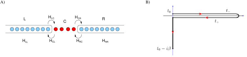
We consider a quantum correlated open system (a central region) coupled to noninteracting electron reservoirs (leads) and described by the Hamiltonian (see Fig.1 A)

$$\hat{H}(t)=\hat{H}_{\rm C}(t)+\sum_{\alpha=L,R}\hat{H}_{\alpha}(t)+\hat{H}_{T}-\mu\hat{N}.$$ (1)

Here $\hat{H}_{\rm C}$, $\hat{H}_{\alpha}$ and $\hat{H}_{T}$ are the central region, the lead $\alpha=L,R$ and the tunneling Hamiltonians respectively, and $\hat{N}$ is the particle number operator coupled to the chemical potential $\mu$. The explicit expressions for these Hamiltonians read

$$\hat{H}_{\rm C}(t) = \sum_{ij,\sigma}h_{ij}(t)\hat{d}_{i\sigma}^{\dagger}\hat{d}_{j\sigma}+\frac{1}{2}\sum_{\begin{subarray}{c}ijkl\\ \sigma\sigma^{\prime}\end{subarray}}v_{ijkl}\hat{d}_{i\sigma}^{\dagger}\hat{d}_{j\sigma^{\prime}}^{\dagger}\hat{d}_{k\sigma^{\prime}}\hat{d}_{l\sigma},$$ (2)

$$\hat{H}_{\alpha}(t) = U_{\alpha}(t)\hat{N}_{\alpha}+\sum_{ij,\sigma}h_{ij}^{\alpha}\,\hat{c}_{i\sigma\alpha}^{\dagger}\hat{c}_{j\sigma\alpha},$$ (3)

$$\hat{H}_{T} = \sum_{ij,\sigma\alpha}V_{i,j\alpha}[\hat{d}_{i\sigma}^{\dagger}\hat{c}_{j\sigma\alpha}+\hat{c}_{j\sigma\alpha}^{\dagger}\hat{d}_{i\sigma}],$$ (4)

where $\sigma,\sigma^{\prime}$ are the spin indices, $\hat{d}^{\dagger},\hat{d}$ and $\hat{c}^{\dagger}$,$\hat{c}$ are the creation and annihilation operators in the device and lead region and $i,j$ label a complete set of one-particle states in the corresponding subspaces of the system. The one-body part $h_{ij}(t)$ of the central region Hamiltonian is in general time-dependent to account for driving fields such as gate voltages or pumping fields. The terms $v_{ijkl}$ in the two-body part are the two-electron integrals of the Coulomb interaction. Furthermore, the one-body part $h_{ij}^{\alpha}$ of the lead Hamiltonian describes the metallic leads and the tunneling Hamiltonian $\hat{H}_{T}$ contains the lead couplings to the central region. The system is driven out of equilibrium by a homogeneous time-dependent bias voltage $U_{\alpha}(t)$ coupled to the number operator $\hat{N}_{\alpha}=\sum_{i,\sigma}\hat{c}_{i\sigma\alpha}^{\dagger}\hat{c}_{i\sigma\alpha}$ for lead $\alpha$. This field can be considered as the sum of the externally applied field and the resulting screening field of the metallic leads which could, for instance, represent an AC field describing a plasmon oscillation.

2.2 Kadanoff-Baym equations for the Keldysh Green’s function

We study a system that is in equilibrium at an inverse temperature $\beta$ at times $t\leq t_{0}$ and described by a Hamiltonian $\hat{H}_{0}$. For $t>t_{0}$ the system is driven out of equilibrium by an external bias voltage and evolves in time according to the Hamiltonian $\hat{H}(t)$. The Keldysh Green’s function for this system is defined as the expectation value of the contour-ordered product of the creation and annihilation operators [15, 19, 21, 22]

$$\mbox{\boldmath$\mathcal{G}$}_{rs}(z,z^{\prime})=-i\frac{{\rm Tr}\left\{\mathcal{T}[e^{-i\int d\bar{z}\hat{H}(\bar{z})}\hat{a}_{r}(z)\hat{a}^{\dagger}_{s}(z^{\prime})]\right\}}{{\rm Tr}\left\{e^{-\beta\hat{H}_{0}}\right\}},$$ (5)

where $\hat{a}$ and $\hat{a}^{\dagger}$ are either lead or central region operators and the indices $r$ and $s$ are collective indices for position and spin. Furthermore, $z$ is a contour time variable and $\mathcal{T}$ orders the operators along the Keldysh contour (see Fig.1 B) by arranging the operators with later contour times to the left. The trace is taken over the many-body states of the system. All the time-dependent one-particle properties can be calculated from the Green’s function, for example the time-dependent density matrix is given by

$$n_{rs}(t)=-i\mbox{\boldmath$\mathcal{G}$}_{rs}(t_{-},t_{+}),$$ (6)

where the time arguments $t_{\pm}$ are located on the lower/upper branch of the Keldysh contour. Starting from Eq. (5) the equation of motion for the Green’s function and its adjoint can easily be derived and are given by

$$i\partial_{z}\mbox{\boldmath$\mathcal{G}$}(z,z^{\prime}) = \delta(z,z^{\prime})\mathbf{1}+\mathbf{H}(z)\mbox{\boldmath$\mathcal{G}$}(z,z^{\prime})+\int_{\gamma}d\bar{z}\,\mbox{\boldmath$\Sigma$}^{\rm MB}(z,\bar{z})\mbox{\boldmath$\mathcal{G}$}(\bar{z},z^{\prime}),$$ (7)

$$-i\partial_{z^{\prime}}\mbox{\boldmath$\mathcal{G}$}(z,z^{\prime}) = \delta(z,z^{\prime})\mathbf{1}+\mbox{\boldmath$\mathcal{G}$}(z,z^{\prime})\mathbf{H}(z^{\prime})+\int_{\gamma}d\bar{z}\,\mbox{\boldmath$\mathcal{G}$}(z,\bar{z})\mbox{\boldmath$\Sigma$}^{\rm MB}(\bar{z},z^{\prime}),$$ (8)

where $\mbox{\boldmath$\Sigma$}^{\rm MB}$ is the many-body self-energy, $\mathbf{H}(z)$ is the one-body part of the full Hamiltonian and the integration is performed over the Keldysh-contour. These equations of motion need to be solved with the Kubo-Martin-Schwinger (KMS) boundary conditions: $\mbox{\boldmath$\mathcal{G}$}(t_{0},z^{\prime})=-\mbox{\boldmath$\mathcal{G}$}(t_{0}-i\beta,z^{\prime})$ and $\mbox{\boldmath$\mathcal{G}$}(z,t_{0})=-\mbox{\boldmath$\mathcal{G}$}(z,t_{0}-i\beta)$. All the quantities are considered as block matrices with a structure given by

$$\mathbf{H}=\left[\begin{array}[]{ccc}\mathbf{H}_{\textnormal{\scriptsize{LL}}}&\mathbf{H}_{\textnormal{\scriptsize{LC}}}&\mathbf{0}\\ \mathbf{H}_{\textnormal{\scriptsize{CL}}}&\mathbf{H}_{\textnormal{\scriptsize{CC}}}&\mathbf{H}_{\textnormal{\scriptsize{CR}}}\\ \mathbf{0}&\mathbf{H}_{\textnormal{\scriptsize{RC}}}&\mathbf{H}_{\textnormal{\scriptsize{RR}}}\end{array}\right]\,\,,\,\,\mbox{\boldmath$\Sigma$}^{\rm{MB}}=\left[\begin{array}[]{ccc}\mathbf{0}&\mathbf{0}&\mathbf{0}\\ \mathbf{0}&\mbox{\boldmath$\Sigma$}^{\rm{MB}}_{\rm{CC}}[\mbox{\boldmath$\mathcal{G}$}_{\rm{CC}}]&\mathbf{0}\\ \mathbf{0}&\mathbf{0}&\mathbf{0}\end{array}\right]\,\,,\,\,\mbox{\boldmath$\mathcal{G}$}=\left[\begin{array}[]{ccc}\mbox{\boldmath$\mathcal{G}$}_{\textnormal{\scriptsize{LL}}}&\mbox{\boldmath$\mathcal{G}$}_{\textnormal{\scriptsize{LC}}}&\mbox{\boldmath$\mathcal{G}$}_{\textnormal{\scriptsize{LR}}}\\ \mbox{\boldmath$\mathcal{G}$}_{\textnormal{\scriptsize{CL}}}&\mbox{\boldmath$\mathcal{G}$}_{\textnormal{\scriptsize{CC}}}&\mbox{\boldmath$\mathcal{G}$}_{\textnormal{\scriptsize{CR}}}\\ \mbox{\boldmath$\mathcal{G}$}_{\textnormal{\scriptsize{RL}}}&\mbox{\boldmath$\mathcal{G}$}_{\textnormal{\scriptsize{RC}}}&\mbox{\boldmath$\mathcal{G}$}_{\textnormal{\scriptsize{RR}}}\end{array}\right],$$ (9)

where the different block matrices describe the projections onto different subregions. We assume that there is no direct coupling between the leads. The many-body self-energy has nonzero elements only in the central region. This follows immediately from the diagrammatic expansion of the self-energy. More specifically, if we expand the self-energy in powers of the two-body interactions we see that the interaction matrix elements $v_{ijkl}$ only connect sites in the central region and therefore all Green function lines in the corresponding Feynman diagrams are of the type $\mbox{\boldmath$\mathcal{G}$}_{\rm{CC}}$. Therefore $\mbox{\boldmath$\Sigma$}^{\rm{MB}}[\mbox{\boldmath$\mathcal{G}$}_{\rm{CC}}]$ is a functional of $\mbox{\boldmath$\mathcal{G}$}_{\rm{CC}}$ only. Note that we do not expand in the lead-device couplings which are all exactly incorporated in the one-body matrix $\mathbf{H}$. To study the dynamical processes and to extract the observables of interest such as the densities and currents in the whole open and connected system we need the solution for the full Green function in different subregions of the system. In particular we need the Green’s functions $\mbox{\boldmath$\mathcal{G}$}_{\rm{CC}}$ projected onto central region C and $\mbox{\boldmath$\mathcal{G}$}_{\alpha\alpha}$ projected onto the lead $\alpha$ region. For these we need to extract from the block matrix structure of the Green’s function an equation for $\mbox{\boldmath$\mathcal{G}$}_{\rm{CC}}$ and $\mbox{\boldmath$\mathcal{G}$}_{\alpha\alpha}$. The projection of the equation of motion (7) onto regions ${\rm CC}$ and $\alpha{\rm C}$ gives

$$\begin{split}&\Bigl{\{}i\partial_{z}\mathbf{1}-\mathbf{H}_{\rm CC}(z)\Bigr{\}}\mbox{\boldmath$\mathcal{G}$}_{\rm CC}(z,z^{\prime})=\delta(z,z^{\prime})\mathbf{1}\,\,+\sum_{\alpha}\mathbf{H}_{{\rm C}\alpha}\mbox{\boldmath$\mathcal{G}$}_{\alpha\rm C}(z,z^{\prime})+\int_{\gamma}d\bar{z}\,\mbox{\boldmath$\Sigma$}_{\rm CC}^{\rm MB}(z,\bar{z})\mbox{\boldmath$\mathcal{G}$}_{\rm CC}(\bar{z},z^{\prime}),\end{split}$$ (10)

for the central region and

$$\Bigl{\{}i\partial_{z}\mathbf{1}-\mathbf{H}_{\alpha\alpha}(z)\Bigr{\}}\mbox{\boldmath$\mathcal{G}$}_{\alpha\rm{C}}(z,z^{\prime})=\mathbf{H}_{\alpha\rm{C}}\mbox{\boldmath$\mathcal{G}$}_{\rm{CC}}(z,z^{\prime}),$$ (11)

for the projection on the interface $\alpha{\rm C}$ region. We see that the right hand side of Eq.(11) is of a simple form as a result of the absence of two-body interactions in the leads. The uncontacted and biased lead Green’s function $\mbox{\boldmath$g$}_{\alpha\alpha}$ satisfies the equation of motion

$$\Bigl{\{}i\partial_{z}\mathbf{1}-\mathbf{H}_{\alpha\alpha}(z)\Bigr{\}}\mbox{\boldmath$g$}_{\alpha\alpha}(z,z^{\prime})=\delta(z,z^{\prime})\mathbf{1}.$$ (12)

Using this equation we can construct the solution for $\mbox{\boldmath$\mathcal{G}$}_{\alpha\rm{C}}$ and it reads

$$\mbox{\boldmath$\mathcal{G}$}_{\alpha\rm C}(z,z^{\prime})=\int_{\gamma}d\bar{z}\,\mbox{\boldmath$g$}_{\alpha\alpha}(z,\bar{z})\,\mathbf{H}_{\alpha\rm C}\mbox{\boldmath$\mathcal{G}$}_{\rm CC}(\bar{z},z^{\prime}).$$ (13)

Taking into account Eq. (13) the second term on the righthand side of Eq. (10) becomes

$$\sum_{\alpha}\mathbf{H}_{\rm{C}\alpha}\mbox{\boldmath$\mathcal{G}$}_{\alpha\rm{C}}(z,z^{\prime})=\int_{\gamma}d\bar{z}\,\mbox{\boldmath$\Sigma$}_{\rm{em}}(z,\bar{z})\mbox{\boldmath$\mathcal{G}$}_{\rm{CC}}(\bar{z},z^{\prime}),$$ (14)

where we have introduced the embedding self-energy

$$\mbox{\boldmath$\Sigma$}_{\rm{em}}(z,z^{\prime})=\sum_{\alpha}\mbox{\boldmath$\Sigma$}_{\rm{em},\alpha}(z,z^{\prime})=\sum_{\alpha}\mathbf{H}_{{\rm C}\alpha}\,\mbox{\boldmath$g$}_{\alpha\alpha}(z,z^{\prime})\mathbf{H}_{\alpha\rm C},$$ (15)

accounting for the tunneling of electrons between the central region and the leads. As we see from the definition the embedding self-energy $\mbox{\boldmath$\Sigma$}_{\rm{em},\alpha}$ depends only on the coupling Hamiltonians and on the isolated lead Green’s function $\mbox{\boldmath$g$}_{\alpha\alpha}$. Furthermore, the Green’s function is determined once the isolated lead Hamiltonian $\hat{H}_{\alpha}$ of Eq. (3) is specified. Inserting (14) back to (10) then gives the equation of motion

$$\begin{split}&\Bigl{\{}i\partial_{z}\mathbf{1}-\mathbf{H}_{\rm CC}(z)\Bigr{\}}\mbox{\boldmath$\mathcal{G}$}_{\rm CC}(z,z^{\prime})=\delta(z,z^{\prime})\mathbf{1}+\int_{\gamma}d\bar{z}\,\left[\mbox{\boldmath$\Sigma$}_{\rm CC}^{\rm MB}+\mbox{\boldmath$\Sigma$}_{\rm em}\right](z,\bar{z})\,\mbox{\boldmath$\mathcal{G}$}_{\rm CC}(\bar{z},z^{\prime}).\end{split}$$ (16)

An adjoint equation can be derived similarly [13]. Equation (16) is an exact equation for the Green’s function $\mbox{\boldmath$\mathcal{G}$}_{\rm{CC}}$ for the class of Hamiltonians of Eq. (1), provided that an exact expression for $\mbox{\boldmath$\Sigma$}^{\rm{MB}}_{\rm CC}[\mbox{\boldmath$\mathcal{G}$}_{\rm{CC}}]$ as a functional of $\mbox{\boldmath$\mathcal{G}$}_{\rm{CC}}$ is inserted.

To apply Eq. (16) in practice we need to transform it to real-time equations that we solve by time-propagation. This can be done in Eq. (16) by considering time-arguments of the Green’s function and self-energy on different branches of the contour. We therefore have to define these components first. Let us thus consider a function on the Keldysh contour of the general form

$$F(z,z^{\prime})=F^{\delta}(z)\delta(z,z^{\prime})+\theta(z,z^{\prime})F^{>}(z,z^{\prime})+\theta(z^{\prime},z)F^{<}(z,z^{\prime}),$$ (17)

where $\theta(z,z^{\prime})$ is a contour Heaviside function [19], i.e., $\theta(z,z^{\prime})=1$ for $z$ later than $z^{\prime}$ on the contour and zero otherwise, and $\delta(z,z^{\prime})=\partial_{z}\theta(z,z^{\prime})$ is the contour delta function. By restricting the variables $z$ and $z^{\prime}$ on different branches of the contour we can define the various components of $F$ as

$$F^{\lessgtr}(t,t^{\prime}) = F(t_{\mp},t_{\pm}^{\prime}),$$ (18)

$$F^{\rceil}(t,\tau) = F(t_{\pm},t_{0}-i\tau),$$ (19)

$$F^{\lceil}(\tau,t) = F(t_{0}-i\tau,t_{\pm}),$$ (20)

$$F^{M}(\tau-\tau^{\prime}) = -iF(t_{0}-i\tau,t_{0}-i\tau^{\prime}),$$ (21)

and

$$F^{R/A}(t,t^{\prime})=F^{\delta}(t)\delta(t-t^{\prime})\pm\theta(\pm t\mp t^{\prime})[F^{>}(t,t^{\prime})-F^{<}(t,t^{\prime})].$$ (22)

For the Green’s function there is no singular contribution, i.e., $\mbox{\boldmath$\mathcal{G}$}^{\delta}=0$, but the self-energy has a singular contribution of Hartree-Fock form, i.e., $\mbox{\boldmath$\Sigma$}^{\delta}=\mbox{\boldmath$\Sigma$}^{\rm HF}[\mbox{\boldmath$\mathcal{G}$}]$ [19]. With these definitions we can now convert Eq. (16) into equations for the separate components. This is conveniently done using the conversion table in Ref. [23]. This leads to a set of coupled real-time differential equations, known as the Kadanoff-Baym equations

$$i\partial_{t}\mbox{\boldmath$\mathcal{G}$}^{\lessgtr}(t,t^{\prime}) = \mathbf{H}_{\rm{CC}}(t)\mbox{\boldmath$\mathcal{G}$}^{\lessgtr}(t,t^{\prime})+\left[\mbox{\boldmath$\Sigma$}^{R}\cdot\mbox{\boldmath$\mathcal{G}$}^{\lessgtr}+\mbox{\boldmath$\Sigma$}^{\lessgtr}\cdot\mbox{\boldmath$\mathcal{G}$}^{A}+\mbox{\boldmath$\Sigma$}^{\rceil}\star\mbox{\boldmath$\mathcal{G}$}^{\lceil}\right](t,t^{\prime}),$$ (23)

$$-i\partial_{t^{\prime}}\mbox{\boldmath$\mathcal{G}$}^{\lessgtr}(t,t^{\prime}) = \mbox{\boldmath$\mathcal{G}$}^{\lessgtr}(t,t^{\prime})\mathbf{H}_{\rm{CC}}(t^{\prime})+\left[\mbox{\boldmath$\mathcal{G}$}^{R}\cdot\mbox{\boldmath$\Sigma$}^{\lessgtr}+\mbox{\boldmath$\mathcal{G}$}^{\lessgtr}\cdot\mbox{\boldmath$\Sigma$}^{A}+\mbox{\boldmath$\mathcal{G}$}^{\rceil}\star\mbox{\boldmath$\Sigma$}^{\lceil}\right](t,t^{\prime}),$$ (24)

$$i\partial_{t}\mbox{\boldmath$\mathcal{G}$}^{\rceil}(t,\tau) = \mathbf{H}_{\rm CC}(t)\mbox{\boldmath$\mathcal{G}$}^{\rceil}(t,\tau)+\left[\mbox{\boldmath$\Sigma$}^{R}\cdot\mbox{\boldmath$\mathcal{G}$}^{\rceil}+\mbox{\boldmath$\Sigma$}^{\rceil}\star\mbox{\boldmath$\mathcal{G}$}^{M}\right](t,\tau),$$ (25)

$$-i\partial_{t}\mbox{\boldmath$\mathcal{G}$}^{\lceil}(\tau,t) = \mbox{\boldmath$\mathcal{G}$}^{\lceil}(\tau,t)\mathbf{H}_{\rm CC}(t)+\left[\mbox{\boldmath$\mathcal{G}$}^{\lceil}\cdot\mbox{\boldmath$\Sigma$}^{A}+\mbox{\boldmath$\mathcal{G}$}^{M}\star\mbox{\boldmath$\Sigma$}^{\lceil}\right](\tau,t),$$ (26)

$$-\partial_{\tau}\mbox{\boldmath$\mathcal{G}$}^{M}(\tau-\tau^{\prime}) = \mathbf{1}\delta(\tau-\tau^{\prime})+\mathbf{H}_{\rm{CC}}\mbox{\boldmath$\mathcal{G}$}^{M}(\tau-\tau^{\prime})+i\left[\mbox{\boldmath$\Sigma$}^{M}\star\mbox{\boldmath$\mathcal{G}$}^{M}\right](\tau-\tau^{\prime}).$$ (27)

Here the self-energy is the sum of the many-body and embedding self-energies. The superscript notation for the various components of self-energy and the Green’s function, ”$M$”,$<$,$>$,$\rceil$ and $\lceil$ are used to identify the time-arguments on different parts of the Keldysh contour [13, 22, 23]. The notations $\cdot$ and $\star$ denote the real-time and imaginary-time convolutions:

$$\left[a\cdot b\right](t,t^{\prime})=\int_{0}^{\infty}a(t,\bar{t})b(\bar{t},t^{\prime})d\bar{t}\quad,\quad\left[a\star b\right](t,t^{\prime})=-i\int_{0}^{\beta}a(t,\tau)b(\tau,t^{\prime})d\tau.$$ (28)

In practice, the Matsubara equation (27) is solved first since it is disconnected from the real-time KB equations. The real-time Green’s functions are then initialized with the Matsubara Green’s function as: $\mbox{\boldmath$\mathcal{G}$}^{>}(0,0)=i\mbox{\boldmath$\mathcal{G}$}^{M}(0^{+})$, $\mbox{\boldmath$\mathcal{G}$}^{<}(0,0)=i\mbox{\boldmath$\mathcal{G}$}^{M}(0^{-})$, $\mbox{\boldmath$\mathcal{G}$}^{\rceil}(0,\tau)=i\mbox{\boldmath$\mathcal{G}$}^{M}(-\tau)$ and $\mbox{\boldmath$\mathcal{G}$}^{\lceil}(\tau,0)=i\mbox{\boldmath$\mathcal{G}$}^{M}(\tau)$ and then the equations (23)-(26) are solved using the time-propagation method described in Ref. [24].

2.3 Conserving approximations

The importance of particle number conservation in quantum transport transport has been carefully addressed in Refs. [25, 26]. The particle number conservation law in open systems is given by

$$\frac{dN_{\rm C}(t)}{dt}=I_{\rm L}(t)+I_{\rm R}(t),$$ (29)

and expresses the fact that the change in the number of particles in the central region sums up to the total current that flows into the leads. Particle number conservation is guaranteed within the KB approach by using expressions for the self-energy that can be obtained as functional derivative with respect to the Green’s function of a functional $\Phi$:

$$\mbox{\boldmath$\Sigma$}^{\rm{MB}}_{{\rm CC},rs}[\mbox{\boldmath$\mathcal{G}$}_{\rm{CC}}](z,z^{\prime})=\frac{\delta\Phi[\mbox{\boldmath$\mathcal{G}$}_{\rm{CC}}]}{\delta\mbox{\boldmath$\mathcal{G}$}_{{\rm CC},sr}(z^{\prime},z)}.$$ (30)

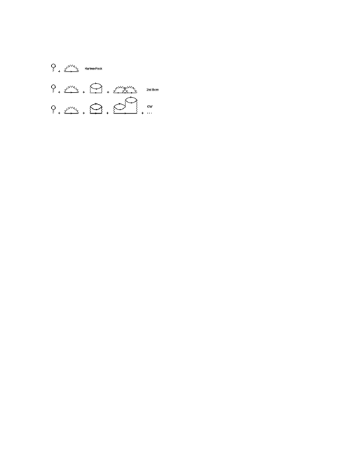
Baym has proven [27] that such $\Phi$-derivable or conserving approximations [28, 27, 29] automatically lead to satisfaction of the conservation laws provided that the equations of motion for the Green’s function are solved to full self-consistency. Commonly used conserving approximations for $\mbox{\boldmath$\Sigma$}^{\rm{MB}}_{\rm CC}[\mbox{\boldmath$\mathcal{G}$}_{\rm{CC}}]$ are the Hartree-Fock, second Born and GW approximations [15, 24, 30, 31] which are displayed diagrammatically in Fig.2.

Figure 2: Diagrammatic representation of the self-energies for the conserving many-body approximations used.

2.4 Time-dependent current

An equation for the time-dependent current flowing into the lead $\alpha$ can be derived from the time-derivative of the number of particles in lead $\alpha$ using the equation of motion for the lead Green’s function $\mbox{\boldmath$\mathcal{G}$}_{\alpha\alpha}$ [13]. This yields

$$I_{\alpha}(t)=2\textnormal{Re}\,{\rm Tr}_{\rm C}\left[\mbox{\boldmath$\mathcal{G}$}_{\rm C\alpha}^{<}(t,t)H_{\alpha C}\right].$$ (31)

If we insert the adjoint of Eq. (13) and extract the different components from the resulting equation using the conversion table in Ref.[23], the equation for the current becomes [13]

$$I_{\alpha}(t) = 2\textnormal{Re}\,{\rm Tr}_{\rm C}\left[\int_{t_{0}}^{t}d\bar{t}\,\mbox{\boldmath$\mathcal{G}$}_{\rm CC}^{<}(t,\bar{t})\mbox{\boldmath$\Sigma$}_{{\rm em},\alpha}^{A}(\bar{t},t)+\int_{t_{0}}^{t}d\bar{t}\,\mbox{\boldmath$\mathcal{G}$}_{\rm CC}^{R}(t,\bar{t})\mbox{\boldmath$\Sigma$}_{{\rm em},\alpha}^{<}(\bar{t},t)\right.$$ (32)

$$\left.-i\int_{0}^{\beta}d\tau\,\mbox{\boldmath$\mathcal{G}$}_{\rm CC}^{\rceil}(t,\tau)\mbox{\boldmath$\Sigma$}_{{\rm em},\alpha}^{\lceil}(\tau,t)\right].$$

The first two terms in this equation contain integrations over earlier times from $t_{0}$ to $t$ and take into account the nontrivial memory effects arising from the time-nonlocality of the embedding self-energy and the Green’s functions. Furthermore, the last integral over the imaginary track incorporates the initial many-body and embedding effects. Equation (32) provides a generalization of the widely used Meir-Wingreen formula [32, 33] to the transient time-domain [13].

2.5 Nonequilibrium spectral function

The nonequilibrium spectral function for real times is defined as

$$A(t,t^{\prime})=i\,{\rm Tr}_{\rm C}[\mbox{\boldmath$\mathcal{G}$}_{\rm CC}^{>}-\mbox{\boldmath$\mathcal{G}$}_{\rm CC}^{<}](t,t^{\prime})=\sum_{i\in C,\sigma}\langle\left\{\hat{d}_{i\sigma}(t),\hat{d}_{i\sigma}^{\dagger}(t^{\prime})\right\}\rangle.$$ (33)

where the brackets in the last term denote the anti-commutator. It is common to Fourier transform this function with respect to the relative time-coordinate $\tau=t-t^{\prime}$ for a given value of the average time $T=(t+t^{\prime})/2$. The spectral function in the new coordinates is then

$$A(T,\omega)=-{\rm Im}\int\frac{d\tau}{2\pi}\,e^{i\omega\tau}{\rm Tr}_{\rm C}[\mbox{\boldmath$\mathcal{G}$}_{\rm CC}^{>}-\mbox{\boldmath$\mathcal{G}$}_{\rm CC}^{<}](T+\frac{\tau}{2},T-\frac{\tau}{2})={\rm Re}\int\frac{d\tau}{2\pi}\,e^{i\omega\tau}A(T+\frac{\tau}{2},T-\frac{\tau}{2})$$ (34)

If the time-dependent external field becomes constant after some switching time, then also the spectral function becomes independent of $T$ after some transient period. In that case we will denote the spectral function by $A(\omega)$. The spectral function for a system in equilibrium has peaks at the addition and removal energies. In the nonequilibrium case this is less clear as one can, in general, not use a Lehmann expansion to prove this fact. However, for a system to which a bias is suddenly applied one can still show that the spectral function will contain peaks at the addition and removal energies from the various excited states of the biased system.

2.6 The density in the leads

The density in the leads can be obtained from the Green’s function $\mbox{\boldmath$\mathcal{G}$}_{\alpha\alpha}$. This Green’s function satisfies an equation of motion that can be obtained by projecting the equation (7) into the $\alpha\alpha$ region:

$$\begin{split}&\Bigl{\{}i\partial_{z}\mathbf{1}-\mathbf{H}_{\alpha\alpha}(z)\Bigr{\}}\mbox{\boldmath$\mathcal{G}$}_{\alpha\alpha}(z,z^{\prime})=\delta(z,z^{\prime})\mathbf{1}\,\,+\mathbf{H}_{{\alpha\rm C}}\mbox{\boldmath$\mathcal{G}$}_{\rm C\alpha}(z,z^{\prime}).\end{split}$$ (35)

Using the adjoint of (13) in (35) we have

$$\Bigl{\{}i\partial_{z}-\mathbf{H}_{\alpha\alpha}(z)\Bigl{\}}\mbox{\boldmath$\mathcal{G}$}_{\alpha\alpha}(z,z^{\prime}) = \delta(z,z^{\prime})\mathbf{1}+\int_{\gamma}d\bar{z}\mbox{\boldmath$\Sigma$}_{\rm{in},\alpha}(z,\bar{z})\mbox{\boldmath$g$}_{\alpha\alpha}(\bar{z},z^{\prime}),$$ (36)

where we defined the inbedding self-energy as

$$\mbox{\boldmath$\Sigma$}_{\rm{in},\alpha}(z,z^{\prime})=\mathbf{H}_{\alpha{\rm C}}\mbox{\boldmath$\mathcal{G}$}_{\rm{CC}}(z,z^{\prime})\mathbf{H}_{{\rm C}\alpha}.$$ (37)

Equation (36) can now be solved using Eq.(12). By taking the time arguments at $t_{\pm}$ we get

$$\mbox{\boldmath$\mathcal{G}$}_{\alpha\alpha}(t_{-},t_{+}) = \mbox{\boldmath$g$}_{\alpha\alpha}(t_{-},t_{+})+\int_{\gamma}d\bar{z}d\bar{\bar{z}}\mbox{\boldmath$g$}_{\alpha\alpha}(t_{-},\bar{z})\mbox{\boldmath$\Sigma$}_{\rm{in},\alpha}(\bar{z},\bar{\bar{z}})\mbox{\boldmath$g$}_{\alpha\alpha}(\bar{\bar{z}},t_{+}).$$ (38)

We see from Eq.(6) that from this equation we can extract the time-dependent spin occupation of orbital $i$ in lead $\alpha$ by taking $r=s=i\sigma\alpha$. The first term on the r.h.s. of Eq. (38) gives the density of uncontacted biased lead $\alpha$ and the second term gives a correction to the density induced by the presence of the correlated scattering region. In practice we first solve the Kadanoff-Baym equations for $\mbox{\boldmath$\mathcal{G}$}_{\rm{CC}}$ and then we construct the inbedding self-energy $\mbox{\boldmath$\Sigma$}_{\rm{in}}$ which is then used to calculate the time-dependent lead density according to (38).

2.7 Embedding self-energy

In this section we derive the expression for the embedding self-energy for the case of one-dimensional noninteracting tight-binding leads. From equation (15) we see that the embedding self-energy is given by

$$\mbox{\boldmath$\Sigma$}_{{\rm em},\alpha,kl}(z,z^{\prime})=\sum_{ij}^{\mathcal{N_{\alpha}}}V_{k,i\alpha}\mbox{\boldmath$g$}_{\alpha\alpha,ij}(z,z^{\prime})V_{j\alpha,l},$$ (39)

where $k$,$l$ label the sites in the central region and $i$,$j$ the sites in the lead $\alpha$. Furthermore, $\mathcal{N}_{\alpha}$ is the number of sites in the lead $\alpha$ (at the end of the derivation we take $\mathcal{N}_{\alpha}\rightarrow\infty$). We now express the biased lead Green’s functions using the eigenbasis of the biased lead Hamiltonian:

$$\mbox{\boldmath$g$}_{\alpha\alpha,ij}^{\lessgtr}(z,z^{\prime}) = \sum_{pq}^{\mathcal{N}_{\alpha}}U^{\alpha}_{ip}\tilde{\mbox{\boldmath$g$}}^{\lessgtr}_{\alpha\alpha,pq}(z,z^{\prime})U_{qj}^{\alpha\dagger},$$ (40)

where

$$\tilde{\mbox{\boldmath$g$}}_{\alpha\alpha,pq}^{<}(z,z^{\prime}) = i\delta_{pq}f(\epsilon_{p\alpha})e^{-i\int_{z^{\prime}}^{z}(\epsilon_{p\alpha}-\mu+U_{\alpha}(\bar{z}))d\bar{z}},$$ (41)

$$\tilde{\mbox{\boldmath$g$}}_{\alpha\alpha,pq}^{>}(z,z^{\prime}) = i\delta_{pq}(f(\epsilon_{p\alpha})-1)e^{-i\int_{z^{\prime}}^{z}(\epsilon_{p\alpha}-\mu+U_{\alpha}(\bar{z}))d\bar{z}},$$ (42)

are the lead Green’s functions in the eigenbasis of the leads with eigenvalues $\epsilon_{p\alpha}$. The columns of matrix $\mathbf{U}^{\alpha}$ represent these eigenstates in site basis. The function $f(\epsilon)=1/(e^{\beta(\epsilon-\mu)}+1)$ is the Fermi distribution function. Inserting Eqs.(41) and (42) into the definition of the embedding self-energy (39) and defining the function

$$\Gamma_{kl,\alpha}(\epsilon)=2\pi\sum_{ijp}^{\mathcal{N}_{\alpha}}V_{k,i\alpha}U^{\alpha}_{ip}\delta(\epsilon-\epsilon_{p\alpha})U_{pj}^{\alpha\dagger}V_{j\alpha,l}$$ (43)

we get an expression for the one-dimensional lead self-energy

$$\mbox{\boldmath$\Sigma$}_{{\rm em},\alpha,kl}^{<}(z,z^{\prime}) = ie^{-i\int_{z^{\prime}}^{z}U_{\alpha}(\bar{z})d\bar{z}}\int\frac{d\epsilon}{2\pi}f(\epsilon)\Gamma_{kl,\alpha}(\epsilon)e^{-i(\epsilon-\mu)(z-z^{\prime})},$$ (44)

$$\mbox{\boldmath$\Sigma$}_{{\rm em},\alpha,kl}^{>}(z,z^{\prime}) = ie^{-i\int_{z^{\prime}}^{z}U_{\alpha}(\bar{z})d\bar{z}}\int\frac{d\epsilon}{2\pi}(f(\epsilon)-1)\Gamma_{kl,\alpha}(\epsilon)e^{-i(\epsilon-\mu)(z-z^{\prime})}.$$ (45)

The remaining task is to evaluate the function $\Gamma_{kl,\alpha}(\epsilon)$. For a tight-binding (TB) chain we have

$$\epsilon_{p\alpha} = a^{\alpha}+2T_{\alpha}\cos(\phi_{p}),$$ (46)

$$U_{np}^{\alpha} = \sqrt{\frac{2}{\mathcal{N}_{\alpha}+1}}\sin(n\phi_{p}),$$ (47)

where $a^{\alpha}$ and $T_{\alpha}$ are the tight binding on-site and hopping parameters for the lead $\alpha$ and $\phi_{p}=\frac{p\pi}{\mathcal{N}_{\alpha}+1}$, $p=1...\mathcal{N}_{\alpha}\,,n=1...\mathcal{N}_{\alpha}$. We consider the case that the coupling Hamiltonian has nonzero elements only at the terminal points adjacent to the endpoints of the central region nanowire, that is when $i=j=1$. The function $\Gamma_{kl,\alpha}(\epsilon)$ then becomes

$$\Gamma_{kl,\alpha}(\epsilon)=2\pi V_{k,1\alpha}V_{1\alpha,l}\sum_{p=1}^{\mathcal{N}_{\alpha}}U^{\alpha}_{1p}\delta(\epsilon-\epsilon_{p\alpha})U_{p1}^{\alpha\dagger}.$$ (48)

Inserting Eqs. (47) into (48) and taking the $\mathcal{N}_{\alpha}\rightarrow\infty$ limit we obtain

$$\Gamma_{kl,\alpha}(\epsilon)=\frac{2V_{k,1\alpha}V_{1\alpha,l}}{|T_{\alpha}|}\sqrt{1-\left(\frac{\epsilon-a^{\alpha}}{2T_{\alpha}}\right)^{2}}\times\theta(2|T_{\alpha}|-|\epsilon-a^{\alpha}|).$$ (49)

From the definition of $\Gamma_{kl,\alpha}(\epsilon)$ we see that it describes the weighted density of states of the lead $\alpha$ as a function of the energy. Equation (49) then yields the expression for the 1D lead self-energy

$$\mbox{\boldmath$\Sigma$}_{{\rm em},\alpha,kl}^{<}(z,z^{\prime})=i\frac{V_{k,1\alpha}V_{1\alpha,l}}{\pi|T_{\alpha}|}e^{-i\int_{z^{\prime}}^{z}U_{\alpha}(\bar{z})d\bar{z}}\int_{a^{\alpha}-2|T_{\alpha}|}^{a^{\alpha}+2|T_{\alpha}|}d\epsilon f(\epsilon)\sqrt{1-\left(\frac{\epsilon-a^{\alpha}}{2T_{\alpha}}\right)^{2}}e^{-i(\epsilon-\mu)(z-z^{\prime})},$$ (50)

and the $\mbox{\boldmath$\Sigma$}_{{\rm em},\alpha,kl}^{>}$ component is obtained by simply replacing the $f(\epsilon)$ with $f(\epsilon)-1$. Furthermore, the $\lceil$,$\rceil$ and ”M” components are similarly obtained by considering the time-arguments on different parts of the Keldysh contour.

3 Numerical results

We now apply the KB approach to study the transport dynamics of a quantum wire consisting of 4 sites connected to left and right one-dimensional TB leads, see Fig. 1 A. The nearest neighbour hoppings in the leads are set to $T_{\rm L}=T_{\rm R}=-2.0$ and the on-site energy $a^{\alpha}$ is set equal to the chemical potential, $a^{\alpha}=\mu$, yielding a half-filling for the lead energy bands. The values for the coupling Hamiltonian are set to $V_{1,1L}=V_{4,1R}=-0.5$ and the central region sites have the on-site energies $h_{ii}=0$ and hopping parameters $h_{ij}=-1.0$ between nearest neighbour sites $i$ and $j$. The electron-electron interaction in the central region has the form $v_{ijkl}=v_{ij}\,\delta_{il}\delta_{jk}$ with

$$v_{ij}=\begin{cases}v_{ii}&i=j\\ \frac{v_{ii}}{2|i-j|}&i\neq j\end{cases}$$ (51)

where $v_{ii}=1.5$.

Figure 3: Left panel: Time-dependent right current $I(t)$ and dipole moment $d(t)$ for different self-energy approximations when a DC bias $U_{0}=1.4$ is applied to the leads. The inset shows the absolute value Fourier transform of the dipole moment. Right panel: Steady state spectral function $A(\omega)$.

Figure 4: Panel a): Dipole moment $d(t)$ corresponding to bias $U_{1}(t)$. The inset shows the absolute value of the Fourier transform of the dipole moment. Panel b): Time-dependent current flowing into the right lead (top panel) and the time-dependent bias $U_{1}(t)$ (bottom panel).

Figure 5: Panel a): Dipole moment $d(t)$ corresponding to bias $U_{2}(t)$. The inset shows the absolute value of the Fourier transform of the dipole moment. Panel b): Time-dependent current flowing into the right lead (top panel) and the time-dependent bias $U_{2}(t)$ (bottom panel).

The chemical potential is fixed between the highest occupied molecular orbital (HOMO) and lowest unoccupied molecular orbital (LUMO) levels of the isolated central region and has the value $\mu=2.26$. Furthermore, the inverse temperature is set to $\beta=90$ corresponding to the zero temperature limit. We use different time-dependent bias voltages. We consider a sudden switch on DC case of the form $U_{L}(t)=-U_{R}(t)=U_{0}\theta(t-t_{0})$ and periodic AC pulses $U_{L}(t)=-U_{R}(t)=U_{1,2}(t)$ of the forms

$$U_{1}(t) = \begin{cases}U_{0}&0\leq t<\frac{T_{0}}{2}\\ -U_{0}&\frac{T_{0}}{2}\leq t<T_{0}\\ \end{cases}\,\,\,\,\,\,\textnormal{(block bias)}$$ (52)

$$U_{2}(t) = \begin{cases}U_{0}&0\leq t<\frac{T_{0}}{2}\\ 0&\frac{T_{0}}{2}\leq t<T_{0}\\ \end{cases}\,\,\,\,\,\,\,\,\,\,\,\textnormal{(on-off bias)}$$ (53)

which for $t>T_{0}$ are periodically extended using $U(t+T_{0})=U(t)$. The time $T_{0}$ is the period of the complete bias cycle corresponding to oscillation frequency $\omega_{0}=2\pi/T_{0}$. In all cases we choose the amplitude of the bias voltage to be $U_{0}=1.4$ and for AC biases we set the period to be $T_{0}=40$ a.u. Finally, to study how the charge distributes along the chain after a bias voltage is switched on we calculate the time-dependent dipole moment

$$d(t)=\sum_{i=1}^{4}x_{i}\,n_{i}(t)$$ (54)

where the $x_{i}$ are the coordinates of the sites of the chain (with a lattice spacing of one), with origin halfway between sites 2 and 3, and $n_{i}(t)$ is the site occupation number.
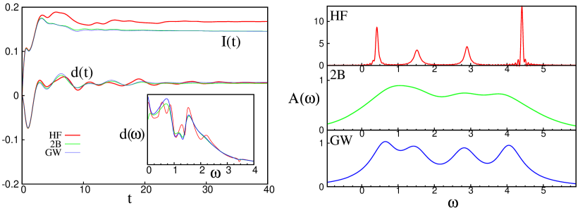
We start by considering the case of a suddenly switched DC bias. In the left panel of Fig. 3 we compare the time-dependent dipole moments (three lowermost curves) and transient currents (three uppermost curves) for the HF, 2B and GW approximations. The right panel shows the steady-state spectral functions. We see that the Hartree-Fock peaks are relatively sharp with a width approximately given by the imaginary part of the embedding self-energy at the Fermi level of $\Gamma=2V^{2}/T_{\alpha}\approx 0.25$ where $V=V_{1,1L}=V_{4,1R}$. On the other hand the 2B and GW spectral functions are very broadened due to strongly enhanced quasi-particle scattering at finite bias [26, 13]. We see that the Hartree-Fock approximation produces a slightly larger current compared to the 2B and GW approximations. This is in keeping with the fact that the HF spectral function integrated over the bias window leads to a slightly larger value as compared to those from the 2B and GW approximations. We further see that the correlated 2B and GW approximations lead to currents and dipole moments in close agreement with each other. This indicates that the dynamical screening of the Coulomb interaction as described by the first bubble diagram of the self-energy has a leading contribution.

In the inset of the left panel in Fig. 3 we display the absolute value of the Fourier transform of the dipole moment. We see a number of peaks that can be directly related to transitions from the lead electrochemical potentials $\mu+U_{\alpha}$ to the lead levels and between levels in the central sites themselves. The nature of these transitions can be deduced from the peak positions in the spectral function. Denoting these energies with $\Delta\epsilon_{Li}$, $\Delta\epsilon_{iR}$ and $\Delta_{ij}$ we can identify, at HF level, transitions at energies $\Delta\epsilon_{L3,2R}\approx 0.5$, $\Delta\epsilon_{L4}\approx 0.9$, $\Delta_{23}\approx 1.6$, $\Delta_{34}\approx 1.3$, $\Delta\epsilon_{L2,3R}\approx 2.25$ and $\Delta\epsilon_{L1,4R}\approx 3.3$. The largest peaks are due to the HOMO-LUMO transition $\Delta_{23}$ and the transitions $\Delta\epsilon_{L4}$, $\Delta\epsilon_{L3,2R}$ and we see that these are the only peaks that are clearly visible for the 2B/GW case, since in the correlated case the transients and dipole moments are strongly damped.

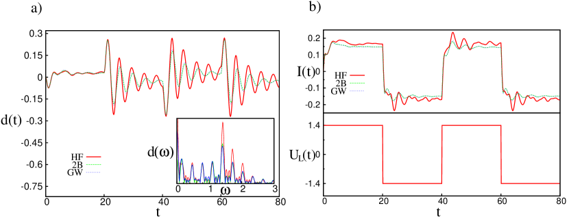
We now address the case of the AC block bias $U_{1}(t)$. In Fig. 4 we show the corresponding dipole moments and transient currents. As in the DC bias case we observe that the GW results are very close to the 2B results. The currents and dipole moments show a similar initial transient behavior as in Fig. 3 up to $t=20$ after which the bias switches sign. The inset in the Fig. 4 a) contains the Fourier transform of the dipole moment which displays peaks at the odd harmonics $(2n+1)\omega_{0}$ of the basic driving frequency $\omega_{0}$ of the AC bias. The appearance of odd harmonics is a consequence of the even inversion symmetry of the unbiased Hamiltonian and the odd inversion symmetry of the applied bias. We see up to 9 harmonic peaks which indicates that we are far from the linear response regime. From the inset of Fig. 4 we also see that the harmonics at energies $1.4$ (harmonic order 9) and $1.7$ (harmonic order 11) are enhanced. This is due to strong mixing with the HOMO-LUMO transition that occurs at energy 1.6 in the DC case (see fig.3).

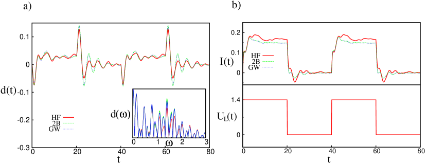
High harmonics with even order will develop when we break the symmetry of the unbiased Hamiltonian or of the applied bias. This happens for the case of the on-off AC bias voltage $U_{2}(t)$ (see Eq.(53)). The dipole moments and transients for this case are displayed in Fig. 5. The applied bias in this case has either even or odd inversion symmetry depending on the time interval considered. Therefore even harmonics at frequencies $2n\omega_{0}$ are also visible in the Fourier transform of the dipole moment (Fig. 5 inset). Also in this case the higher harmonics mix strongly with the main electronic transition frequencies leading to an increased intensity of the harmonics around the HOMO-LUMO gap frequency $\omega\approx 1.5$. Furthermore there are increased harmonic peaks at frequencies $\omega\approx 0.5,0.9$ which are due to mixing of the harmonics with the transitions $\Delta\epsilon_{L3,2R}$ and $\Delta\epsilon_{L4}$ (see fig.3).

Now we turn our attention to the spectral functions. In Fig. 6 we show the time-dependent spectral function $A(T,\omega)$ (per spin and shifted with the chemical potential $\mu$) for the HF and 2B approximations for the case of the on-off bias $U_{2}(t)$.

Figure 6: Time-dependent spectral function $A(T,\omega)$ in the HF (left panel) and 2B (right panel) approximation. The system parameters are the same as for Fig. 5.

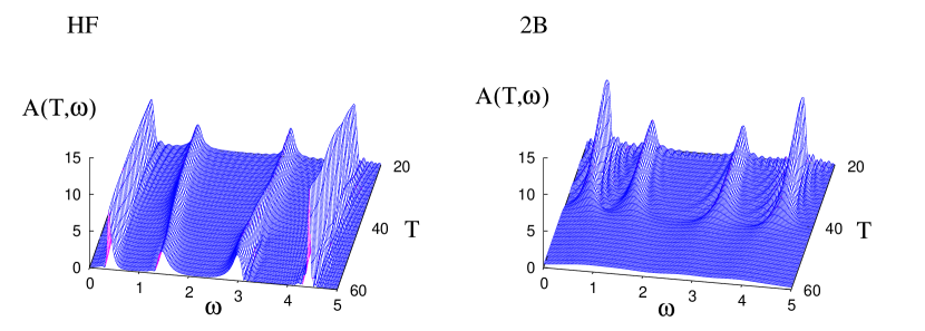
The system is first propagated without the external bias up to 40 a.u. after which the AC bias is turned on. We see that the spectral peaks in Hartree-Fock approximation remain sharp during the whole time-propagation and due to the applied bias a closing of the HOMO-LUMO gap takes place. In contrast to the HF approximation, the spectral peaks in 2B start to broaden and loose intensity rapidly after the bias has been switched on and is caused by enhanced quasiparticle scattering at finite bias.

Figure 7: Left panel: Real-time spectral function $A(t,t^{\prime})$ in the 2B approximation for on-off AC bias voltage. Right panel: The real and imaginary parts of $A(T+\tau/2,T-\tau/2)$ as a function of $\tau/2$ for T=70 (solid line) and T=90 (dashed line). The corresponding cross-sections are indicated with black lines.

Figure 8: Left panel: Real-time spectral function $A(t,t^{\prime})$ in the HF approximation for on-off AC bias voltage . Right panel: The real and imaginary parts of $A(T+\tau/2,T-\tau/2)$ as a function of $\tau/2$ for T=70 (solid line) and T=90 (dashed line). The corresponding cross-sections are indicated with black lines.

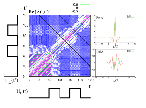
We note that we do not observe any noticeable shift in the position of the spectral peaks as a function of the alternating bias. This can be explained from an analysis of the spectral function $A(t,t^{\prime})$ in real time. We display contour plots of these functions in Figs. 7 and 8. In these figures we also display two center-of-time cross sections $A(T+\tau/2,T-\tau/2)$ for $T=70$ and $T=90$. Also for this case the ground state was first propagated without a bias up to 40 a.u. after which the AC field was switched on. Therefore for $t,t^{\prime}\leq 40$ the contour plot describes the equilibrium system. For such times the spectral function only depends on the relative time $t-t^{\prime}$. For $t,t^{\prime}>40$ the bias is applied and the spectral function starts to depend on both time-coordinates separately. This is especially visible for the 2B case in Fig.7 where for $40<t,t^{\prime}\lesssim 50$ we see a sudden collapse of the spectral function (we have checked this also for other values of the contour lines than displayed in the plot). This time interval coincides with the transient time of the current as shown in Fig.5. Note, however, that the spectral function $A(T,\omega)$ for average times $20<T\lesssim 30$ is still dominated by the equilibrium state since the Fourier transform over the relative time $\tau$ extends mainly over values of $t,t^{\prime}$ within the equilibrium region of the double time plane. For this reason the collapse of the spectral function $A(T,\omega)$ of Fig.6 occurs within the time interval from $T=20$ to $T=40$. In Fig. 7 we further observe a characteristic checkerboard pattern of the contour line at zero. This reflects the various combinations (on-on, on-off and off-off) of the functions $U_{2}(t)$ and $U_{2}(t^{\prime})$ at times $t$ and $t^{\prime}$. If we calculate the spectral function $A(T,\omega)$ by Fourier transforming over the relative time coordinate $\tau$ we make an average over these regions. This averaging makes the spectral function less sensitive to the period of the applied AC bias. Nevertheless, some periodic changes in the cross sections $A(T+\tau/2,T-\tau/2)$ can be observed. In the upper and lower right panels of Fig.7 we display these cross sections at average times $T=70$ (center of the off-period) and $90$ (center of the on-period) for both the real and the imaginary part of $A(T+\tau/2,T-\tau/2)$ as a function of $\tau/2$. On the time diagonal the real part of $A$ is always equal to $4$ since we have four states per spin in our atomic chain. Since the spectral function decays fast as a function of $\tau$ the main changes in the spectral function occur close to the time diagonal. When we Fourier transform these cross section small shifts in the spectral peaks are observed. In the on-state at $T=90$ we found a slight closing of the HOMO-LUMO gap as compared to the off-state at $T=70$.
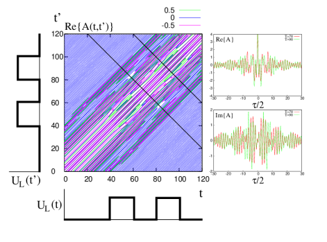
In Fig.8 we display the spectral function $A(t,t^{\prime})$ for the HF approximation. It can be seen that the oscillations along the relative time coordinate $\tau$ in the spectral functions are much less damped in HF (Fig. 8) than in 2B (Fig. 7). As a consequence we do not see the checkerboard pattern observed in the 2B case since it occurs much farther away from the time diagonal. The functions $A(T+\tau/2,T-\tau/2)$ clearly show a slow and a fast oscillation as a function of $\tau/2$ corresponding to the two outer and inner peaks (at positive and negative frequencies) of the time-dependent spectral function $A(T,\omega)$ displayed in Fig. 6. Note that in this figure we shifted the peaks with the chemical potential $\mu=2.26$.

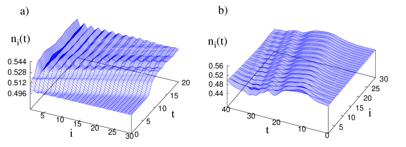
We now turn our attention to the lead densities for the case of the AC block bias $U_{1}(t)$. In right/left panel of Fig. 9 we show the time evolution of the site occupation numbers $n_{i}(t)$ in the right lead for the AC/DC biases. These are calculated for up to 30 sites deep into the lead from Eq.(38) using $n_{i}(t)=-i\mbox{\boldmath$\mathcal{G}$}_{\alpha\alpha,rr}(t_{-},t_{+})$ where $r=i\sigma$. For the case of a DC bias shown in panel (a) we can clearly observe a density wave front that propagates into the right lead. Furthermore the electron density displays a zigzag-pattern with an amplitude that decreases away from the first site into the lead. These are the usual Friedel oscillations caused by the presence of the atomic chain in the lattice. Their spatial profile is given by $\delta n(x)\sim\sin(2k_{F}x)$ where $k_{F}$ is the Fermi wave vector and $x$ the distance to the impurity site. In the case of the half-filled lead energy band that we consider $k_{F}=\pi/2$ corresponding to a density variation that alternates on every site. When we switch on the bias in the leads the Friedel oscillations get enhanced by roughly an order of magnitude.

In panel (b) of Fig.9 we shown the lead density profile for the case of the AC bias $U_{1}(t)$. As in the DC case, we see a wavefront moving into the lead. However, due to the periodic alternation of the bias these wavefronts get superimposed on the returning ones giving rise to interferences causing additional wiggles in the density profile.

Figure 9: Site occupation number $n_{i}(t)$ per spin in the right lead as a function of time $t$ and site label $i$. The results are displayed for (a) DC bias, and (b) AC bias $U_{1}(t)$ within the HF approximation.

4 Conclusions

We proposed a time-dependent many-body approach based on the real time propagation of the KB equations for open and inhomogeneous systems.

The method was applied to study transport dynamics through an atomic chain under AC and DC bias voltages. We calculated the spectral functions and the time-dependent current, density and dipole moment within the HF, second Born and GW conserving approximations. We found that electron correlations beyond mean field have a large impact on time-dependent and steady state properties. Both in the AC and DC case the HF spectral function retains its sharp structures upon applying a bias, while the spectral function calculated within the 2B and GW approximations broadens considerably.

The strong AC biases that we applied lead to highly nonlinear perturbations. As a consequence high-order harmonics of the driving frequency are observed in the time-dependent dipole moment. Depending on the symmetry of the Hamiltonian and of the applied AC voltage the odd and even harmonics are generated. The harmonics with largest intensity are those with energy close to the HOMO-LUMO gap.

References

- [1] R. H. M. Smit et al, Nature 419, 906-909 (2002).
- [2] M. A. Reed et al, Science Vol. 278. no. 5336, 252-254 (1997).
- [3] L. P. Kouwenhoven, A. T. Johnson, N. C. van der Vaart, C. J. P. M. Harmans, and C. T. Foxon, Phys. Rev. Lett. 67, 1626 (1991).
- [4] M. Switkes, C. M. Marcus, K. Campman, and A. C. Gossard, Science 283, 1905 (1999).
- [5] P. J. Leek, M. R. Buitelaar, V. I. Talyanskii, C. G. Smith, D. Anderson, G. A. C. Jones, J. Wei, and D. H. Cobden, Phys. Rev. Lett. 95, 256802 (2005).
- [6] Z.Zhong, N.M.Gabor, J.E.Sharping, A.L.Gaeta, and P.L. McEuen Nature Nanotechnology 3, 201 (2008)
- [7] A.Tikhonov, R.D.Coalson, and Y.Dahnovsky J.Chem.Phys. 117, 567 (2002)
- [8] R.Baer, T.Seideman, S.Ilani, and D.Neuhauser J.Chem.Phys. 120, 3387 (2004)
- [9] V.Moldoveanu, V.Gudmundsson and A.Manolescu Phys.Rev.B 76, 165308 (2007)
- [10] V. Moldoveanu, A. Manolescu, V.Gudmundsson, cond-mat arXiv:0909.0815.
- [11] G. Stefanucci, S. Kurth, A. Rubio and E. K. U. Gross, Phys. Rev. B 77, 075339 (2008).
- [12] P. Myöhänen, A. Stan, G. Stefanucci and R. van Leeuwen, Europhys. Lett. 84, 67001 (2008).
- [13] P. Myöhänen, A. Stan, G. Stefanucci and R. van Leeuwen, Phys. Rev. B 80, 115107 (2009).
- [14] N. E. Dahlen, A.Stan and R.van Leeuwen J. Phys. Conf. Ser. 35, 324 (2006).
- [15] N. E. Dahlen and R. van Leeuwen, Phys. Rev. Lett. 98, 153004 (2007).
- [16] M. Puig von Friessen, C. Verdozzi, and C.-O. Almbladh, condmat arXiv:0905.2061.
- [17] K. Balzer, M. Bonitz, R. van Leeuwen, N. E. Dahlen and A. Stan, Phys. Rev. B 79, 245306 (2009).
- [18] L. P. Kadanoff and G. Baym, Quantum Statistical Mechanics (Benjamin, New York, 1962).
- [19] P. Danielewicz, Ann. Phys. (N.Y.) 152, 239 (1984).
- [20] N.-H. Kwong and M. Bonitz Phys. Rev. Lett. 84, 1768 (2000).
- [21] M. Wagner, Phys. Rev. B 44, 6104 (1991).
- [22] G. Stefanucci and C.-O. Almbladh, Phys. Rev.B 69, 195318 (2004).
- [23] R. van Leeuwen, N. E. Dahlen, G. Stefanucci, C. O. Almbladh, and U. von Barth, Time-Dependent Density Functional Theory (Springer, New York, 2006); Lect. Notes Phys. 706, 33 (2006).
- [24] A. Stan, N. E. Dahlen and R. van Leeuwen, J. Chem. Phys. 130, 224101 (2009).
- [25] K. S. Thygesen and A. Rubio Phys. Rev. B77, 115333 (2008).
- [26] K. S. Thygesen, Phys. Rev. Lett. 100, 166804 (2008).
- [27] G. Baym Phys. Rev. 127, 1391 (1962).
- [28] G. Baym and L. P. Kadanoff, Phys. Rev. 124, 287 (1961).
- [29] U. von Barth, N. E. Dahlen, R. van Leeuwen and G. Stefanucci, Phys. Rev. B 72, 235109 (2005).
- [30] A. Stan, N. E. Dahlen and R. van Leeuwen, J. Chem. Phys. 130, 114105 (2009).
- [31] N. E. Dahlen and R. van Leeuwen, J. Chem. Phys. 122, 164102 (2005).
- [32] Y. Meir and N. S. Wingreen, Phys. Rev. Lett. 68, 2512 (1992).
- [33] A.-P. Jauho, N. S. Wingreen and Y. Meir, Phys. Rev. B 50, 5528 (1994).