Visible Effects of Invisible Hidden Valley Radiation
Abstract:
Assuming there is a new gauge group in a Hidden Valley, and a new type of radiation, can we observe it through its effect on the kinematic distributions of recoiling visible particles? Specifically, what are the collider signatures of radiation in a hidden sector? We address these questions using a generic -like Hidden Valley model that we implement in Pythia. We find that in both the and the LHC cases the kinematic distributions of the visible particles can be significantly affected by the valley radiation. Without a proper understanding of such effects, inferred masses of “communicators” and of invisible particles can be substantially off.
MCnet/10/11
1 Introduction
One common feature in New Physics models is the conservation (or near conservation) of a new quantum number. Often it is associated with a parity symmetry, like R-parity in supersymmetric models or T-parity in Little Higgs ones. Such conserved parity-like symmetries serve two basic model-building purposes: firstly, they forbid odd-parity tree level corrections to electroweak precision observables, and secondly, they make the lowest lying odd-parity state stable, thus providing a possible dark matter candidate. The new charge may alternatively come from a continuous symmetry, a global symmetry or a new gauge symmetry, for example, and still fulfill the same purposes.
Regardless of the specific model realization, we can imagine that a new conserved quantum number is discovered at LHC.
In this article, we wish to take some first steps towards addressing a general phenomenological question: if a new apparently conserved charge should be discovered, is it possible to determine experimentally whether it arises from a discrete, a global or a gauge symmetry? Specifically, is it possible to determine whether it is the source of a new field?
In principle, a continuous symmetry has additive quantum number conservation whereas a discrete one has multiplicative conservation. To distinguish between gauge and global symmetries one could look for Gauge bosons, for Goldstone bosons and in general at the particle spectrum. The new sector however may be ”hidden”. That is, the carriers of the new symmetry, for the two basic reasons mentioned above, could lie entirely within the new sector and be neutral under (or have very weak) SM interactions. Indeed, a new unbroken symmetry would have to be invisible or else it would have already been found. Thus any radiation or other dynamic phenomena associated with it would be invisible to SM matter.
If the charge did radiate in the new sector, would we be still be able to observe indirectly the effects of the hidden radiation? How would the kinematic distributions of the visible particles be affected? Could we extract information from these kinematic distributions about the dynamics within the hidden sector? Could one distinguish Abelian from non-Abelian gauge groups, study the different particle (or unparticle) contents or measure the strength of the couplings? This could lead to a better understanding of the higher-energy dynamics, the ultraviolet completion of the theory, the symmetries involved, and possibly even the mechanism by which they are broken.
The ideal terrain to begin to explore these effects is Hidden Valley models [1]. We extend this name to the class of models satisfying the following criteria. First, there must be a new light hidden sector (the valley), decoupled from the visible SM one, that has not yet been discovered because of some barrier. This can be an energy barrier or of another nature, e.g. symmetry-forbidding tree-level couplings. Second, the decoupling of the new hidden valley sector from the visible SM one must happen at relatively low energies, around the TeV scale, in such a way that the cross sections for Standard visible particles disappearing into the hidden sector (and vice versa) are small enough to evade the current experimental limits, and yet large enough to be observable at LHC. These experimental limits are of course model dependent, as we will discuss in sections 2 and 4.
Typically, the valley particles ”v-particles” are charged under a valley group and neutral under the SM group , and the SM particles are neutral under . In order to have interactions between the two sectors there has to be a ”communicator” which couples to both SM and valley particles. A common choice is to have a coupling via a or via loops of heavy particles carrying both and charges.
Examples of Hidden Valleys can be found in many models, such as String Theory [3], Twin Higgs models [4], folded SUSY [5, 6], and Unparticle models [2, 7].
Hidden Valley scenarios can naturally provide candidates for Dark Matter and can easily fit cosmological constraints. Just to give an example, in [1] the v-interactions ensure that all particles efficiently decay to the lightest mesons. These mesons are allowed to annihilate to neutral s, which can then tunnel back into the SM. So long as the lifetime of the is sec, the number of s left will decay exponentially before big-bang nucleosynthesis.
The reason why these scenarios are ideal to study the effects of radiation is the large disparity in the masses of the communicators and the v-particles. Typically, the communicator has a mass around the decoupling scale, say the TeV scale, while the v-particle mass may be as low as 1–10 GeV. If both the communicator and the v-particle are charged under a new gauge , they will radiate gauge bosons, and the larger their mass ratio the larger the amount of phase space available for the radiation, both in the normal and in the hidden sector. Thus if any effect at all are to be observable, it would be in this kind of scenario.
We have devised a Hidden Valley toy model to tackle the issue, and have implemented it in the Pythia 8 Monte Carlo event generator [9]. The implementation allows for different valley flavour contents, particle masses, gauge groups and v-gauge couplings. In this way one may accommodate a range of different Hidden Valley scenarios.
MC event generators offer flexible approaches to model radiation and parton shower evolution in great detail. One new central feature in the Pythia 8 implementation is the “competition” mechanism between the hidden and the SM radiation, which is implemented as an “interleaved” shower, wherein different kinds of emissions, SM and hidden, can alternate if viewed in terms of a common shower evolution scale. As a consequence, subsequent emissions in the visible sector, of gluons or photons, will then tend to have a lower energy than they would have had, had the hidden radiation not been there. This is the key mechanism whereby we gain access to the information about the radiation in the hidden sector.
The intention of this article is not a full-fledged experimental analysis of how a new sector should be discovered and explored, neither with respect to potential background processes nor to detector-specific capabilities — since our implementation is publicly available, we safely leave it to the experimental community to assess. What we want to ascertain here is if there are observable signals of hidden valley radiation at all, at the simple parton and hadron levels.
It is not trivial to decide which visible particle kinematic distributions one should study to reveal valley radiation effects and to discriminate between different models. For instance, at an collider the rise of the communicator pair-production cross section near threshold could allow to determine its spin, and thereafter the absolute size of the cross section could suggest the presence of new “colour” factors — recall that the pair-production of particles in the fundamental representation of a new group gives a factor in the cross section. Such measurements would not directly probe the hidden sector, however: they would not reveal whether a new group is gauged, or what is the coupling strength in it. For a hadron collider, like the LHC, the uncertainty in the event-by-event subcollision energy undermines analyses solely based upon the value of cross-section. The best strategy is thus to complement cross-section with invariant mass measurements and the study of other boost-invariant quantities (for a recent review see the proceedings [16]).
This is the reason why we choose to study MT2 [15] distributions, which give relations between communicator and v-particle mass. These observables are specifically designed to be boost-invariant and to deal with BSM models in which more than one particle escapes detection, such as in our toy model. But we also study ”hidden observables”, like the invariant mass distribution of a hidden particle together with its associated hidden radiation.
The effects of the hidden radiation on these distributions and how much one may observe depends on the details of the scenario considered, of course, but also depend heavily upon the collider type considered, on its center of mass energy, and on its integrated luminosity . We consider two different LHC scenarios, one for the early data (the first 18 to 24 months at TeV with an expected integrated luminosity fb-1) and one for later data ( TeV and integrated luminosity fb-1). The conclusions in the two cases will be quite different. For collisions we will mainly refer to an ILC at 800 GeV, though we mention CLIC production cross sections at 3 TeV.
The paper is organized as follows: we give a first overview of the various valley scenarios in the literature, in section 2, and then describe the tools that are now available in Pythia in section 3. In section 4 we explain the model and the main features of interleaved SM and hidden radiation. Finally, in the last two sections we study the effects of hidden radiation on collider phenomenology. In section 5 we discuss the case and in section 6 the LHC one.
2 Hidden Valley scenarios
As mentioned in the introduction a Hidden Valley is a light hidden sector, consisting of particles which, depending on the model, might have masses as low as GeV. The detailed spectrum of the v-particles and their dynamics within the hidden valley depends upon the valley gauge group , the spin and number of particles present in the theory, and the representation they belong to.
The effects of the hidden sector on the visible particle spectra will depend upon the way the hidden sector communicates with the SM, whether it is via a Higgs, multiple Higgses, a , heavy sterile neutrinos or via loop of heavy particles charged under both SM and valley gauge interactions.
We would like to give a panoramic view of the different Hidden Valley scenarios without going into details and to underline those features that may be simulated with the new tools.
The simplest possibility is a QCD-like scenario, with a strong coupling constant, which may run like the QCD coupling does, with QCD-like hadronization generating valley pions, v-s, v-s, v-nucleons etc. The Standard Model sector could couple ultra-weakly with the hidden sector via a neutral . This scenario was investigated by Strassler and Zurek with tools analogous to the ones used to simulate QCD [1]. It displays some rather startling features. For instance, a v- could have a displaced decay in the muon spectrometer in the ATLAS detector, resulting in a large number of charged hadrons traversing the spectrometer, or it could decay in the hadronic calorimeter producing a jet with no energy deposited in the electromagnetic calorimeter and no associated tracks in the inner detector. Experimental studies for these scenarios are currently under way, by the D0, CDF, LHCb, ATLAS and CMS collaborations.
Typical hidden valley-like signatures appear also in Unparticle models with mass gaps [7]. These models display a conformal dynamic above the mass gap, and a hidden valley behaviour when the conformal symmetry is broken. Regardless of the dynamics above the mass gap, whether it is strongly coupled or weakly coupled, the signatures are similar to the ones mentioned in the previous scenario (displaced vertices and missing energy signals). This is because only the lower energy states, light stable hidden hadrons can decay back into Standard Model particles. The higher energy states, be they narrow resonances or a continuum of resonances, decay rapidly to these lower light stable hadrons. As for the previous scenario, a parton shower is a key tool to study these models, not so much to determine the phenomenology qualitatively, but because it the only element of the hidden dynamics which is sensitive to the higher-energy conformal (or next-to-conformal) dynamics. The conformal dynamics will be reflected in the parton shower evolution, which can be rather different from the regular QCD one, especially in theories with a strong dynamics above the mass gap.
There are of course many other Hidden-Valley related models, such as Quirky models [8], just to give an example, in which the parton shower evolution does not play the key role it does in the previous cases. Typically their phenomenology is better captured in terms of string dynamics and string fragmentation.
In this paper we do not address the issue of string fragmentation or hadronization. Our main focus is on the parton shower, as this best captures the nature of the hidden radiation.
The model we built to investigate the existence of a this new radiation exploits but a few features common in many hidden valley scenarios: the presence of a new unbroken hidden gauge group, of a heavy communicator, charged under both SM and hidden sector gauge group and decaying into a visible and an invisible light particle, charged only under the new gauge group. These characteristics fit many Hidden Valley models, we however make an additional assumption, which is that the production cross sections111We will discuss the production cross sections in section 4. should be large enough for the effects of the hidden radiation to be discernable. This model was then implemented in the Pythia event generator. Notice however, that the shower mechanism we implemented is rather different from the ones mentioned above, as we will discuss in the next section.
3 Monte Carlo Tools in PYTHIA 8
In order to allow detailed studies of a set of scenarios, the models have been implemented in the Pythia event generator, and will be publicly available from version 8.140 onwards.
3.1 Particle content
For simplicity we assume that the HV contains either an Abelian or a non-Abelian gauge group, with spin 1 gauge bosons. The former group could be unbroken or broken, while the latter always is assumed unbroken. Casimir constants could be generalized to encompass other gauge groups, should the need arise, but for now we do not see that need. The gauge bosons are called and , respectively.
A particle content has been introduced to mirror the Standard Model flavour structure. These particles, collectively called , are charged under both the SM and the HV symmetry groups. Each new particle couples flavour-diagonally to a corresponding SM state, and has the same SM charge and colour, but in addition is in the fundamental representation of the HV colour, see Table 1. Their masses and widths can be set individually. It would also be possible to expand the decay tables to allow for flavour mixing.
| name | partner | code | name | partner | code |
|---|---|---|---|---|---|
| 4900001 | 4900011 | ||||
| 4900002 | 4900012 | ||||
| 4900003 | 4900013 | ||||
| 4900004 | 4900014 | ||||
| 4900005 | 4900015 | ||||
| 4900006 | 4900016 | ||||
| 4900021 | |||||
| 4900022 | |||||
| 4900101 |
These particles can decay to the corresponding SM particle, plus an invisible, massive HV particle , that then also has to be in the fundamental representation of the HV colour: . The notation is intended to make contact with SM equivalents, but obviously it cannot be pushed too far. For instance, not both and can be fermions. We allow the to have either of spin 0, and 1. Currently the choice of spin is not important but, for the record, it is assumed to be spin if the is a boson and either of spin 0 and 1 if is a fermion.
3.2 Production processes
The HV particles have to be pair-produced. The production processes we have implemented are the QCD ones, and , for the coloured subset of states, and the electroweak for all states. All of them would contribute at a hadron collider, but for a lepton one only the latter would be relevant. Each process can be switched on individually, e.g. if one would like to simulate a scenario with only the first generation.
Note that pair production cross sections contain a factor of , with for an group, for the pair production of new particles in the fundamental representation of the HV gauge group, in addition to the ordinary colour factor for . Other things equal, this could be used to determine from data, as already discussed. For the case of a spin 1 it is possible to include an anomalous magnetic dipole moment, .
The spin structure of the decay is currently not specified, so the decay is isotropic. Also the Yukawa couplings in decays are not set as such, but are implicit in the choice of widths for the states.
The kinematics of the decay is strongly influenced by the mass. This mass is almost unconstrained, and can therefore range from close to zero to close to the masses. We will assume it is not heavier than them, however, so that we do not have to consider the phenomenology of stable particles.
3.3 Parton showers
Both the and the can radiate, owing to their charge under the new gauge group, i.e. and for a group, and and for a one. In the latter case also non-Abelian branchings are allowed. Currently both and are assumed massless, but a broken with a massive is foreseen.
These showers form an integrated part of the standard final-state showering machinery. Specifically, HV radiation is interleaved with SM radiation in a common sequence of decreasing . That is, at the stage before the ’s decay, they may radiate , and , in any order. For the ’th emission, the evolution starts from the maximum scale given by the previous emission. The overall starting scale is set by the scale of the hard process. Thus the probability to pick a given takes the form
| (1) |
where the exponential corresponds to the Sudakov form factor. Implicitly one must also sum over all partons that can radiate.
To be more precise, radiation is based on a dipole picture, where it is a pair of partons that collectively radiates a new parton. The dipole assignment is worked out in the limit of infinitely many (HV or ordinary) colours, so that only planar colour flows need be considered. Technically the total radiation of the dipole is split into two ends, where one end acts as radiator and the other as recoiler. The recoiler ensures that total energy and momentum is conserved during the emission, with partons on the mass shell before and after the emission. In general the dipoles will be different for QCD, QED and HV.
To take an example, consider , which proceeds via an intermediate -channel gluon. Since this gluon carries no QED or HV charge it follows that the pair forms a dipole with respect to these two emission kinds. The gluon does carry QCD octet charge, however, so do not form a QCD dipole. Instead each of them is attached to another parton, either the beam remnant that carries the corresponding anticolour or some other parton emitted as part of the initial-state shower. This means that QCD radiation can change the invariant mass of the system, while QED and HV radiation could not. When a or is emitted the dipole assignments are not modified, since these bosons do not carry away any charge. A or would, and so a new dipole would be formed. For QCD the dipole between and one beam remnant, say, would be split into one between the and the , and one further from the to the remnant. For HV the dipole would be spit into two, and . As the shower evolves, the three different kinds of dipoles will diverge further.
Note that, in the full event-generation machinery, the final-state radiation considered here is also interleaved in with the initial-state showers and with multiple parton-parton interactions.
There is made a clean separation between radiation in the production stage of the pair and in their respective decay. Strictly speaking this would only be valid when the width is small, but that is the case that interests us here. In the decay the QCD and QED charges go with the and the HV one with . For all three interactions the dipole is formed between the and the , so that radiation preserves the system mass, but in each case only the relevant dipole end is allowed to radiate the kind of gauge bosons that goes with its charge. (Strictly speaking dipoles are stretched between the or and the “hole” left behind by the decaying . The situation is closely analogous to decays.)
The HV shower only contains two parameters. The main one is the coupling strength , i.e. the equivalent of . This coupling is taken to be a constant, i.e. no running is included.
From a practical point of view it is doubtful that such a running could be pinned down anyway, and from a theory point of view it means we do not have to specify the full flavour structure of the hidden sector. The second parameter is the lower cutoff scale for shower evolution, by default chosen the same as for the QCD shower, GeV.
The HV showers are not matched onto higher-order matrix elements for the emissions of hard in the production process, and so contain an element of uncertainty in that region. For the decay process the matching to first-order matrix elements have been worked out for all the colour and spin combinations that occurs in the MSSM [13], and is recycled for the HV scenarios, with spin 1 replaced by 0 for non-existing (in MSSM) combinations. This means that the full phase space is filled with (approximately) the correct rate. Some further approximations exists, e.g. in the handling of mass effects in the soft region. The chosen behaviour has been influenced by our experience with QCD, however, and so should provide a good first estimate. More than that we do not aim for in this study.
4 The model: SM and radiation
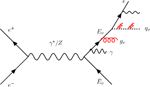
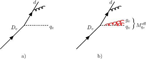
To be specific, in the following we explore two similar Hidden Valley experimental scenarios. In the first, the communicator is a spin 1/2 particle charged under both the SM and the valley gauge group . We assume it has the same SM charges an electron would have, so it may be pair-produced in collisions, via . Under the unbroken , it transforms like a , so it radiates both s and massless hidden valley gluons s. After the parton shower, the eventually decays into a visible SM electron and an invisible spin 0 valley “quark” . This belongs to the fundamental representation of and is not charged under the SM gauge group, so it only radiates s. See Fig. 1.
The key feature is interleaved radiation, already introduced above. In the current context it works as follows. Once the has been produced it may radiate a SM , say. This radiation will subtract energy from the and the following emission, be it another SM photon or a valley gluon, will have less phase space to radiate into. In an analogous way, assuming a valley is emitted next, it subtracts energy from and affects the following emissions which, again, could be either visible or invisible.
In the second scenario the communicator between SM sector and Hidden Valley sector is a quark-like, spin 1/2 object , belonging to the representation of the gauge group . The s are pair produced (mostly) via strong interactions (gluon-gluon or fusion). We choose the scenario in which only one vector-like is produced, the . This emits massless valley gluons (since the is assumed to be unbroken) and these may in turn radiate more s. During the shower evolution, both types of gluons are radiated until finally each decays into a visible SM quark an invisible spin 0 valley . The decays are flavour diagonal, .
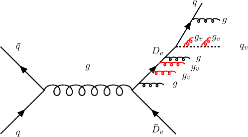
The SM quark transforms as a under , so it radiates only SM gluons, while the valley belongs to the representation of , so not having any SM color charge, it radiates only s., see figure 2.
In both scenarios there are just three parameters left to vary: the size of the valley coupling constant , the masses of the communicator particles or and the mass of the valley scalar .
Below, in Table 2, we list the total production cross sections at different colliders: with GeV or TeV, and LHC with TeV or TeV for some typical mass values.
| ILC | CLIC | LHC | LHC | ||
|---|---|---|---|---|---|
| (800 GeV) | (3 TeV) | (7 TeV) | (14 TeV) | ||
| GeV | 398 fb | 44 fb | GeV | fb | fb |
| GeV | - | 41 fb | GeV | 654 fb | fb |
| TeV | - | 32 fb | TeV | 3.21 fb | fb |
We also show the spin dependence of the production cross section at colliders for the three cases: spin 0 and spin 1/2, spin 1/2 and spin 0 or 1, and spin 1 and spin 1/2, Fig. 3.
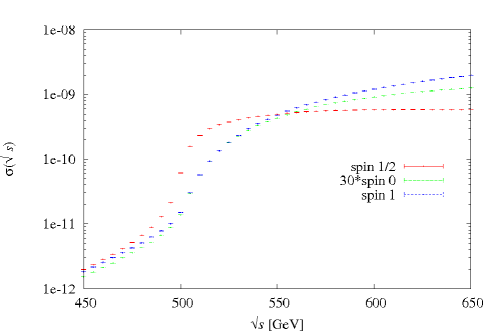
The higher the spin, the larger the cross section. Indeed, the curve corresponding to spin 0 has been scaled by a factor 30 to emphasize the similarity in shape with the spin 1 curve. Note that the processes proceed through the -channel exchange of a spin 1 . Thus the production of a spin pair has only a threshold factor from phase space, where is the velocity of the produced pair in the decay vertex, while the other two have an (approximate) additional factor from helicity considerations. The results have again been obtained with a group, and are directly proportional to the chosen. Since we would not expect gauge groups with above (some multiple of) 30, the conclusion would be that a threshold scan of the cross section could be used to determine both the spin and the number of hidden colours, as well as the mass, of course. A caveat would be that we have here only considered the gauge production mechanism, not the possibility of a significant channel Yukawa contribution. The reason for not including this production channel is that it would imply a large decay width for the , which would give additional large and model dependent effects to the cross section around threshold (see below).
The experimental constraints on these two types of setup are similar to the ones for New Charged Leptons and Leptoquark production222We do not make use of the limits coming from the D0 or CDF searches, because these depend upon the chosen mSUGRA scenario.. For the New Charged Leptons the PDG [10] gives the lower bound GeV. For scalar and vector Leptoquark states we use the direct limits coming from leptoquark pair production and subsequent decay searches [11]. For the all generation search GeV in the scalar case and GeV in the vector case, where one assumes the branching ratio . Bounds on the leptoquark mass for the third generation decaying into are more stringent [12], GeV.
We view these boundaries as simply indicative of the mass range we should contemplate and chose masses that are well beyond these boundaries. Our studies are in any case not critically dependent on them.
We assumed the communicators to be massive, in the range [250,300] GeV for the ILC case, in the range [300, 500] GeV for the LHC 7 TeV run, and [0.5,1] TeV for the 14 TeV run. The hidden scalar is taken to be light, as light as 10 GeV. The parameter is allowed to vary over a wide range, and results shown for interesting values.
Depending on the size of these parameters, the effects of the radiation on the lepton or quark kinematic distributions can be significant, as we will show in the next two sections. But whether these effects will be observable strongly depends on the statistics at hand. We assume an integrated luminosity fb-1 for the ILC, 1 fb-1 for the 7 TeV LHC run and 100 fb-1 for the 14 TeV one.
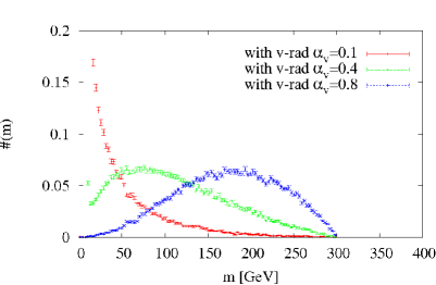
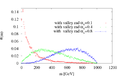
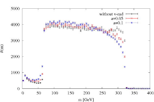
The hidden radiation affects the visible particle kinematics through two mechanisms. The first one, interleaved radiation from the or , we already discussed. The second is radiation off the after decay. This causes the invariant mass for the system made out of and the radiated s to be larger than the on-shell mass. This invariant mass can be viewed as the off-shell mass with which the is produced at the decay vertex. In Fig. 4 one may see the effects of the valley radiation on the off-shell mass, for the case. As the hidden valley coupling increases, the radiates more and more into the hidden sector, and the mean value of the distribution shifts from towards . At the same time more and more energy is subtracted from the visible recoiling particle, in this case the and its system of emitted gluons.
The effect is more obvious when the mass difference is large, since more phase space is available for the radiation.
The size of the deviations induced by these two combined mechanisms is very much dependent on the collider, as we already stressed above. In the next two sections we will discuss the various cases separately.
5 Effects of radiation at colliders
We begin by studying the , scenario, which allows for many simplifications compared to the quark case, and therefore offers a convenient warmup. For the ILC with GeV and an assumed integrated luminosity of fb-1 per year an GeV translates into about 80000 pairs.
5.1 Collisions in the center-of-mass frame
To illustrate the principles, as a very first step we will neglect bremsstrahlung and beamstrahlung. We then only need to consider two types of interactions, electromagnetic and valley radiation in the final state, with coupling constants and . No fragmentation or hadronization need to be taken into account.
Since the center of mass (CM) of the collision is at rest, there is a clean relationship between the mass of the hidden valley , , and that of the communicator . In the absence of radiation (hidden or standard), this can be inferred from the distribution of the energy of the emitted electrons, in particular from the upper endpoint of this distribution, describing the electron maximum energy. This is obtained when the electron is emitted in the same direction as the is moving in, with the in the opposite direction. One may use this maximization condition to derive the relationship between and .
In the rest frame of the , neglecting the electron mass,
| (2) | |||||
Assuming the boost to the CM rest frame is at an angle with respect to the direction in the rest frame, the electron energy will be given by
| (3) |
where gives the upper and lower edge of the energy spectrum. If the decay is assumed isotropic, constant, the electron energy spectrum is flat between the limits.
So if one can measure the maximum and minimum energy , one may solve for and . Fig. 6 shows the energy distribution of the electrons produced with and without hidden radiation. In the latter case the spectrum is shifted to lower values, as the hidden sector takes a bigger fraction of the available energy, by radiation off both the and the . The endpoints remain the same, as there is always a fraction of events where radiation is negligible. As we have assumed a modest width of 1 GeV for the there is a tiny tail beyond the expected edge. (We could cope with a wide range of widths, but have picked values in the GeV range, so that the possibility of a Breit-Wigner-shaped mass broadening is not overlooked, while still maintaining a credible simulation in terms of resonance diagrams only.) The key point to observe, however, is how the upper “shoulder” is softened by the hidden radiation. Thereby a precision measurement of this region would offer a direct check on the amount of hidden radiation. At the lower end, QED cascades such as contribute to the spectrum, but are easily eliminated if only the highest-energy lepton is considered, right side of Fig. 6, or at least only the highest two. We should clarify that the electron energy studied in this section includes photons emitted near the electron direction, since we here include a Durham “jet” algorithm that clusters photons within a 3 GeV distance of the electron.
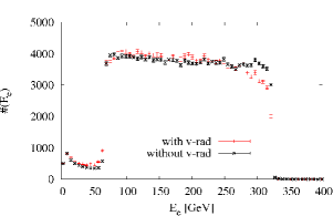
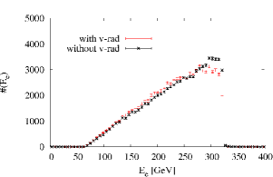
Whether and how well one would actually be able to observe these endpoints will be very model and detector dependant. Regardless of the background or detector sensitivity, we expect that the endpoints of the distribution will have low statistics, given that they correspond to extreme kinematical configurations. Most likely, one will need to rely on data points in the shoulder region to fit the curve and extrapolate the endpoint . These shoulder data points would be the ones most affected by the radiation, so the mass and inferred from them would be significantly different when hidden radiation is included. On the one hand, the curve corresponding to having valley radiation is always softer than the one without, so some mean of the threshold region will give too low an endpoint. On the other hand, if one only tries e.g. a linear fit, the shape of the fall-off in the threshold region would suggest too high an endpoint. A readiness to include a parametric shape for the endpoint region, that takes into account a tuneable radiation contribution, will help ensure a better extraction of the relevant mass parameters.
Notice that the curve corresponding to having valley radiation always lies below the one without, implying that the value of with the radiation would always be higher than the one without. This is a reflection of the two mechanisms we mentioned in the previous section: first, the the valley gluons subtract energy from the , ultimately subtracting it from the s, and second, when they are emitted by the , they change its effective mass, , as one may see in Fig. 4, again subtracting energy from the decay .
Would it be possible to describe the curves with hidden radiation using a model without it, but with different mass parameters and ? Fig. 7 shows the effects of changing the invisible particle mass in model with and without radiation. The ”fingerprint” of the v-radiation is clear: a softening in the shoulder of the distribution which leaves the endpoints fixed. A simple change in the mass parameters of the model without hidden radiation (in this case ) changes the endpoints and leaves the sharp drop of the shoulder unchanged.
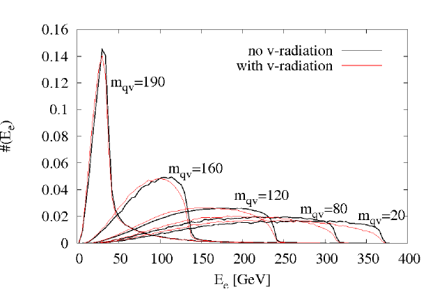
Notice how so long as the mass difference GeV one may always distinguish between any two curves with and without radiation. This of course dependent.
In Fig. 8 instead one can see the dependence of the energy distribution for the visible electrons in each event. Notice how even for a coupling as low as the effects of the v-radiation on the shoulder region are already sizeable.
There are some parameter regions (e.g. when the -to- mass splitting is small) where the shape of the distribution of the hardest leptons is no longer conclusive in distinguishing between a model with and one without valley radiation. In this case one may consider other observables which have an “orthogonal” dependence on the valley parameters. We studied , linearized sphericity and the number of emitted leptons, for example. There is no unique strategy in this case, one must perform a case by case study of the different observables in the different parameter regions to determine which one displays the largest separation between the model with and the model without radiation. As a general rule, we found that three observables were normally sufficient to distinguish the two.
5.2 Collisions not in the center-of-mass frame: MT2
We now consider the effect of initial-state radiation (ISR). This causes unobservable radiation, mainly along the beamline, but also some transverse kicks. Beamstrahlung is highly machine-dependent and thus not included, but is purely longitudinal. The methods we will introduce to handle bremsstrahlung also automatically handle beamstrahlung with little or no degradation of performance, so from now on we will not address the latter specifically.
For our theoretical studies, in order to avoid the clustering of ISR radiation with the leptons coming from the hard interaction, we apply a cut on the . The symmetry of the system now being cylindrical, we also changed the clustering algorithm to the cylindrical fastjet [14].
The major consequence of ISR is that the collision now no longer happens in the CM rest frame, with the information connected to the , the momentum along the beampipe, no longer available. In this case it is convenient to introduce a new variable called Cambridge MT2, see [15].
The MT2 variable was invented precisely to treat events in which the new particles are pair-produced and then each decay into one particle that is directly observable and another particle whose existence may only be inferred from from missing transverse momenta.
This observable is somewhat inspired by the transverse mass used at hadron colliders to measure the mass of the boson in the decay . The neutrino escapes detection, its only trace in the detector being missing momentum. In this case one can construct the variable
| (4) |
Here is defined as , although in this particular case the electron and neutrino masses can be neglected, of course. The variable has the property that
| (5) |
If there is enough statistics to ensure that the kinematic configuration corresponding to the maximum is hit, this gives a measurement of (a lower bound on) the mass. Analogously, one may build a variable called MT2, with the property that its upper bound describes the mass of the communicators, i.e. the particles that were pair-produced.
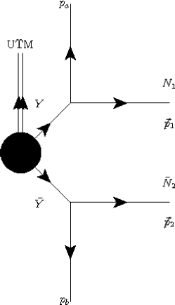
Now consider the process described in Fig. 10. Two particles are pair-produced, then each of them decays into a visible particle ( or in the figure) and one that escapes detection, called . One cannot use the transverse momentum in this case since there are two particles escaping detection, both contributing to the missing transverse momentum . The observable MT2 is defined as
| (6) |
where are all the possible 2-momenta taken away by the s, such that their sum gives the observed missing momenta, .
MT2 coincides with the mass of the communicator , i.e. MT2 has a maximum, when for both communicator decays the visible and the invisible particles are produced at the same rapidity and
| (7) |
For the studies in this article we used a particularly simple version of the MT2 algorithm [20], the source code of which can be downloaded from
http://daneel.phyics.uc.davis.edu/ Cheng:2008hk/mt2-1.01a/test.
A more sophisticated algorithm is described in [23].
The simpler method is based on the use of ”kinematic constraints” [21, 22, 17, 20]
| (8) |
In the case of two invisible and at least two visible particles as in Fig. 10 the two methods actually coincide [20].
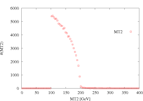
The inputs of the MT2 method are , , , , and . Notice that and may change quite substantially from event to event, since they each correspond to the invariant masses of the clustered visible particles (in this case the lepton and the photons) of each branch. The output of the MT2 method is one single MT2 value per event. Fig. 10 illustrates a typical use of the MT2 variable. If one histograms the MT2 values over a large number of events, the upper edge of this distribution gives a lower limit on the communicator mass .
Whether the event rate in the upper-edge kinematic region defined in eq. (7) is large enough to be able to extract the endpoint MT2, for a given luminosity, depends of course on the interactions. Even more than for the energy variable in the previous section, it is not unlikely that MT2max might have to be extrapolated from points in the shoulder region.
There are many other methods to determine mass relations between the the new particles, [17, 18], just to cite some. Some of these are very closely related to MT2, such as [19]. Some of these require cascade decay chains, or make assumptions about the new particles involved in the decay chain being on shell, or require high luminosity. Where this information is actually available, one should of course make use of it, [24, 25].
The assumptions in this study, though, are that each of the identical decay chains consists of a single two-body decay and that the integrated luminosity, at least for the LHC at 7 TeV study, might be rather low (1 fb-1). These effectively preclude the use of many of the above methods.
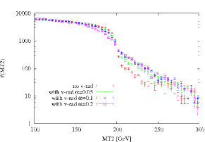
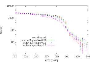
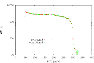
In Fig. 11 one may see the effect of the valley radiation on the MT2 distribution for different values and communicator mass parameters. The interesting region is again represented by the ”shoulder” of the distribution. Notice how the amount of invisible radiation, and thus the effect on MT2max, increases with , analogously to what happens in the energy distributions. The size of these effects may be compared with the effects coming from ISR, in Fig. 12.
The MT2 distribution might present a tail, due to the Breit-Wigner spread that we allow for, see Fig. 13. As one may see, all the MT2 data points which lie above GeV correspond to s which actually have a larger mass than the nominal .
As we already stated above, , the mass of the invisible particle, is an input parameter. MT2max only gives one single relation between and . Depending upon the decay chain topology and the presence or not of upstream transverse momentum (UTM, in the following, may come from ISR or from previous decays), there are different strategies to determine both masses simultaneously: the MT2 “kink” method [19], the invariant mass endpoint [26, 27, 28, 29] or the constrained kinematic method [24], the polynomial intersection method [25], and reconstruction [30, 31, 32], just to cite some possibilities. Most methods, however [26, 27, 28, 29, 24], [25], require longer decay chains (at least two two-body decays) or a special topology, such as 4 on-shell intermediate resonances [24] or 5 or more on-shell intermediate resonances [25].
If each decay chain consists of a single two-body decay, where the visible one may or may not be a composite of visible particles, as described in Fig. 10, one may use the MT2 ”kink method” [19] to fix the value of , i.e. exploit the fact that MT2max as a function of the invisible particle trial mass has a ”kink” for . The authors of [33] point out that in order to have a substantial change in the gradient , there must be substantial event-by-event changes, though. This can be triggered by substantial differences in the , caused by the visible system being a collection of two or more particles, or by a large UTM. Otherwise the kinematics is so constrained that the gradients for and have to be the same, and no kink is possible.
If a sizable UTM is present, one may use the MT2 method [34]. This method uses the fact that , the number of times the is larger than , has a minimum for . The advantage of using this method rather that MT2kink is that may be calculated analytically and measured using the whole data sample, regardless the . This may be shown by using the fact that corresponds to MT2,
| (9) |
the one-dimensional analogue of MT2, where
and where and refer to the projections of the along the direction of the UTM.
We will not discuss further the different methods to extract the two new particle masses, but refer the interested reader to the proceedings from the TeV 2009 [16] conference and to the review [33]. We however wish to make a few remarks about the impact that valley radiation might have on these observables. Consider the MT2 case, for example.
In the presence of valley radiation one needs to consider two sources of deviations. Firstly, the tails coming from the interleaved radiation mechanism, see the MT2 distributions in Fig. 11. Secondly, as discussed in the previous section, in the presence of valley radiation, we expect the mean value of the invisible particle invariant mass to shift from its Breit-Wigner central value towards the communicator mass (or ) value. We will show in subsection 6.2 that the MT2 distribution one obtains may be significantly affected, see Fig. 4 for th LHC case. The should be similarly affected. The number of events having would then change accordingly, as would the minimum point .
We will return on the issue of the the trial mass and the radiation in subsection 6.2. In the following, unless otherwise specified, the analysis will always assume .
6 Effects of radiation at LHC
At LHC the communicators are (mostly) pair-produced by or fusion and decay flavour diagonally into a SM quark and a valley . For our study we assume the s to be spin 1/2 particles, and the s to be scalars. As earlier this choice affects the production cross section, but now both - and -channel exchange are involved, which complicates the pattern. Each radiates both SM s and valley s. These in turn may radiate further s and s, respectively. Once the has decayed, the radiates gluons, while the radiates s. The amount of hidden radiation emitted depends upon the valley coupling constant and on the mass ratio , see Fig. 4. At the LHC the communicator mass reach will be larger than for the ILC, so typically there will be more phase space available for the radiation. Both the valley gluons radiated by the and those radiated by the have an impact on the visible particle distributions. The lighter the particle, the lower the cut-off scale for the radiation however, so it will be the that radiates the most, as before.
When compared with the CLIC case, the LHC scenario presents several complications. Firstly one needs to convolute the production cross section with parton distribution functions. Thus the hard interaction — the production of the pair — no longer happens in or close to the center-of-mass rest frame. In this case it is crucial to consider longitudinally boost invariant observables such as MT2. Secondly, both initial- and final-state QCD radiation are more intense than the QED one is for the ILC case, resulting in a considerably larger upstream transverse momentum and an increased misassignment of radiation. Thirdly, there is an underlying-event activity that gives rise both to a generic low- background and to occasional further hard partons that may be confused with the ones related to the valley process. Fourthly, the partons hadronize into more-or-less well-defined hadronic jets, the reconstruction of which introduces further smearing of the relevant kinematic distributions. And finally, the set of possible background processes is much more varied and challenging to suppress. In our study we will take into account the first four points, but leave the last one to the experimental community, where already a large number of background-suppression techniques have been developed for various scenarios.
6.1 LHC with 7 TeV
The LHC will initially be running at of TeV and it is expected to deliver 1 fb-1 of data in 2010–2011. Under these conditions we need to consider much lower masses for the communicator than for the ultimate energy and luminosity case, in order to have large enough production cross sections, see Table 2.
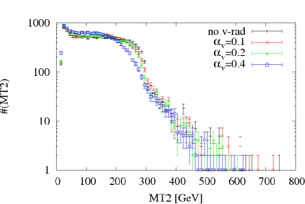
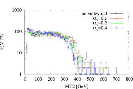
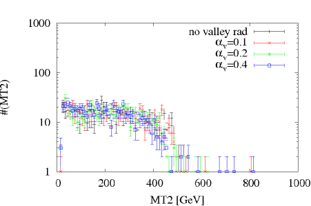
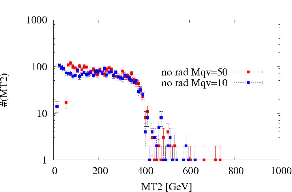
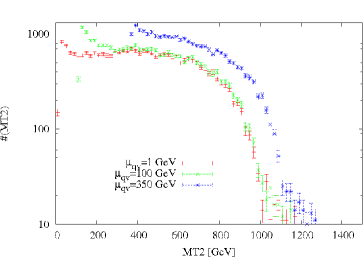
Based on the above discussions, we choose to study the MT2 distribution, and specifically its dependence on the v-radiation and on the value. In Fig. 14 we have plotted the dependence for three different mass values and 500 GeV. The larger the mass difference the more phase space is available for the radiation. The smaller the , the lower the cut-off on the momenta, so the larger the amount of soft radiation. Given the low statistics, the (purely statistical) error bars on the endpoints are rather large, and even in the shoulder of the distribution it is hard to distinguish the curve with an from the curve with no radiation for the 300 GeV mass. In the intermediate case GeV, we need to have a rather strong coupling before the two curves can be separated.
In Fig. 15 we show the MT2 dependence on the invisible mass , where the trial mass is assumed to coincide with . Whether we look at the curves with a valley radiation (valley coupling , left plot in Fig. 15) or at the curves without hidden radiation (right plot in Fig. 15), the data points corresponding to GeV are hardly distinguishable. The independence of the MT2 on the value appears to be a characteristic which the radiation leaves unchanged.
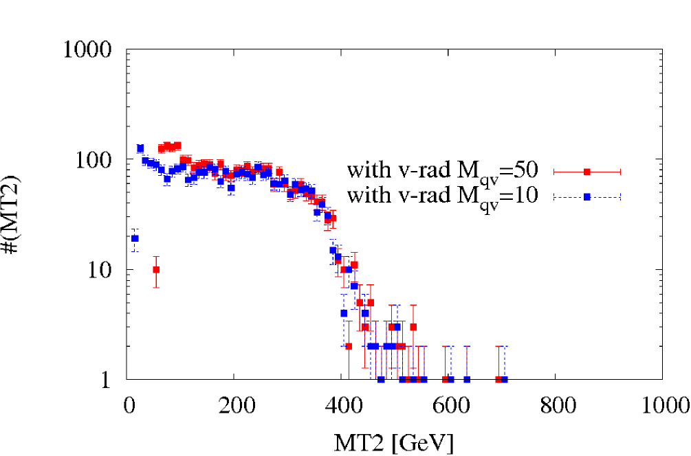
One could argue that the fact that MT2 is hardly dependent on the is due to the mass ratio being fairly large compared to the difference between the two values we considered. Would this argument still hold true when the v-radiation is larger?
For larger values of the one should consider the fact that the MT2 input parameter corresponds to the mass of the as seen by the visible particles. The visible particle momenta, i.e. the momenta of the and the radiated by it, which enter MT2, actually correspond to the invariant mass rather than the nominal mass value .
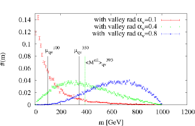
In Fig. 4 we show this invariant mass distribution and how this changes as a function of the coupling constant . As grows emits more and more valley gluons . The invariant mass of the s system then grows, i.e the mean effective mass of the as seen from the SM shifts from the bare GeV towards . The energy which is left for the quark then gets smaller as the as shown by
| (10) |
where for simplicity we have put the .
Were this distribution a very narrow peak around , there would be no difference between the two cases in Fig. 16 so long as , i.e. between a fixed value and an invariant mass distribution. One could speculate that so long as the mean value of the invariant mass the MT2 would basically remain unaffected.
Imagine though having a v-radiation large enough to shift the substantially, , e.g. . One would naïvely think that replacing the with would give a better description of the case with radiation. However Fig. 4 shows that for the invariant mass distribution would also have a large spread around this central value. We will show in the next section that this spread causes further complications. It is precisely the spread in the distribution which constitutes the difference between case a) and case b), and it is this spread which is ultimately responsible for the different behaviour of the MT2 in the two cases.
6.2 LHC with 14 TeV
If we now assume that LHC will collect fb-1 of data at center of mass energy 14 TeV, then one may consider larger communicator masses, , and still deal with a sufficient number of events, see Table 2. If the remains light, the mass ratio can be considerable and consequently the phase space available for radiation can be large. We expect the effects of the radiation to be significant.
In Fig. 17 we show the dependence of the MT2 distribution on the hidden valley coupling constant , assuming we know the mass of the invisible particle so . In this case we are describing the strong coupling regime .
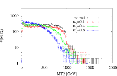
Notice how in this case one can actually separate (at least before any background or detector simulation is taken into account) the curve with and the one without the radiation.
In the above study the assumption is that events are generated with a bare mass and analyzed with the same (or almost the same) trial mass . From the discussion in subsection 5.2, we could conclude that it is not very likely that we would know the mass of the with high precision when valley radiation is present.
In a hidden valley scenario the mass of the is assumed to be much lighter than the mass, so we do not expect the MT2 to be very sensitive to mass differences of the order . Indeed, the authors of [19] and [33] show that the MT2max mass dependence on the trial mass is rather weak so long as , whereas MT2max grows much more rapidly when . The case is exactly what one observes in Fig. 18.
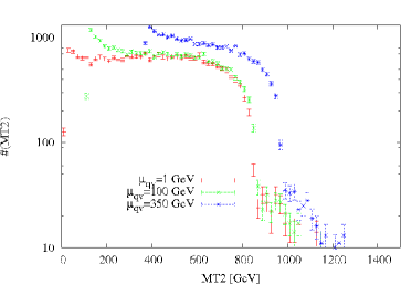
Let us however make the conservative assumption that we only know the order of magnitude of the . Imagine trying to distinguish between the two models we described in Fig. 16, a) the model with no radiation and b) the model with the radiation, when . To be more concrete, assume a) has a fixed value mass GeV and b) has an invisible particle mass GeV and . We choose the value so that .
In Fig. 18, left side, we see the MT2 distribution for model a) for the case TeV. As one may observe, this is a function of the trial mass , the best profile being the one with . For , even for substantial changes in the MT2max does not change much. This essentially confirms what was reported by [19, 33].
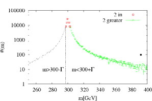
On the right side of Fig. 18 one may see the same distributions for the model with radiation. Contrary to what one would expect from the naïve arguments given in the previous subsection, we see that choosing does not give the best description of the system. The MT2 curve overshoots the value by a good 10%. As anticipated in the previous subsection, this is due to the invariant mass distribution spread. Looking at Fig. 20, one may see that the invariant mass distribution has a wide spread, so event by event there could be large variations in the . If one chooses a to analyze the set of events, for example the GeV chosen in Figure 18, most of the events will have a ”real” mass, the invariant mass , larger than the trial mass . Since MT2 MT2 when , these points do not contribute to increase the MT2max value much, and the distribution will resemble rather closely the one obtains for GeV, apart from the softening in the shoulder. This is precisely what happens in the GeV curves in Fig. 18.
When one takes a instead, e.g. GeV (which according to the naïve arguments of the last subsection should have been the best of the three choices), more and more events have a ”real” invisible particle mass . In Fig. 20 these are the points to the left of the GeV line. These events will, if there is enough statistics, give MT2MT2, the real value. This is what happens to the curve for GeV.
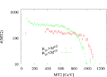
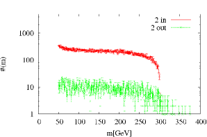
To prove this point, we separately plot the MT2 distributions for the events with and the ones with . As Fig. 20 shows, for the former set MT2.
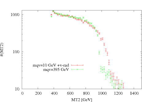
This said, we may return to the issue of distinguishing between the two models a) and b). As one may see in Figure 21, the two curves corresponding to the two models have very different shapes, the one with no radiation being the sharper one. Notice however that now the curve with radiation lies above the one without. This is not in contradiction with what we have shown in the previous sections.
Summarizing, in the not-so-strong coupling regime , when the invariant mass distribution is strongly peaked in , one may333At least before background and detector analysis. distinguish two models with the same values for and , one with v-radiation and one without. The curve corresponding to the no hidden radiation model will have a steeper drop in the shoulder region.
For larger couplings, , one should note that two MT2 distributions with the same endpoints may correspond to different values in the two cases, depending on whether the majority of the events have an invariant mass which is greater or smaller than the trial mass. A very conservative approach to solving this problem could simply be to assume GeV or in any case .
7 Conclusions
We have here addressed the issue of detecting and identifying hidden radiation through its influence on SM parton showers, and in general through its impact on visible particle kinematic distributions. We have done so in the context of Hidden Valley models, which we find are well suited to display the effects, but the specific models studied should be viewed only as representatives of a broad range of possible models with new symmetries. Thus, while we focus on the phenomenology of a fairly generic toy model, we also provide tools in Pythia 8 to simulate the effects of hidden radiation in various other hidden valley scenarios, e.g. different gauge groups, particle contents, and gauge and decay couplings. The novel feature in these tools is the interleaved SM and valley parton shower, i.e. the competition between visible and hidden radiation.
Our preliminary study of the phenomenology of the toy model at and at LHC colliders shows the following.
At an 800 GeV ILC collider we could expect to observe hidden radiation for valley gauge couplings as small as , so long as the mass of the communicator is smaller than 300 GeV and .
For the LHC phenomenology we need to distinguish between the first two year running with TeV and fb-1 and later years with full design energy TeV and fb-1. Whether one could observe hidden radiation or not depends strongly on the communicator mass, which determines the amount of statistics. The main signal of the hidden radiation — at least in our studies — is the softening of the shoulder of the MT2 distribution. In the lower-energy case, for communicator masses around 500 GeV or higher, the statistics is so poor that one cannot expect to distinguish even a very strong coupling . For two models with and without hidden radiation, with equal masses in the [300, 400] GeV range and equal GeV, one would need a valley coupling of the order or larger to induce large enough effects on the MT2 distribution to distinguish between the two. In the higher-energy case, for order TeV communicator masses and smaller than 100 GeV, the MT2 distributions show sizable changes already for .
We have also studied how the MT2 distribution depends upon the , the invariant mass , and the trial mass . In the case of a Hidden Valley scenario, is always assumed to be . Taking a trial mass as an input parameter for the MT2 is thus a natural choice. When the mass is larger though, e.g. , the issue of the trial mass is no longer so trivial. The can be a broad distribution when radiation is present. Especially in the strong interaction case, , is strongly shifted towards . This means that when one chooses a trial mass , roughly half of the events will have , causing the MT2max to overshoot the real value. In this case the new masses thus have to be extracted from a combined fit, in which both masses and couplings enter as unknowns.
Further studies of the background and detector simulations should follow, both for the kind of scenarios we have explored here and for other possible ones. This preliminary study, however, shows unequivocably that parton showers are a key tool in determining the presence of new hidden gauge groups and in the exploration of the hidden sector gauge group dynamics.
Acknowledgments.
We would like to thank Peter Skands for suggesting this study and for the profitable exchanges we had throughout the whole project. We also acknowledge helpful discussions with Matt Strassler.References
- [1] M. J. Strassler and K. M. Zurek, “Echoes of a hidden valley at hadron colliders,” Phys. Lett. B 651, 374 (2007) [arXiv:hep-ph/0604261].
- [2] H. Georgi, “Unparticle Physics” Phys. Rev. Lett. 98, 221601 (2007) [arXiv:hep-ph/0703260].
- [3] R. Blumenhagen, M. Cvetic, P. Langacker and G. Shiu, “Toward realistic intersecting D-brane models,” Ann. Rev. Nucl. Part. Sci. 55, 71 (2005) [arXiv:hep-th/0502005].
- [4] Z. Chacko, H. S. Goh and R. Harnik, “The twin Higgs: Natural electroweak breaking from mirror symmetry,” Phys. Rev. Lett. 96 (2006) 231802 [arXiv:hep-ph/0506256].
- [5] M. J. Strassler, “Possible effects of a hidden valley on supersymmetric phenomenology,” arXiv:hep-ph/0607160.
- [6] K. M. Zurek, “Multi-Component Dark Matter,” Phys. Rev. D 79 (2009) 115002 [arXiv:0811.4429 [hep-ph]].
- [7] M. J. Strassler, “Why Unparticle Models with Mass Gaps are Examples of Hidden Valleys,” arXiv:0801.0629 [hep-ph].
- [8] J. Kang and M. A. Luty, “Macroscopic Strings and ’Quirks’ at Colliders,” JHEP 0911, 065 (2009) [arXiv:0805.4642 [hep-ph]].
- [9] T. Sjöstrand, S. Mrenna and P. Z. Skands, “A Brief Introduction to PYTHIA 8.1,” Comput. Phys. Commun. 178, 852 (2008) [arXiv:0710.3820 [hep-ph]].
- [10] C. Amsler et al. [Particle Data Group], Phys. Lett. B 667 (2008) 1.
- [11] V. M. Abazov et al. [D0 Collaboration], “Search for scalar leptoquarks in the acoplanar jet topology in collisions at = 1.96-TeV,” Phys. Lett. B 640 (2006) 230 [arXiv:hep-ex/0607009].
- [12] V. M. Abazov et al. [D0 Collaboration], Phys. Rev. Lett. 99 (2007) 061801 [arXiv:0705.0812 [hep-ex]].
- [13] E. Norrbin and T. Sjöstrand, “QCD radiation off heavy particles,” Nucl. Phys. B 603, 297 (2001) [arXiv:hep-ph/0010012].
- [14] M. Cacciari and G. P. Salam, “Dispelling the myth for the jet-finder,” Phys. Lett. B 641, 57 (2006) [arXiv:hep-ph/0512210].
- [15] C. G. Lester and D. J. Summers, “Measuring masses of semiinvisibly decaying particles pair produced at hadron colliders,” Phys. Lett. B 463, 99 (1999) [arXiv:hep-ph/9906349].
- [16] G. Brooijmans et al., “New Physics at the LHC. A Les Houches Report: Physics at TeV Colliders 2009 - New Physics Working Group,” arXiv:1005.1229 [hep-ph].
- [17] I. Hinchliffe, F. E. Paige, M. D. Shapiro, J. Soderqvist and W. Yao, “Precision SUSY measurements at LHC,” Phys. Rev. D 55, 5520 (1997) [arXiv:hep-ph/9610544].
- [18] D. R. Tovey, “Measuring the SUSY mass scale at the LHC,” Phys. Lett. B 498, 1 (2001) [arXiv:hep-ph/0006276].
- [19] W. S. Cho, K. Choi, Y. G. Kim and C. B. Park, “Gluino Stransverse Mass,” Phys. Rev. Lett. 100, 171801 (2008) [arXiv:0709.0288 [hep-ph]].
- [20] H. C. Cheng and Z. Han, “Minimal Kinematic Constraints and MT2,” JHEP 0812, 063 (2008) [arXiv:0810.5178 [hep-ph]].
- [21] H. Bachacou, I. Hinchliffe and F. E. Paige, “Measurements of masses in SUGRA models at CERN LHC,” Phys. Rev. D 62, 015009 (2000) [arXiv:hep-ph/9907518].
- [22] B. C. Allanach, C. G. Lester, M. A. Parker and B. R. Webber, “Measuring sparticle masses in non-universal string inspired models at the LHC,” JHEP 0009, 004 (2000) [arXiv:hep-ph/0007009].
- [23] C.G. Lester “mT2 homepage” [http://www.hep.phy.cam.ac.uk/ lester/mt2/index.html].
- [24] H. C. Cheng, J. F. Gunion, Z. Han, G. Marandella and B. McElrath, “Mass Determination in SUSY-like Events with Missing Energy,” JHEP 0712, 076 (2007) [arXiv:0707.0030 [hep-ph]].
- [25] H. C. Cheng, D. Engelhardt, J. F. Gunion, Z. Han and B. McElrath, “Accurate Mass Determinations in Decay Chains with Missing Energy,” Phys. Rev. Lett. 100, 252001 (2008) [arXiv:0802.4290 [hep-ph]].
- [26] B. K. Gjelsten, D. J. . Miller and P. Osland, “Measurement of SUSY masses via cascade decays for SPS 1a,” JHEP 0412, 003 (2004) [arXiv:hep-ph/0410303].
- [27] D. Costanzo and D. R. Tovey, “Supersymmetric particle mass measurement with invariant mass correlations,” JHEP 0904, 084 (2009) [arXiv:0902.2331 [hep-ph]].
- [28] M. Burns, K. T. Matchev and M. Park, “Using kinematic boundary lines for particle mass measurements and disambiguation in SUSY-like events with missing energy,” JHEP 0905, 094 (2009) [arXiv:0903.4371 [hep-ph]].
- [29] K. T. Matchev, F. Moortgat, L. Pape and M. Park, “Precise reconstruction of sparticle masses without ambiguities,” JHEP 0908, 104 (2009) [arXiv:0906.2417 [hep-ph]].
- [30] K. Kawagoe, M. M. Nojiri and G. Polesello, “A new SUSY mass reconstruction method at the CERN LHC,” Phys. Rev. D 71 (2005) 035008 [arXiv:hep-ph/0410160].
- [31] M. M. Nojiri, G. Polesello and D. R. Tovey, “A hybrid method for determining SUSY particle masses at the LHC with fully identified cascade decays,” JHEP 0805, 014 (2008) [arXiv:0712.2718 [hep-ph]].
- [32] B. Webber, “Mass determination in sequential particle decay chains,” JHEP 0909, 124 (2009) [arXiv:0907.5307 [hep-ph]].
- [33] A. J. Barr and C. G. Lester, “A Review of the Mass Measurement Techniques proposed for the Large Hadron Collider,” arXiv:1004.2732 [hep-ph].
- [34] P. Konar, K. Kong, K. T. Matchev and M. Park, “Superpartner mass measurements with 1D decomposed MT2,” [arXiv:0910.3679 [hep-ph]].