Glassy aspects of melting dynamics
On melting dynamics and the glass transition, Part I

Abstract

The following properties are in the present literature associated with the behaviour of super-cooled glass-forming liquids: faster than exponential growth of the relaxation time, dynamical heterogeneities, growing point-to-set correlation length, crossover from mean field behaviour to activated dynamics. In this paper we argue that these properties are also present in a much simpler situation, namely the melting of the bulk of an ordered phase beyond a first order phase transition point. This is a promising path towards a better theoretical, numerical and experimental understanding of the above phenomena and of the physics of super-cooled liquids. We discuss in detail the analogies and the differences between the glass and the bulk melting transitions.

Almost any liquid becomes a glass when cooled fast enough GLASS-GEN:1 ; GLASS-GEN:2 ; ANGELL . Many different scenarios and theories have been proposed over the time to describe the nature of glasses. Yet, it is still not known what is the fundamental principle behind the experimentally observed abrupt change in the relaxation time of super-cooled liquids. Is there an underlying critical phenomenon behind the glass transition or not? Is the glass transition a thermodynamic or purely dynamic notion? What is the correct theory of super-cooled liquids? These questions remain unanswered and widely discussed.

It is the experimental and numerical observations on super-cooled liquids that remind us of thermodynamic phase transitions. The most remarkable experimental facts about the transition from liquids to glasses are indeed: (a) The extremely fast rise of the relaxation time $\tau$, that increases easily by several orders of magnitude as the temperature is decreased by a few percent. It is well approximated by the Vogel-Fulcher-Talman law $\tau\propto\exp{[A/{\left(T-T_{VFT}\right)}]}$ VogelFulcher . (b) The extrapolated temperature $T_{\rm VFT}$ is found to be very close to the Kauzmann temperature $T_{K}$ where the extrapolated entropy of the supercooled liquid becomes smaller than that of the crystal Kauzmann . (c) The Adam-Gibbs relation $\tau\propto\exp{[C/\Delta S(T)]}$ AdamGibbs , where $\Delta S(T)$ is the difference between the two entropies, is observed with a good accuracy.

It has been suggested that this quasi-universal behaviour should be related to the existence of a length scale growing as the glass transition is approached, and the hunt for such a length has been a central theme in the field in the last decade. A purely dynamical quantity, proposed originally in the context of mean-field spin glasses Silvio , uses a four-point density correlator in both time and space, and has led to the notion of dynamical heterogeneities and to the so-called dynamical susceptibility (usually refereed to as $\chi_{4}$). Indeed, the growing of dynamical heterogeneities has been observed in glass formers DynBB ; DynHS . By contrast, other groups have considered the possibility of a static (thermodynamic) growing length scale and proposed the point-to-set correlation, that is the correlation of a sub-system with its frozen boundaries BiroliBouchaud ; DynamicBethe ; PointToSet . Recent numerical and experimental works confirmed that indeed there seems to be such a growing thermodynamic length scale in supercooled liquids PTS-Exp-Num .

One of the standard routes to the above phenomenology goes through the Random First Order Theory (RFOT) KT ; KW1 ; KW2 ; KTW ; GlassMezardParisi according to which a good starting point of the glass phenomenology are mean-field spin glasses, and in particular the $p$-spin glass model REM ; P-SPIN ; XORSAT ; MPV . Mean-field spin glasses have an interesting phenomenology: they behave like a liquid/paramagnet at large temperature, and when cooled down the equilibration time diverges as a power law at a temperature $T_{\rm MCT}$ and the relaxation process is described by the Mode-Coupling Theory (MCT) MCT ; MCT2 ; BiroliBouchaudMCT ; Kurchan ; DYNAMIC ; AndreaSaddle . The true thermodynamic glass transition, however, arises at $T_{K}<T_{\rm MCT}$ in these models. According to RFOT, the correct theory of the glass transition is the finite dimensional counterpart of this behaviour. A phenomenology called the the mosaic picture AdamGibbs ; KW1 ; KW2 ; KTW ; BiroliBouchaud is used in order to explain that in structural glasses the relaxation time diverges only at $T_{K}$. This crossover from the power-law divergence at $T_{\rm MCT}$ (in the mean-field) to the super-exponential divergence at $T_{K}$ (in finite dimension) is at the root of the RFOT theory. The validity of this picture is still, however, disputed (see for instance Langer ; BiroliBouchaud09 and references therein).

In this work, we argue that the above phenomena, usually associated in the present literature with the dynamics of supercooled liquids close to the glass transition, also appear in a much simpler problem – the bulk melting process of the fully ordered phase above an ordinary first order phase transition. All the following ingredients arise: the crossover from a power-law divergence of the relaxation time to an activated dynamics and a Vogel-Fulcher-Talman-like divergence; the presence of a growing length scale associated with point-to-set correlations; the divergence of the dynamical susceptibility and the presence of dynamical heterogeneities; the presence of a plateau in the dynamical correlation function with increasing life-time as the transition is approached.

Analogies between the glass transition and the first order phase transitions are often evoked – as testified by the very name of the random first order theory. We argue that the extend to which these analogies are valid and useful is larger than previously anticipated. The existence of this correspondance calls for more detailed theoretical, numerical and experimental investigations in systems with a first order phase transition. It offers a simpler way to understand some of the aspects and phenomenology of glassy dynamics, and inversly provides new ways to look at the bulk melting problem as well.

In a subsequent paper US-PART-II , we shall go beyond a simple analogy and show that in some systems there is an exact mapping between the equilibrium glassy dynamics and the melting of ordered phase. This is true in particular in the mean field $p$-spin models REM ; P-SPIN ; XORSAT , and also on the Nishimori line Nishimori-Original ; Nishimori in finite dimensional systems.

This paper is organized as follows: In the first section, we briefly introduce the melting problem in systems with a first order phase transition, and stress the differences between surface melting and bulk melting. In the second section, we review the properties of bulk melting above a first order phase transitions on the mean-field level. As an example we use the exactly solvable $p$-spin ferromagnet on a fully connected lattice, that undergoes a first order ferromagnetic phase transition. In the third section, we move to the finite dimensional case, and discuss briefly the nucleation and growth arguments to predict properties of melting in finite-dimensional systems. In the fourth section, we simulate numerically the Potts model on a two dimensional lattice to show that indeed most of the phenomenology discussed in the glass transition in finite dimensional systems arises generically also during the melting of the ordered phase. Section V explains two crucial differences between dynamics of super-cooled liquids close to the glass transition and melting in a generic system with a first order phase transition. In the subsequent paper US-PART-II we then study systems with a first order transition where these differences disappear. We finally review our results and discuss some criticisms of the RFOT scenario in the light of our findings.

I Bulk melting

In this section we specify what we mean by melting process above a first order phase transition, and in particular we emphasize that we deal here with bulk melting SurfaceMelting_R1 , instead of the much studied —and arguably more practically important— surface melting process.

Consider a system with a first order phase transition, for instance the solid-liquid transition in crystalline structures or in three-dimensional hard spheres HardSphere , or any given ferromagnetic spin system with a first order transition such as the Ising model in field or the Potts model in temperature Wu . Start in the fully ordered state (the crystal for solids, the perfect packing for hard spheres, or the completely magnetized state in the spin models) and suddenly change the pressure/temperature/field in order to put the system in the liquid/paramagnetic/less ordered phase. The system will melt. How long does this melting process take, and what are its properties? How does a solid turn into a liquid?

The occurrence of a discontinuous transition suggests that melting of crystalline or solid matter in nature is a first order phase change that requires a finite latent heat, and a nucleation mechanism. This is indeed the case provided some precautions are taken. Consider for instances solids, unlike super-cooling of liquids, super-heating of crystalline solids is observed to be extremely difficult if not impossible SurfaceMelting_R1 ; SurfaceMelting_R2 ; SurfaceMelting_R3 in most experiments. This peculiarity is due to the fact that melting of a crystal kept at a homogeneous temperature always begins on its free surface. Surface melting is indeed the dominant mechanism for melting of solids in nature, as it is a much faster process than the bulk melting. It was, however, realized that by suppressing surface melting Superheating super-heating to temperatures well above the equilibrium melting point could be achieved. In this case, one recovers the nucleation phenomenology of first order phase transitions, and this is the kind of melting processes that, as we will show, displays many analogies with glassy dynamics. Such bulk melting problems and the study of the super-heated solids have received a boost of experimental and theoretical studies recently Superheating ; SuperANDHetero .

Here, we shall work with very simple models, far from realistic atomic or sphere systems. Our motivation stems from the fact that we expect properties of bulk melting to be universal and to be qualitatively similar in solids, magnetic systems, hard spheres or polymers with a first order transition. Following the classical mapping between spin systems and lattice gas LatticeGas , we will concentrate on the first order transition in Ising and Potts spin models. Since these models are more easily amenable to analytic studies and simulations, this will allow us to discuss universal behaviour, such as spinodal and nucleation mechanisms. Moreover, in theoretical considerations surface melting can be suppressed by simply using fixed or periodic boundary conditions. Finally, many activities in studies of the glass transition have been devoted to spin models, this is hence a natural setting for discussing the analogies between glassy and melting dynamics.

II Melting in mean-field systems

In this section, we start by discussing the bulk melting transition at the mean-field level using a simple solvable model. An elementary example of a mean-field system with a first order phase transition is the fully-connected ferromagnetic $p$-spin Ising model, for $p=3$

$${\cal H}=-J\sum_{ijk}S_{i}S_{j}S_{k},$$ (1)

where the sum is over all $N^{3}$ values of indices $i,j,k$. This is a simple generalization of the Curie-Weiss model.

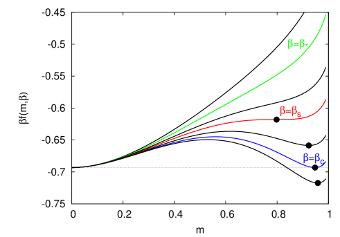
Figure 1: (color online): Gibbs free energy $f(m,\beta)$ as a function of the magnetization $m$ for different temperatures $\beta$ for the ferromagnetic fully-connected 3-spin model. The figure includes the free energy at the critical temperature $\beta_{c}=0.67209$ (blue), at the spinodal temperature $\beta_{s}=0.57217$ (red), and at the temperature where the free energy starts to be a convex function of the magnetization $\beta_{*}=0.435$ (green). This illustrates the generic behaviour of the free energy in a mean-field system with a first order phase transition.

II.1 The static behaviour

Just like the Curie-Weiss model, the ferromagnetic $p$-spin model is exactly solvable on a fully connected lattice (which is a very crude mean-field approximation to the finite dimensional case). To ensure extensivity of the thermodynamic potentials we take $J=1/N^{p-1}$. The Gibbs free energy as a function of magnetization $m$ and inverse temperature $\beta$ reads (see the appendix):

$$\beta f(m,\beta)=-\beta m^{p}-\log{[2\cosh{\,\text{atanh}{(m)}}]}+{m\,\text{atanh}{(m)}}$$ (2)

while the self-consistent equation for magnetization reads

$$m=\tanh{\left(\beta pm^{p-1}\right)}\,.$$ (3)

As illustrated in Fig. 1, for $p=3$, this yields a first order phase transition at $\beta_{c}=0.67209$. The low temperature ferromagnetic phase is, however, locally stable up to the spinodal point at $\beta_{s}=0.57217$. The Gibbs free energy $f(m,\beta)$ starts to be a convex function of magnetization above temperature corresponding to $\beta_{*}=0.435$.

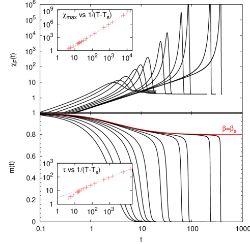
Figure 2: (color online) The melting process starting from the completely magnetized $m(0)=1$ state for different temperatures in the fully connected $3$-spin ferromagnet. Bottom: The time evolution of the magnetization $m(t)$, from left to right, $\beta=0.35$, $0.4$, $0.45$, $0.5$, $0.52$, $0.54$, $0.56$, $0.565$, $0.57$, $0.571$, $0.572$, $0.5721$ and the spinodal temperature (in red) $\beta_{s}=0.57217$. $m(t)$ shows a two-steps relaxation when approaching the spinodal point (that starts to be observable at roughly $\beta_{*}$). The time needed for the system to melt diverges according to eq. (5) (see inset). Top: The dynamical ferromagnetic susceptibility eq. (7) for the same set of temperatures. It has a maximum around $\tau$ and converges at large times to the static value $\chi_{F}=\beta$. The peak of the susceptibility diverges when approaching the spinodal point as eq. (8) (see inset), indicating the growth of a correlated volume.

II.2 The dynamical behaviour

Consider the following Glauber dynamics: At each interval of time $1/N$, we pick up one spin, and set it $+1$ with probability $p_{+}=(1+\tanh{\beta h})/2$, and $-1$ with probability $p_{-}=(1-\tanh{\beta h})/2$, where $h=pm^{p-1}$ is the local field on the spin. This dynamics is also exactly solvable for the fully connected ferromagnetic $p$-spin model (see again the appendix for derivations). The average (over realizations) of the magnetization $\langle m(t)\rangle$ evolves in time according to the following differential equation

$$\frac{{\rm d}\langle m(t)\rangle}{{\rm d}t}=-\langle m(t)\rangle+\tanh{[\beta p\langle m(t)\rangle^{p-1}]}\,.$$ (4)

Fig. 2 shows how the magnetization evolves in time if the system is initialized in the ferromagnetic configuration $m(t=0)=1$ for different temperatures. As the spinodal temperature of the ferromagnetic phase $\beta_{s}$ is approached from above, we observe a two-steps relaxation. The magnetization of the flat region is roughly the magnetization of the appearing metastable state and its length defines the relaxation time. This relaxation time diverges as a power law

$$\tau\propto\left(1-\frac{\beta}{\beta}_{s}\right)^{-\frac{1}{2}}\,.$$ (5)

The flattening of the relaxation process starts roughly at the temperature $\beta_{*}$. The growing plateau in the decay of the order parameter and the power-law divergence of the relaxation time are classical features of a melting process above a mean-field first order transition Binder73 ; ReviewBinder .

II.3 Static and dynamic diverging length scales

Coming back to the discussion in the introduction, one may ask if there is a growing length, or volume, associated with the divergence of this relaxation time. The naive answer is no: The magnetic susceptibility that diverges at a second order phase transition stays indeed finite in systems with a first order phase transition when the ferromagnetic spinodal temperature $T_{s}$ or the critical temperature $T_{c}$ is approached from above. This answer is, however, wrong. Consider the following (time-dependent) correlation function, averaged over many realizations of the melting dynamics

$$C_{ij}(t)=\langle S_{i}(t)S_{j}(t)\rangle-\langle S_{i}(t)\rangle\langle S_{j}(t)\rangle\,.$$ (6)

It is natural to ask how many spins have correlated moves at a given time $t$. An estimates of this is given by integrating this function over the whole system

$$\chi_{F}(t)=\frac{\beta}{N}\sum_{ij}C_{ij}(t)=N\beta\left[\langle m^{2}(t)\rangle-\langle m(t)\rangle^{2}\right]\,.$$ (7)

One recognizes that, for large time, this is nothing but the equilibrium magnetic susceptibility (we have used the multiplication by $\beta$ in order to be consistent with the usual definition of the magnetic susceptibility), and we shall thus call this quantity the dynamic magnetic susceptibility. Certainly the equilibrium magnetic susceptibility is finite in a system with a first order transition when the ferromagnetic spinodal temperature $T_{s}$ is approached from above. Let us look, however, to the finite time behaviour of $\chi_{F}(t)$, it follows a differential equation derived in the appendix. The solution for different temperatures is plotted in Fig. 2.

We see that $\chi_{F}(t,\beta)$ increases with time, reaches a maximum roughly at the relaxation time $t=\tau(\beta)$, and then decays to reach its equilibrium value (which is nothing else than the Curie law for a paramagnet $\chi_{F}=\beta$). The maximum value of $\chi_{F}(\tau,\beta)$ grows, however, very fast as the spinodal point $\beta_{s}$ is approached. The number of spins that are correlated in the melting process is in this system maximum roughly at the relaxation time $t=\tau(\beta)$, and thus diverges at the spinodal point as

$$\chi_{F}(\tau,\beta)\propto\left(1-\frac{\beta}{\beta}_{s}\right)^{-\frac{5}{2}}\,.$$ (8)

This defines the dynamic length (or volume) that diverges at the spinodal in the melting problem. The origin of the critical exponent $5/2$ is elucidated in a recent work IwataSasa10 .

Is there also static volume/length diverging at $\beta_{s}$? Again, the answer is positive. In order to see it, we consider the system with boundary conditions fixed to positive magnetization. In the paramagnetic phase above the spinodal temperature, fixing the boundaries in this way does not influence the equilibrium bulk properties. But how far should the boundaries be to find back the zero magnetization phase? This is a well defined point-to-set correlation length. In a fully connected model it is, however, rather tricky to define boundary conditions. Let us thus consider the model on a tree of fixed finite degree. The model can then be solved with the Bethe-Peierls method (see the appendix). In the large degree limit the model on tree becomes equivalent to the fully connected one, and the magnetization at distance $l$ from the boundaries follows the recursion

$$m_{l+1}=\tanh{\left(\beta pm_{l}^{p-1}\right)}\,.$$ (9)

In Fig. 3 we show how the magnetization evolves with distance from the boundaries. One observes that the distances one has to go in order to recover the zero magnetization diverges when approaching the spinodal point. Actually, since eq. (9) is simply the discrete version of eq. (4), this length diverges as

$$\ell\propto\left(1-\frac{\beta}{\beta}_{s}\right)^{-\frac{1}{2}}\,.$$ (10)

The length $\ell$ we have just defined is in fact well know in the theory of wetting problems BOOKWETTING , where indeed a divergence is expected. Let us point out that the very same diverging length on a tree can be defined in another equivalent way: One takes a finite tree of depth $\xi$ and computes how large $\xi$ needs to be such that the magnetization in the center (or the total magnetization) is bellow a given threshold. On a tree the two definitions are equivalent and the length $\ell$ is equal to the length $\xi$ as the two processes are described by the very same equation. However, the two definitions differ in finite dimensional systems and we will see that it is the second length $\xi$ that is associated to the point-to-set correlation length in finite dimension (while the first one $\ell$ is the finite dimensional wetting length).

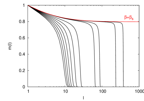
Figure 3: (color online) The magnetization $m_{l}$ at distance $l$ from boundaries fixed to positive magnetization in the paramagnetic phase of the mean-field ferromagnet. From left to right, we show $\beta=0.5,0.51,0.52,0.53,0.54,0.55,0.56,0.57,0.571,0.572,0.5721$ and (in red) $\beta_{s}=0.57217$. The distance one has to go from the boundaries in order to recover the equilibrium magnetization diverges as eq. (10) as the spinodal is approached.

Using the fully connected ferromagnet, we have here described the basic features of the melting process in a mean-field setting. The time $\tau$ needed to decorrelate diverges as the temperature approaches the spinodal point. This translates into a growing plateau in the decay of the order parameter. The divergence of a time scale is accompanied by at least two diverging length scales: the dynamical one, that shows how many spins are correlated in the melting process at the relaxation time scale $\tau$, and a static one, that corresponds to the way the system decorrelates with ordered boundary conditions.

The learned reader will recognize that these two lengths are nothing but the dynamical four-point susceptibility and the point-to-set correlation in disguise. This is the message we want to convey: these length scales defined initially in the mean field theory of the glass transition do also diverge in the simpler situation of the melting of the ordered phase above a first order transition.

At this point, a word of caution should be made: In order to observe these diverging length and time scales when lowering the temperature down to the ferromagnetic spinodal $T_{s}$, it is necessary to start from the ordered phase and to consider its melting towards the high temperature phase. If one instead starts from the equilibrium liquid/paramagnet state, then the phenomenology is much less interesting: the equilibrium relaxation time in the paramagnetic phase does not show any particular interesting feature, apart from increasing when approaching the eventual low temperature paramagnetic spinodal point beyond which the system orders (crystallizes). Of course, if this ordering is avoided a true glass transition could be observed at yet lower temperatures, but this is a different phenomena from the one described above.

III Basics of nucleation theory

In this section, we discuss what happens in finite dimensional systems and recall briefly the classical nucleation theory in order to explain that all the diverging time and length scales discussed above should diverge at the critical point in finite dimensional systems (and not anymore at the spinodal – which is no longer thermodynamically well defined). In the next section, we will illustrate these properties for the two-dimensional Potts ferromagnet.

In finite dimensional systems the free energy density is always a convex function of the magnetization, hence the life-time of any metastable state is always finite. Physically, this is due to the nucleation of the equilibrium phase that is absent in mean-field geometries. Metastability hence becomes a purely dynamical notion and for this very reason giving a proper theoretical definition of a metastable state in finite dimension can be tricky LangerOlder ; CavagnaReview .

Nucleation theory, introduced originally by Gibbs Gibbs , describes the way metastable states decay beyond a first order critical point. The metastable phase has higher free energy, hence it must decay by nucleation of droplets of the stable (lower free energy) phase. Nucleation results from a competition between the bulk free energy difference and the surface tension between the two phases. When a system is in a metastable phase the free-energy cost $\Delta F(\ell)$ of a droplet of size $\ell$ is given by

$$\Delta F(\ell)=-V_{d}\ell^{d}(\delta f)+S_{d}\ell^{d-1}\Gamma\,,$$ (11)

where $V_{d}$ and $S_{d}$ are the volume and surface factors related to the shape of the droplet in dimension $d$, $\delta f$ is the free-energy difference between the two different phases, and $\Gamma$ is the surface tension. The free energy cost is maximum at size

$$\ell_{\rm max}=\frac{(d-1)S_{d}}{dV_{d}}\frac{\Gamma}{\delta f}\,.$$ (12)

Droplets smaller than $\ell_{\rm max}$ have the tendency to shrink, while those larger than $\ell_{\rm max}$ will expand fast (the later process is often described by the Kolmogorov-Johnson-Mehl-Avrami theory Avrami ). In order to relax to equilibrium, thermal fluctuations must cross the free energetic barrier $\Delta F(\ell_{\rm max})$. This nucleation time is often estimated by the Arrhenius formula

$$\tau_{\rm nucl}\approx\exp[\beta\Delta F(\ell_{\rm max})]\approx\exp\left[\frac{A_{d}\beta\Gamma^{d}}{(\delta f)^{d-1}}\right]\,,$$ (13)

where $A_{d}$ is a dimension dependent constant. The first order melting point is defined by $\delta f=0$ and therefore both the nucleation time (13) and the nucleus size (12) diverge at the first-order critical point.

When a critical droplet is formed, it will grow and invade the system. The relaxation process thus depends on both the nucleation time and on the growth of the nucleus. Moreover relaxation can follow from the appearance of many droplets in the system: Indeed the nucleation time $\tau_{\rm nucl}$ gives the average time needed to nucleate a critical droplet at a given place in the system. If, however, the system is much larger than the critical nucleus size (a condition that becomes harder and harder to fulfill as we approach the first-order transition point), the relaxation process will not be done via the growth of a single droplet but instead will result from the nucleation of many droplets that will simultaneously grow and invade the system. Whether the first or the second scenario is happening depends on whether the system size is much larger than the critical nucleus size. In both case, however, the growth time has to be added to the nucleation time to obtain the total relaxation time needed to exit from the metastable state.

Consider a large system, much larger than the size of a critical nuclei. Given the probability to nucleate a critical droplet by a unit of volume and time is proportional to $\rho\propto e^{-\beta\Delta F(l_{\rm max})}\propto 1/\tau_{\rm nucl}$, in a very large system there should therefore be roughly one droplet per volume $\tau_{\rm nucl}$ after a finite time. In most (non disordered) systems, and for most dynamics, the droplet radius is expected to grow as a power law $\ell(t)\propto t^{1/z}$ with time. Therefore, after a time of order $\tau_{\rm nucl}^{z/d}$ droplets will start to touch each other and the portion of the system in the new phase will percolate. This predicts that the relaxation time is $\tau_{relax}\propto\exp\left[\frac{z}{d}\frac{A_{d}\beta\Gamma^{d}}{(\delta f)^{d-1}}\right]$; i.e. it behaves just as the nucleation time, up to a constant rescaling of the barrier. This is the first important conclusion: the relaxation time diverges super-exponentially at the first order transition point. Note also that at this time the system is maximally heterogeneous as a finite portion is the new phase, while the rest is in the initial one, and we shall see that indeed dynamical heterogeneities are maximal at this point.

This presentation is oversimplified, as many aspects of the nucleation and growth process are neglected (for instance the possibility to have non-compact droplets), and from a generic point of view nucleation theories could predict more complex exponents in eqs. (12-13), see for instance ReviewBinder . The bottom-line is, however, that when we consider the melting process in finite dimension, the power-law divergence at the spinodal point transforms into super-exponentially slow relaxation at the first order transition temperature $T_{c}$. Consequently, even before the transition the relaxation time exceeds the experimental time and metastability becomes observable and unavoidable in practice. This behaviour of the relaxation time at a first order phase transition is thus extremely close to the Vogel-Fulcher phenomenology for glasses VogelFulcher . Moreover, if we consider a first-order phase transition driven by entropy (as e.g. the $3D$ hard sphere problem) the free energy difference in eq. (13) is replaced by the entropy difference: in this case the formula looks just like the Adams-Gibbs relation for glasses AdamGibbs .

IV Melting dynamics in the 2D Potts ferromagnet

We shall now illustrate the above behaviour on the 2D ferromagnetic Potts model, which is one of the simplest models with a first order phase transition. It is defined by the Hamiltonian

$${\cal H}=-\sum_{i,j}\delta(S_{i},S_{j})\,,$$ (14)

where the sum is over all neighboring spins in the two-dimensional square lattice, and where $S=1,2,\ldots,q$. For $q=2$, it reduces to the Ising model. In two dimensions, one can show Wu that the critical temperature separating the ordered phase from the paramagnetic one is

$$T_{c}(q)=\frac{1}{\log{(1+\sqrt{q})}}.$$ (15)

The transition is a first-order one for $q>4$. In order not be too close to a second order phase transition, we shall work with $q=10$. In this case, the critical temperature is $T_{c}(10)\approx 0.70123$. At zero temperature, the ordered configurations are the $10$ ones where all spins take the same value. We shall select one of them, e.g. all $S_{i}=1$, and study the melting of this configuration at different temperatures. We simulate a lattice of size $L=500$, i.e. $N=L^{2}=250000$ spins and use periodic boundary conditions (except for the point-to-set correlation).

IV.1 Melting and relaxation time

We start by repeating the procedure we used in the mean-field ferromagnetic model: We initialize the system into a fully ordered configuration $S_{i}=1$ and study the dynamics at temperature $T>T_{c}$ (for the simulations, we used the heat bath dynamics). In Fig. 4 we show the time dependence of the normalized magnetization

$$m(t)=\frac{q\sum_{i=1}^{N}[\delta_{S_{i}(t),1}-\frac{1}{q}]}{N(q-1)}\,.$$ (16)

It develops a plateau when approaching the phase transition, as typical in glassy systems. The plateau grows super-exponentially fast when $T\to T_{c}$, see the inset of Fig. 4, as predicted by the nucleation theory.

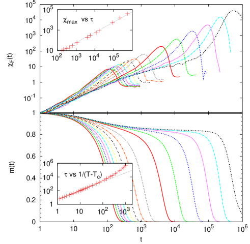
Figure 4: (color online): Dynamical susceptibility (top) and decay of the magnetization $m(t)$ (bottom) in the melting of the 2D 10-state Potts model with $N=250000$ spins. From left to right: $T=0.8$, $0.79$, $0.78$, $0.77$, $0.76$, $0.75$, $0.74$, $0.73$, $0.72$, $0.71$, $0.706$, $0.704$, $0.703$, $0.7025$ and $0.7022$. The insets show the super-exponential divergence of the relaxation time (bottom) and of the maximum susceptibility (top), that is found to grow as $\chi_{\rm max}\propto\tau$.

IV.2 Point-to-set like correlations

We shall now fix the boundaries to be in the fully ordered configuration and study the magnetization they induce for temperature $T\geq T_{c}$. We follow PTS-Exp-Num and consider a box of size $L$ with fixed fully magnetized boundary conditions. We then run a Monte-Carlo simulation, using the Wolff’s cluster algorithm Wolff in order to reach equilibrium, and measure the total magnetization inside the systems for different sizes $L$ and temperatures $T$. The results are shown in Fig. 5. We see clearly a growing point-to-set correlation length that diverges as the transition at $T_{c}$ is approached. Defining the correlation length as the moment when the magnetization falls bellow the plateau (in practice, we used $m<0.8$), we observed that the length grows approximately as $1/(T-T_{c})^{0.8(1)}$, which is not very far from the linear scaling of the size of a critical nucleus (12). Indeed, $\xi(T)$ is nothing but an estimation of the nucleus average size Cavagna in the melting process. As the temperature drops, melting dynamics is initiated by the reversal of larger and larger clusters of spins (the nuclei that will later expand), and the size of these clusters diverges at $T_{c}$.

A word of caution is needed here: we have identified a diverging length scale in first-order transition process. But this length not be confused with the equilibrium correlation length, which does not diverge at a first order transition (in fact it reaches a value of $\approx 7.5$ lattice spacings exactly at the transition in this model, see Janke ). The point-to-set length diverges while the equilibrium correlation one does not.

To echo the discussion in sec. II.3, let us further emphasize that the point-to-set construction we have used is also different from taking first a very large box with ordered boundary conditions and then measuring the magnetization at distance $L$ from the boundaries. Indeed, for box sizes $L\gg\xi$ nucleation is always favorable and the nucleus thus invades almost the whole system. From the data presented in Fig. 5 we can see that the magnetization for $L\gg\xi$ starts to decay as the inverse of the size $L$. This can be understood easily: If the correlation with the boundaries in a very large box is set by a characteristic distance $\ell$, then the local magnetization will be roughly one at distance $d<\ell$ from the boundaries, and roughly zero at distance $d>\ell$. The total magnetization should thus behave as $m\propto\ell/L$ when $L\gg\xi$. The characteristic length $\ell$ is, however, much smaller and unrelated to the point-to-set construction (in fact, it is in the so-called wetting length, which is expected, at least in simple mean field models, to diverge logarithmically at the transition, see for instance BOOKWETTING ). This is a major difference with the mean field case where at the spinodal point, both the correlation length with frozen boundaries in an infinite system (that is, the wetting length) and the length defined by the onset of magnetization in a finite system (that is, the point-to-set length) are equal and diverge in the very same way. This is not true anymore in finite dimensional systems.

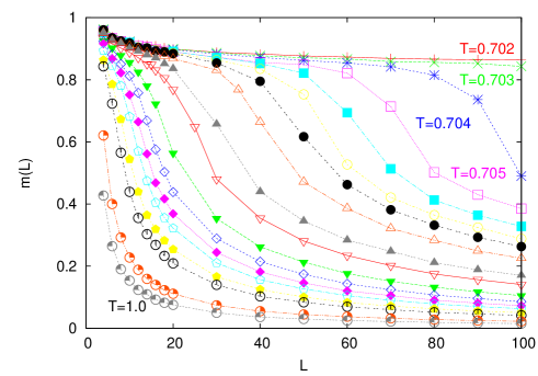
Figure 5: (color online) Equilibrium average magnetization in a box of size $N=L^{2}$ with fully magnetized fixed boundary conditions in the 2D Potts model. These data indicate the growth of the point-to-set length scale as the transition at $T_{c}$ is approached. Defining the correlation length $\xi(T)$ such that $m(\xi)<0.8$, we find that $\xi\propto(T-T_{c})^{-0.8(1)}$, which is reasonably close to the prediction $1/(T-T_{c})$ of nucleation theory .

IV.3 Dynamical heterogeneities

We also computed the dynamical susceptibility $\chi_{F}(t)$, see Fig. 4. Again, it yields the qualitative behaviour of the $\chi_{4}$ observed in glassy systems, meaning that the dynamical heterogeneities are the largest when the susceptibility reaches its maximum and they grow as the temperature is approaching the phase transition. As we are working with a 2D system, visualization is convenient and we thus depict these heterogeneities in Fig. 6.

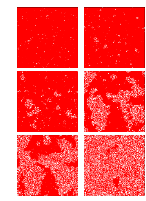
Figure 6: (color online) Nucleation process in the melting of the 2D Potts model with $q=10$ at temperature $T=0.7025$ with $N=1500^{2}$ spins. The red dots are the spins that have the same value as the initial state $S=1$, white are all the other spins. The times are from top to bottom $25000$, $75000$, $120000$, $220000$, $260000$, $380000$. On the second image, we can already recognize some nucleating critical droplets that start to grow fast for larger times. The nucleating droplets percolate between images n. $4$ and n. $5$, this corresponds to the time at which the heterogeneities and the dynamical susceptibility are the largest. The typical size of heterogeneities is much larger than the size of critical nuclei .

Since the melting proceeds via nucleation, one might think that the maximum of the $\chi_{F}(t)$ denotes the volume of the critical droplet (12). This is not the case, in fact the volume described by the maximum of $\chi_{F}$ is much larger than the critical nucleus size. This is clearly visible in the simulations depicted in Fig. 6, where the size of a typical critical nucleating droplet is about $10^{2}$, while the typical size of the correlated regions close to the maximum of the $\chi_{F}$ is about $100^{2}$.

The reason beyond this is simple and illustrates well the nucleation and growth mechanism. As described in Sec. III, after a time of $O\left(\tau_{\rm relax}\right)$, grown droplets will touch each other and percolate; this is the moment at which the maximum of the $\chi_{F}$ arises, and we expect that this maximum thus behaves algebraically with the relaxation (and the nucleation) time so that $\chi_{F}\propto\tau^{\alpha}$, which is indeed what we find in the inset of Fig. 4. This shows that the nature of the static and the dynamic length scale is completely different, and that the dynamical susceptibility can probe much larger scales. The first one probes the length associated with critical nuclei while the second one depends on the growth process. Note that the exponential divergence of $\chi_{F}$ (with respect to the temperature difference as the critical point is approached) compares well with what is observed in many models with kinetically constraint or facilitated dynamics Chi4_kinetic_1 ; Chi4_kinetic_2 ; Chi4_kinetic_3 .

Given the simplicity of its origin, a law $\chi_{F}\propto\tau^{\alpha}$ should indeed be quite generic for systems with nucleation and growth. However, the value of the exponent $\alpha$ depends on the type of growth and on the precise properties of the system. The growth process of nuclei can be in principle much slower in system with disorder (where, due to the pinning of the interface, activation is again necessary to grow the nuclei) with respect to the relatively fast process observed here, and its interplay with nucleation can be more complicated. In fact, the growth can probably be so slow that the two length scales might be comparable, and this will be investigated in a companion paper US-PART-II .

V Differences between bulk melting and glassy dynamics

So far we concentrated on the analogies between glassy dynamics and bulk melting, it is time to list several key differences. First of all, the analogy does not extend to non-equilibrium properties such as aging in glasses Kurchan . We are comparing here the melting process with the equilibrium-initialized dynamics in the glassy systems, but the out-of-equilibrium behaviour of glasses is very different. But let us concentrate on the differences in the dynamics from equilibrium.

A crucial point is that there is no latent heat associated to the glass transition, as the energy is continuous, while there is a latent heat in a general first-order transition (for instance both in the ferromagnetic $p$-spin model and the 2D Potts model we discussed in this paper). To smear away this difference one should consider a first order transition driven purely by entropy, if the energy is continuous at the first order phase transition then there is no latent heat. This is the case for instance in a system of hard spheres.

Another major difference in the dynamical behaviour is that the melting process happens once for all. When the system has melted, it stays in the liquid phase. However, the equilibrium glassy dynamics is a stationary process which is time-translationally invariant. This is why the equivalent of the nucleation theory in glasses, the so-called mosaic picture AdamGibbs ; KW1 ; KW2 ; KTW ; BiroliBouchaud , is more complicated (and not yet fully understood).

Our results seem, however, to point towards the glass transition being a melting of some special sort. In the glass problem, following the ideas of Goldstein Goldstein , we can assume that we have a more complicated landscape, with many local minima. The glassy dynamics consists of a continuous and stationary melting of one minima to another one. This view is precisely the one adopted in the mosaic picture and in the RFOT KW1 ; KW2 ; KTW ; BiroliBouchaud .

The comparison between melting and glassy dynamics will be pushed beyond a simple analogy in a companion paper US-PART-II , where we show that in a certain class of spin systems (both mean-field and finite dimensional ones) with a first order phase transition, one observes a purely entropic transition and the melting dynamics is a in fact equivalent to the equilibrium dynamics. In order to do so we explore properties on the Nishimori line Nishimori-Original ; Nishimori ; Ozeki1 ; Ozeki2 and study consequences of such a mapping for the physics of the glass transition.

VI Discussion

In this paper we explored analogies between the bulk melting dynamics above a first order phase transition and the equilibrium glassy dynamics. We showed that many properties associated with the dynamics of structural glass formers are already present in the melting case. We have investigated several features of modern theory of super-cooled liquids — such as the diverging relaxation time, the plateau in the correlation function, dynamical heterogeneities related to the dynamical susceptibility $\chi_{4}$, the point-to-set correlations — and showed that they all can be easily recovered and understood in a much simpler setting of systems with a first order phase transition. In particular the dynamical —or mode-coupling— transition corresponds to the spinodal point, while the Kauzmann transition corresponds to the first order ferromagnetic phase transition.

Noticing similarities between the glass transition and the first order one is of course not new. In fact, it is somehow implicit in the random first order theory of glasses KW1 ; KW2 ; KTW , where according to the mosaic picture every glassy state melts into another one and so on. The notion of nucleation stands at the roots of the theory deriving the Adam-Gibbs law and the mosaic theory is nothing but the counter-part of nucleation theory for glassy transitions. The construction of Franz and Parisi FranzParisi and the earlier work of KT are attempts to root the theory of the glassy transition into a first-order setting. The recent work of CavagnaAgain also accentuates the analogy, and the very definition of the point-to-set correlation was recently proposed as a tool to investigate nucleation in systems with a generic first order transition Cavagna , and this is by far not an exhaustive list. The bottom-line of our approach here is that it is rather interesting to take this analogy literally, to concentrate on the simpler melting problem, and to understand in detail its glassy aspects. We believe this approach can be interesting for the bulk melting problem per se.

Before concluding, let us make a last comment. The random first order theory is not fully accepted as a good theory of the glass transition. Without taking a position on the question whether RFOT is the good theory for the glass transition or not, we want to point out here that many of the criticisms of RFOT apply equally to systems with an ordinary first order phase transition. Imagine for a moment that we would study melting dynamics without knowing about the underlying first order phase transition. In this case researchers could be trying different fits to extrapolate the divergence of the melting time at a finite or zero temperature hecksher2008little . They could also criticize the use of ill-defined metastable states Langer ; Chi4_kinetic_1 ; Wyart . Mean-field theories would predict a spinodal line with a power-law divergence MCT ; MCT2 , and the crossover to finite dimensional behaviour could be thought of as a mysterious one BiroliBouchaud09 . There would be some claims that mean-field theories do not incorporate geometric properties and hence are not very relevant to finite dimensional systems Langer . Some would concentrate on the heterogeneous fluctuations in the decay of the order parameter, and on the peculiar shape of critical nucleating droplets as the central object of interest PhysRevLett.80.2338 ; claiming at the same time that there is no need to think about thermodynamics Ludo and that melting should be modeled with purely dynamic systems with simple rules Chandler . In cases of systems such as diamond the melting transition might even be not considered at all because the true equilibrium state is simple carbon — just as the crystal is always the true equilibrium state in glass forming systems CRYSTAL . Luckily, first order phase transitions are much more established (since in this case, contrary to what happens in glasses, we can equilibrate at low temperatures), hence the answers to the above arguments are mostly well understood. Still, this shows that starting from a mean-field analysis and correcting it with nucleation-like arguments, as is done in RFOT, is not such a bad strategy a priori.

Finally, a lesson from this study is that one should maybe look back to the first order phase transitions with the eyes of glassy phenomenology, both from an experimental and theoretical point of view. The following questions are for instance appealing: How do the static and dynamic lengths behave in other models with first order transitions (with or without disorder)? What does the mode-coupling approximation predict for a first order phase transition? Can all the recent experimental investigations of static and dynamic length scales in glass formers be repeated in a first order melting process? The way a solid flows under shear is clearly related to the melting mechanism GiulioLast , does the dynamical susceptibility diverge as a power of the relaxation time as well?

These questions are particularly appealing in the context of bulk melting in super-heated solids Superheating . It would be for instance interesting to apply the dynamical correlation and susceptibility analysis of sections II.3 and IV.3 in order to identify dynamical heterogeneities (which seem indeed to be present in this problem, see for instance SuperANDHetero ). This could also help to understand the interplay between nucleation and growth in melting processes. Other common behaviour can be identified upon inspection; compare for instance the string-like motion STRING observed in glassy dynamics with the highly correlated ring and loop atomic motions behaviour observed in bulk melting MO (and more generally with the stringy nuclei observed close to pseudo-spinodal during first-order transition KLEIN ). Another example is given by the behaviour of the shear modulus: according to a recent work within the RFOT, it is predicted to vanish continuously at the mode-coupling transition point in glasses MARC , a statement clearly reminiscent of the Born criterion BORN that defines the spinodal point of superheated solid as the moment where shear modulus is going to zero. Finally, studying the system with respect to frozen boundary conditions as in section IV.2 should also be interesting in order to estimate nucleation barriers numerically in the spirit of Cavagna , and to investigate the much studied problem of the limit of the super-heated state.

To conclude, there is a lot to learn on the crossroad between glasses and first order melting, and we hope our article will trigger new works in this direction. This will be further accentuated in a companion article where we provide a set of models where the melting process is exactly equivalent to its equilibrium dynamics US-PART-II and where we show that the mean-field theory of the glass transition is mappable to a (special) melting problem.

Appendix: The ferromagnetic $p$-spin model

In this appendix, we remind how to solve the static and the dynamic behaviour of the fully connected ferromagnetic $p$-spin model defined by Hamiltonian (1) with $J=1/N^{p-1}$.

.1 The thermodynamic solution

In order to compute the free energy as function of magnetization, we consider the Hamiltonian (1) with an external magnetic field $h$, it then becomes $H=-N(m^{p}+hm)$. Applying the integral representation of the delta function, one finds

$$Z(h) =\sum_{\{S_{i}\}}\int{\rm d}m\,\delta(Nm-M(\{{\vec{S}\}}))\,e^{\beta N\left[m^{p}+hm\right]}$$

$$= \int\!\!{\rm d}m\,{\rm d}\lambda\,e^{\beta N(m^{p}+hm)\!-\!N\!\lambda m+N\log{(2\cosh{\lambda})}}.$$

The saddle point condition imposes that $\lambda=\beta pm^{p-1}+\beta h$ and therefore

$$Z(h)=\int{\rm d}m\,e^{-\beta Ng(m,\beta,h)}$$ (17)

with

$$g(m,\beta)=(p-1)m^{p}-\frac{1}{\beta}\log{[2\cosh{\left(\beta pm^{p-1}+\beta h\right)}]}\,.$$ (18)

The self-consistent equation on $m$ thus reads

$$m=\tanh{\left(\beta pm^{p-1}+\beta h\right)}\,.$$ (19)

We are interested in the free energy as a function of the equilibrium magnetization $m$. This is obtained by the Legendre transform of eq. (18), that is, by $f(m,\beta)=g(h^{*},\beta,m)+h^{*}m$, where $h^{*}$ is given by the condition (19). It yields finally

$$\beta f(m,\beta)=-\beta m^{p}-\log{\left[2\cosh{\,(\text{atanh}{\,m})}\right]}+{m~{}\text{atanh}(m)}\,.$$ (20)

This formula was used to produce Fig. 1. For $p=3$, this solution yields first-order phase transition at $\beta_{c}=0.67209$. The low temperature phase, however, is locally stable until the spinodal point at $\beta_{s}=0.57217$.

.2 The Bethe-Peierls solution

Consider the $p$-spin model on a tree with coordination number $c$. In this case, one can write an iterative recursion using the Bethe-Peierls strategy that relates the magnetization at level $l+1$ with the one at level $l$ XORSAT

$$m_{l+1}=\tanh{\left\{(c-1){\rm arctanh}{\left[\tanh{(\beta J)}m_{l}^{p-1}\right]}\right\}}\,.$$ (21)

Let us now take the limit of a very large connectivity and use $J=p/c$. In this limit

$$m_{l+1}=\tanh{\left(p\beta m_{l}^{p-1}\right)}\,.$$ (22)

The stationarity condition of this equation leads to eq. (19). This formulation allows to define a correlation length as is done in sec. II.3.

.3 Solving the dynamics of the melting process

We define the Glauber dynamics as follow: At each interval of time $1/N$, we pick up one spin, and set it plus with probability $p_{+}={(1+\tanh{\beta h})}/2$ and minus with probability $p_{-}={(1-\tanh{\beta h})}/2$, where $h=pm^{p-1}$ is the local field on the spin, that is conveniently the same for every spin. To compute the evolution of magnetization and susceptibility (7), we define $P(t,M)$ as the probability (over different realizations of the dynamics) that the value of the magnetization is $M$ at time $t$, where $-N\leq M\leq N$. Its averaged value per site reads

$$m(t)=\frac{1}{N}\int_{0}^{1}P(t,M)M{\rm d}m\,,$$ (23)

and the average susceptibility is

$$\chi(t)=\frac{\beta}{N}\left\{\int_{0}^{1}P(t,M)M^{2}{\rm d}m-\left[\int_{0}^{1}P(t,M)M{\rm d}m\right]^{2}\right\}\,,$$ (24)

where $M=Nm$. The master equation for $P(t,M)$ reads

$$P(t+{\rm d}t,M)=\frac{N+(M+2)}{2N}\,p_{-}(M+2)\,P(t,M+2)$$

$$+\frac{N-(M-2)}{2N}\,p_{+}(M-2)\,P(t,M-2)$$

$$+\left[\frac{N+M}{2N}p_{+}(M)+\frac{N-M}{2N}p_{-}(M)\right]P(t,M)\,.$$ (25)

The average magnetization at time $t+{\rm d}t$ is thus

$$Nm(t+{\rm d}t)=\int_{0}^{1}P(t,M){\rm d}m\left[M-m+\tanh{(\beta pm^{p-1})}\right]\,.$$ (26)

Considering that fluctuations in $m$ are $O(1/\sqrt{N})$, this leads to the differential equation (4).

The evolution of the dynamical magnetic susceptibility is computed in a similar manner. Using (25), the second moment of $M$ reads

$$\int_{0}^{1}M^{2}P(t+{\rm d}t,M){\rm d}m=\int_{0}^{1}M^{2}P(t,M){\rm d}m$$ (27)

$$+ \int_{0}^{1}2MP(t,M)\left[-m+\tanh{(\beta pm^{p-1})}\right]{\rm d}m$$

$$- \int_{0}^{1}2P(t,M)\left[m\tanh{(\beta pm^{p-1})}-1\right]{\rm d}m\,.$$

Now from the definition of $\chi(t)$ after collection all the terms from (26) and (27) we get

$$N \chi(t+{\rm d}t)/\beta=N\chi(t)/\beta$$

$$+ \int_{0}^{1}2(M-\langle M\rangle)P(t,M)\left[-m+\tanh{(\beta pm^{p-1})}\right]{\rm d}m$$

$$+ 2\langle m\tanh{(\beta pm^{p-1})}\rangle-2-\langle-m+\tanh{(\beta pm^{p-1})}\rangle^{2}\,.$$

The remaining integral on the r.h.s. can be rewritten using a Taylor series around $\langle m(t)\rangle$. Finally we obtain the following differential equation for $\chi(t)$

$$\frac{{\rm d}\chi(t)}{{\rm d}t}=-2\chi(t)+2\frac{\beta p(p-1)m(t)^{p-2}}{\{\cosh{[\beta pm(t)^{p-1}]}\}^{2}}\chi(t)$$ (28)

$$+ 2\beta-\beta m^{2}(t)-\beta\left\{\tanh{[\beta pm(t)^{p-1}]}\right\}^{2}\,.$$

Equations (4) and (28) can be numerically integrated together, and yield the results in Fig. 2.

References

- (1) P. G. Debenedetti and F. H Stillinger, Nature 410, 6825 pp. 259-267 (2001).
- (2) M. D. Ediger, C. A. Angell, S. R. Nagel, J. Phys. Chem. 100, 13200 (1996).
- (3) C. A. Angell, Journal of Physics and Chemistry of Solids 49, n. 8, 863-871 (1988).
- (4) H. Vogel, Phys. Z. 22, 645 (1921). G. S. Fulcher, J. Am. Ceram. Soc. 8, 339 (1925).
- (5) W. Kauzmann, Chem. Rev., 1948, 43 (2), 219 (1948).
- (6) G. Adam, J. H. Gibbs, J. Chem. Phys. 43, 139–146 (1965).
- (7) S. Franz and G. Parisi, J. Phys.: Condens. Matter 12, 6335 (2000).
- (8) C. Toninelli et al., Phys. Rev. E 71, 041505 (2005).
- (9) E. R. Weeks et al., Science 287, 627-631 (2000).
- (10) J.-P. Bouchaud and G. Biroli, J. Chem. Phys. 121, 7347–7354 (2004).
- (11) A. Montanari and G. Semerjian, J. Stat. Phys. 124, 103 (2006).
- (12) A. Montanari and G. Semerjian, J. Stat. Phys. 125, 23 (2006).
- (13) A. Cavagna, T. S. Grigera and P. Verrocchio, Phys. Rev. Lett. 98, 187801 (2007). G. Biroli, J.-P. Bouchaud, A. Cavagna, T. S. Grigera and P. Verrocchio, Nature Physics 4, 771 (2008).
- (14) T. R. Kirkpatrick and D. Thirumalai, Phys. Rev. Lett. 58, 2091 (1987). T. R. Kirkpatrick and D. Thirumalai, Phys. Rev. B 36, 5388 (1987).
- (15) T. R. Kirkpatrick and P. G. Wolynes, Phys. Rev. A 35 3072 (1987).
- (16) T. R. Kirkpatrick and P. G. Wolynes, Phys. Rev. B 36 8552 (1987).
- (17) T. R. Kirkpatrick, D. Thirumalai, P. G. Wolynes, Phys. Rev. A 40, 1045–1054 (1989).
- (18) M. Mézard and G. Parisi, Phys. Rev. Lett. 82, 747 (1999).
- (19) B. Derrida, Phys. Rev. Lett. 45, 79 - 82 (1980). B. Derrida, Phys. Rev. B 24, 2613 - 2626 (1981).
- (20) D. J. Gross and M. Mézard, Nucl. Phys. B 240, 431 (1984).
- (21) F. Ricci-Tersenghi, M. Weigt and R. Zecchina, Phys. Rev. E 63, 026702 (2001). S. Franz et. al. Europhys. Lett. 55, 465-471 (2001).
- (22) M. Mézard, G. Parisi, and M. A. Virasoro, Spin-Glass Theory and Beyond, Lecture Notes in Physics Vol. 9 (World Scientific, Singapore, 1987).
- (23) W Gotze, J. Phys.: Condens. Matter 2 SA201 (1990),
- (24) S. P. Das, Rev. Mod. Phys. 76, 785 (2004).
- (25) G. Biroli and J.-P. Bouchaud, Europhys. Lett. 67, 21 (2004).
- (26) L. Cugliandolo and J. Kurchan, Phys. Rev. Lett. 71, 173 (1993).
- (27) J.-P. Bouchaud et al., Physica A 226 243 (1996). J.-P. Bouchaud et al., in Spin Glasses and Random Fields, edited by A. P. Young (World Scientific, Singapore, 1998).
- (28) A. Cavagna, I. Giardina and G. Parisi, J. Phys. A :Math. Gen. 34 5317-5326 (2001).
- (29) J.S. Langer, Phys. Today 8–9 (2007).
- (30) G. Biroli and J.-P Bouchaud, arXiv:0912.2542 (2009).
- (31) F. Krzakala and L. Zdeborová, On Glassy dynamics as a Melting process in preparation.
- (32) H. Nishimori, Prog. Theor. Phys. 66, 1169 (1981).
- (33) H. Nishimori, Statistical Physics of Spin Glasses and Information Processing: An Introduction (Oxford, 2001).
- (34) J. G. Dash, Rev. Mod. Phys. 71, 1737 (1999).
- (35) W. G. Hoover and F. H. Ree, J. Chem. Phys. 49, 3609 (1968).
- (36) F. Y. Wu, Rev. Mod. Phys. 54, 235–268 (1982).
- (37) R. W. Cahn, Nature (London) 273, 491 (1978);
- (38) K. Chattopadhyaya and R. Goswamib, Prog. Mat. Sci. 42 287 (1997).
- (39) J. Frenkel, Kinetic Theory of Liquids (Clarendon, Oxford) (1946).
- (40) I. N. Stranski, Naturwissenschaften 28, 425 (1942).
- (41) J. Daeges et al., Phys. Lett. A 119, 79 (1986), L. Grabaek et al., Phys. Rev. B 45, 2628 (1992). L. Zhang et al., Phys. Rev. Lett. 85, 1484–1487 (2000) C. W. Siders et al., Science 286, 1340 (1999); A. Rousse et al., Nature (London) 410, 65 (2001).
- (42) Z. H. Jin, Phys. Rev. Lett. 87, 055703 (2001). F. Delogu, J. Phys. Chem. B 2006, 110, 3281-3287 (2006).
- (43) T. D. Lee and C. N. Yang , Phys. Rev. 87, 410–419 (1952).
- (44) K. Binder, Rep. Prog. Phys. 50 783-859 (1987).
- (45) K. Binder, Phys. Rev. B 8, 3423–3438 (1973).
- (46) M. Iwata, S. Sasa, arXiv:1002.4239v1 (2010).
- (47) Statistical mechanics of membranes and surfaces, D. Nelson, T. Piran and S. Weinverg editors. See for instance the discussion of D. Nelson in chapter 1 and the figure 2a.
- (48) J. S. Langer, Phys. Rev. Lett. 21, 973 (1968). J. S. Langer, Ann. Phys. (N.Y.) 54, 258 (1969).
- (49) A. Cavagna, Physics Reports, 476, 51 (2009)
- (50) J. W. Gibbs, Collected Works, vol. 1 (Yale U.P., New Haven, Conn., 1948).
- (51) A. N. Kolmogorov, Bull. Acad. Sci URSS (cl. Sci. Math. Nat.) 3, 355 (1937). W. A. Johnson and R. F. Mehl, Trans. Am. Inst. Min., Metall. Pet. Eng. 135, 416 (1939). M. Avrami, J. Chem. Phys. 7, 1103 (1939); 8, 212 (1940).
- (52) U. Wolff, Phys. Rev. Lett. 62, 361 (1989).
- (53) C. Cammarota and A. Cavagna, Journal of Chemical Physics 127, 214703 (2007).
- (54) W Janke, S Kappler, EPL 31 345, 1995.
- (55) M. R. Evans, J. Phys.: Condens. Matter 14, 1397–1422 (2002).
- (56) C. Toninelli, G. Biroli and D. Fisher, Phys. Rev. Lett. 96, 035702 (2006).
- (57) L. Berthier, Phys. Rev. Lett. 91, 055701 (2003).
- (58) F. Sausset, G. Biroli, J. Kurchan, arXiv:1001.0918 (2010).
- (59) S. Franz, G. Parisi, Phys. Rev. Lett. 79, 2486 (1997).
- (60) C. Cammarota et al., arxiv:1001.2539 (2010).
- (61) M. Goldstein, J. Chem. Phys. 51, 3728 (1969).
- (62) Y. Ozeki, J. Phys. A: Math. Gen. 28, 3645 (1995).
- (63) Y. Ozeki, J. Phys.: Condens. Matter 9, 11171 (1997).
- (64) T. Hecksher et al.; Nature Physics, 4, 737 (2008). G. B. McKenna, Nature Physics 4, 673 (2008).
- (65) M. Wyart, arXiv:0911.4059 (2009).
- (66) C. Donati et al., Phys. Rev. Lett., 80, 2338 (1998).
- (67) L. Berthier and J. P. Garrahan, Phys. Rev. E 68, 041201 (2003).
- (68) J. P. Garrahan and D. Chandler, Phys. Rev. Lett. 89, 035704 (2002).
- (69) A. Donev, F. H. Stillinger, S. Torquato, Phys. Rev. Lett. 96, 225502 (2006).
- (70) C. Donati et al, Phys. Rev. Lett. 80, 2338–2341 (1998).
- (71) X-M Bai and M. Li, Phys. Rev. B 77, 134109 (2008).
- (72) H. Wang, H. Gould and W. Klein, Phys. Rev E 76, 031604 (2007)
- (73) H. Yoshino and M. Mezard, arXiv:1003.3039, to appear in Phys. Rev. Lett.
- (74) M. Born, J. Chem. Phys. 7, 591 (1939); Proc. Cambridge Philos. Soc. 36, 160 (1940).