Glassy dynamics as a melting process
On melting dynamics and the glass transition, Part II

Abstract

There are deep analogies between the melting dynamics in systems with a first order phase transition and the dynamics from equilibrium in super-cooled liquids. For a class of Ising spin models undergoing a first order transition – namely $p$-spin models on the so-called Nishimori line – it can shown that the melting dynamics can be exactly mapped to the equilibrium dynamics. In this mapping the dynamical —or mode-coupling— glass transition corresponds to the spinodal point, while the Kauzmann transition corresponds to the first order phase transition itself. Both in mean field and finite dimensional models this mapping provides an exact realization of the random first order theory scenario for the glass transition. The corresponding glassy phenomenology can then be understood in the framework of a standard first order phase transition.

There is still no agreement on what is the fundamental principle behind the experimentally observed abrupt change in the relaxation time of super-cooled liquids when the temperature is lowered GLASS-GEN:1 ; GLASS-GEN:2 ; ANGELL . Many scenarios and theories have been proposed over the time to describe the nature of glasses, and over the last few years the theoretical research has been concentrated on the following questions. Is there an underlying critical phenomenon behind the glass transition or not? Is the glass transition a thermodynamic or a purely dynamic notion? What is the correct theory of super-cooled liquids?

The most remarkable experimental fact in the phenomenology of super-cooled liquids is the extremely fast rise of the relaxation time $\tau$, that increases by several orders of magnitude as the temperature is decreased by only a few percents. The relaxation time is traditionally fitted (and well approximated) by the Vogel-Fulcher-Talman law $\tau\propto\exp{[A/{\left(T-T_{VFT}\right)}]}$ VogelFulcher . The extrapolated temperature $T_{VFT}$ is found to be close the Kauzmann temperature $T_{K}$ where the extrapolated entropy of the super-cooled liquid becomes smaller than the entropy of the crystal Kauzmann , a fact that has led to speculations on the existence of an ideal —yet impossible to observe in finite time— glass transition at $T_{K}\approx T_{VFT}$. Another fact pointing in the direction of an ideal glass transition is the Adam-Gibbs AdamGibbs relation $\tau\propto\exp{[C/\Delta S(T)]}$, where $\Delta S(T)$ is the difference between the entropy of the crystal and the liquid, this gives a further link between thermodynamic and dynamic behaviour.

In the last decade, a lot of attention has been devoted to growing length scales. In most theories the slower-than-exponential relaxation time in fragile super-cooled liquids follows from the fact that larger and larger regions become correlated as the temperature is lowered, so that larger ensembles of particles have to be rearranged collectively to relax the system into equilibrium. However, the standard static correlation function does not show any sign of such a growing correlation length, and more complex correlation functions thus have to be considered. Two length scales that are observed to grow significantly when the temperature is lowered have been now identified. The first is a purely dynamic length associated to spacial heterogeneities in the dynamics Silvio ; DynBB ; DynHS . The second length is an equilibrium one associated with the correlation of a sub-system with its frozen boundaries BiroliBouchaud ; DynamicBethe ; PointToSet . The existence of diverging correlation lengths points towards the glass transition being a critical phenomena.

Is there really a genuine glass transition? Are the time and length scales really diverging when approaching the glass transition or are they only growing? A definitive answer on these questions is difficult to obtain as both simulations and experiments are faced with the extremely slow dynamics. According to the random first order theory (RFOT) of the glass transition KT ; KW1 ; KW2 ; KTW ; GlassMezardParisi , the above mentioned time and length scales have a genuine divergence at the ideal glass transition temperature, although the RFOT theory is not free from criticisms (see for instance Langer ; BiroliBouchaud09 and references therein).

In a companion paper US-PART-I we have discussed that a large part of the glassy phenomenology also appears in the melting process of a fully ordered phase above an ordinary first order phase transition. The bottom-line of the analysis is that when the ordered system is brought at higher temperature than the melting point, it is inside a metastable state from which it needs to escape, and this is associated to diverging time and length scales analog to those we just discussed for glasses, except that in this case the existence of a genuine transition is doubtless. There are, however, also important differences between melting above an ordinary first order phase transition and the glassy dynamics.

In this work we will show that for a class of spin models, both in mean field and finite dimensional systems, these differences are washed away and the melting dynamics can be shown to be exactly equivalent to the equilibrium dynamics above the first order phase transition. These models are nothing but variants of the Ising $p$-spin models that have inspired the RFOT theory REM ; P-SPIN ; XORSAT , and most of our approach is built on the construction of Nishimori and collaborators Nishimori-Original ; Nishimori , in particular Ozeki Ozeki1 ; Ozeki2 . Our results are two-folds: (1) we show that the standard mean-field approach to the glass transition is exactly mappable to a melting problem of some sort; (2) we show that there exists a set of finite dimensional models where the melting process is equivalent to the glassy dynamics in a glass-forming liquid, and that the existence of a first-order transition for the melting problem implies the existence of a RFOT-like transition for the glass. Our results offer an alternative and potentially fruitful way of looking at the glass transition problem, all from a theoretical, numerical and experimental point of view. In particular, many questions about the glass transition may be recasted into the more familiar and simpler to describe properties of first order phase transitions.

The paper is organized as follows: In the section I we present a class of disordered Ising spin models and concentrate on a special line in the temperature/disorder plane —the Nishimori line— where the melting problem is equivalent to the equilibrium dynamics. In section II we discuss the mean-field version of these models. In section III we concentrate on a three-dimensional case. We summarize and discuss our results in the last section.

I When melting is equivalent to equilibrium dynamics

Following the ideas of Edwards and Anderson, a large part of the progress in the theory of glasses have originated in studies of spin glasses EA ; MPV ; Hertz . In particular, the Ising $p$-spin glass REM ; P-SPIN ; XORSAT provides a mean-field theory for the structural glass transition KT ; KW1 ; KW2 ; KTW , which is an exact realization of the early landscape picture of Goldstein Goldstein . Here we shall follow this path, although we will not restrict ourself to the mean field theory.

Consider the $p$-spin Hamiltonian, with $p=3$ we have

$${\cal H}=-\sum_{ijk}J_{ijk}S_{i}S_{j}S_{k},$$ (1)

where the sum is over some triplets of spins (the precise details on how the triplets are chosen depends on the geometry of the problem: mean-field lattice, finite-dimensional grid, etc.), and the interactions $J_{ijk}$ are quenched random variables taken from the distribution

$$P_{\rho}(J_{ijk})=\rho\delta(J_{ijk}-1)+(1-\rho)\delta(J_{ijk}+1)\,,$$ (2)

where $\rho$ can vary from $\rho=1/2$ (the spin glass case: $J_{ijk}=\pm 1$ with equal probability) to $\rho=1$ (the ferromagnetic case with $J_{ijk}=1$).

Consider first the pure ferromagnetic model with $\rho=1$. The ferromagnetic many-body interaction models undergo usually a first order transition, both in mean field US-PART-I ; XORSAT and in finite dimension (see the simulations of the plaquette models in Plaquette_L ; Plaquette_B ; STAR_model ). At high temperature the system is in a paramagnetic/liquid state, while for low temperature it is in a ferromagnetic/crystal one, and a first order transition at $T_{F}$ separates the two.

The dynamical behavior of the ferromagnetic many-body interaction models, on the other hand, reproduces many aspects of super-cooled liquids and their glass transition. In particular, crystallization at $T_{F}$ seems to be easily avoidable when cooling down from a large temperature, and the super-cooled liquid so obtained has all the desired glassy phenomenology. There are, however, several problems (actually common to most glassy systems) that prevent analytical and conceptual progress:

(1) The fact that below the ferromagnetic/melting temperature $T_{F}$ the true equilibrium state is given by the ferromagnet/crystal makes always any statement on equilibrium super-cooled liquid delicate, to say the least. Any discussion involving the description of the putative ideal glass transition at temperature $T_{K}<T_{F}$ is plagued by this problem, since there will always be a temperature beyond which the nucleation time towards the crystal will be larger than the relaxation time in the super-cooled liquid phase Kauzmann ; STAR_model . It would thus be interesting to find a model with $T_{K}=T_{F}$ so that the divergence of the equilibration time in the liquid phase could be well defined.

(2) Glass formers are known to be hard to simulate, since the time to find an equilibrium configuration grows faster than exponentially with the temperature. It would be really convenient to have an equilibrium configuration to start the simulation with at all temperatures.

(3) Usually in glassy models, it is really difficult to make any statement which is not coming from numerical simulations. It would be really convenient to have some analytical results and guarantees of genuine phase transitions and divergences.

Quite surprisingly, there is a conceptually simple, and rigorous way, to avoid the above difficulties for a class of Ising $p$-spin models if one works on the so-called Nishimori line and this is the main topic of this paper.

I.1 Physics on the Nishimori line

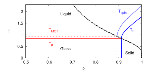
Figure 1: (color online) Phase diagram of the mean field $3$-spin Ising spin glass model on a Bethe lattice with coordination $c=5$ and a fraction of ferromagnetic couplings $\rho$. In the spin glass case ($\rho=1/2$) —which is the starting point of the random first order theory of the glass transition— there is a mode-coupling type transition at $T_{\rm MCT}=0.936$ (dashed red) while the thermodynamic glass transition is at $T_{K}=0.849$ (full red). In the purely ferromagnetic case ($\rho=1$) the model undergoes a first order ferromagnetic phase transition at $T_{F}$. The ferromagnetic transition extends to lower $\rho$ (lower blue line), as well as the spinodal line of the ferromagnetic phase $T_{\rm spin}$ (upper blue line). Using a gauge transformation we show that the relaxation dynamics for all $T\geq T_{K}$ in the spin glass case is strictly equivalent to the melting dynamics starting from all spins up, $S_{i}=1$, on the Nishimori line, eq. (3), (the black line crossing the diagram from upper left to lower right).

As discovered by Nishimori Nishimori-Original ; Nishimori , there is a special line, the Nishimori line (NL), in the temperature-disorder phase diagram where many results can be established rigorously, on any lattice and thus in any dimension. Following Nishimori-Original ; Nishimori , we start by recognizing that eq. (2) can be rewritten as

$$P_{\rho}(J_{ijk})=\frac{e^{K_{\rho}J_{ijk}}}{2\cosh K_{\rho}}\text{~{}~{}~{}with~{}~{}~{}}\emph{e}^{2K_{\rho}}=\frac{\rho}{1-\rho}\,.$$ (3)

The Nishimori line in the plane $(T,\rho)$ is defined by $K_{\rho}=\beta$ (see Fig. 1 for an explicit example).

Consider a given quantity of interest $A$, say the free energy, the energy or the magnetization, that depends on the realization of the disorder $\{{J_{ijk}\}}$, on the inverse temperature $\beta$, and in general also on the spin configuration $\{S_{i}\}$. As is usual for random systems, we want to consider the average of this quantity over the disorder parameterized by the variable $\rho$.

$$[A]_{\rho}\equiv\sum_{\{J_{ijk}\}}A(\{J_{ijk}\},\{S_{i}\},\beta)\prod_{ijk}\frac{\emph{e}^{K_{\rho}J_{ijk}}}{2\cosh K_{\rho}}\,.$$ (4)

Following again Nishimori , we consider a new set of Ising ($\pm 1$) variables $\{{\sigma_{i}\}}$ and the following gauge transformation

$$S_{i} = \tilde{S}_{i}\sigma_{i}\,,$$ (5)

$$J_{ijk} = \tilde{J}_{ijk}\sigma_{i}\sigma_{j}\sigma_{k}\,.$$ (6)

It is easy to check that this leaves the Hamiltonian invariant, i.e. ${\cal H}(\{S_{i}\},\{J_{ijk}\})={\cal H}(\{S_{i}\sigma_{i}\},\{J_{ijk}\sigma_{i}\sigma_{j}\sigma_{k}\})$. We now apply the gauge transformation and obtain:

$$[A]_{\rho}=\sum_{\{\tilde{J}_{ijk}\}}\frac{\emph{e}^{K_{\rho}\sum_{ijk}\tilde{J}_{ijk}\sigma_{i}\sigma_{j}\sigma_{k}}}{2^{M}(\cosh{K_{\rho}})^{M}}$$

$$A(\{\tilde{J}_{ijk}\sigma_{i}\sigma_{j}\sigma_{k}\},\{\tilde{S}_{i}\sigma_{i}\},\beta)\,,$$ (7)

where $M$ is the number of interactions. Note that the set of values over which is performed the sum $\sum_{J_{ijk}}$ and $\sum_{S_{i}}$ does not change under the transformation either. We now average quantity $[A]_{\rho}$ over all the $2^{N}$ possible choices of the gauge transformation $\{\sigma_{i}\}$ to obtain:

$$[A]_{\rho}=\frac{1}{2^{N}(\cosh K_{\rho})^{M}}\sum_{\{J_{ijk}\}}\frac{1}{2^{M}}$$

$$\sum_{\{\sigma_{i}\}}\,\emph{e}^{-K_{\rho}{\cal H}(\{\sigma_{i}\})}A(\{J_{ijk}\sigma_{i}\sigma_{j}\sigma_{k}\},\{S_{i}\sigma_{i}\},\beta)\,.$$ (8)

At this point, one recognizes that the denominator of the first term is nothing but the annealed average of the partition sum for $\rho=1/2$, and the second term is the disorder average of $A\exp{(-K_{\rho}{\cal H})}$ for $\rho=1/2$. In other words

$$[A\,]_{\rho}=\frac{\left[\sum_{\{\sigma_{i}\}}\,\emph{e}^{-K_{\rho}{\cal H}(\vec{\sigma})}A(\{J_{ijk}\sigma_{i}\sigma_{j}\sigma_{k}\},\{S_{i}\sigma_{i}\},\beta)\right]_{\frac{1}{2}}}{\left[Z\left(K_{\rho}\right)\right]_{\frac{1}{2}}}\,.$$ (9)

If we are on the Nishimori line $K_{\rho}=\beta$, we recognize the right hand side to be the annealed thermodynamic average of the quantity $A$. If $A$ itself is a gauge invariant thermal average of some quantity then from (9) follows that on any lattice the quenched thermodynamic average on the Nishimori line is equal to the annealed thermodynamic average in the fully disordered case ($\rho=1/2$).

Let us denote $Z(\{J_{ijk}\},K_{\rho})$ the partition function for a given realization of disorder $\rho$ and inverse temperature $K_{\rho}$. We denote the thermal average with respect to $\{\sigma_{i}\}$ at inverse temperature $K_{\rho}$ as

$$\langle A(\{\sigma_{i}\})\rangle_{K_{\rho}}\equiv\frac{\sum_{\{\sigma_{i}\}}\,A(\{\sigma_{i}\})\,\emph{e}^{-K_{\rho}{\cal H}(\vec{\sigma})}}{Z(\{J_{ijk}\},K_{\rho})}\,.$$ (10)

We now wish to prove the following identity:

$$[A(\{J_{ijk}\},\{S_{i}\},\beta)]_{\rho}=$$

$$\left[\langle A(\{J_{ijk}\sigma_{i}\sigma_{j}\sigma_{k}\},\{S_{i}\sigma_{i}\},\beta)\rangle_{K_{\rho}}\right]_{\rho}\,.$$ (11)

It has a simple interpretation (that will get clearer with the examples of the next section): consider an instance with disorder $\rho$ and an equilibrium configuration $\{\sigma_{i}\}$ at inverse temperature $K_{\rho}$. Then the disorder average of any quantity $A(\{J_{ijk}\},\{S_{i}\},\beta)$ is equal to the disorder average of $A$ when $J_{ijk}\to J_{ijk}\sigma_{i}\sigma_{j}\sigma_{k}$ and $S_{i}\to S_{i}\sigma_{i}$. To prove it consider another gauge transformation

$$S_{i} = \tilde{S}_{i}\tau_{i}\,,$$ (12)

$$\sigma_{i} = \tilde{\sigma}_{i}\tau_{i}\,,$$ (13)

$$J_{ijk} = \tilde{J}_{ijk}\tau_{i}\tau_{j}\tau_{k}\,.$$ (14)

Note that the Hamiltonian, but also $J_{ijk}\sigma_{i}\sigma_{j}\sigma_{k}$ and $S_{i}\sigma_{i}$ are invariant under (12-14). Hence applying (12-14) and averaging over all choices of $\tau_{i}\in\{\pm 1\}$ we get

$$\left[\langle A(\{J_{ijk}\sigma_{i}\sigma_{j}\sigma_{k}\},\{S_{i}\sigma_{i}\},\beta)\rangle_{K_{\rho}}\right]_{\rho}=\sum_{\{J_{ijk}\}}$$

$$\frac{\sum_{\{\tau_{i}\}}\emph{e}^{K_{\rho}\sum_{ijk}J_{ijk}\tau_{i}\tau_{j}\tau_{k}}}{2^{N}2^{M}(\cosh{K_{\rho}})^{M}}\langle A(\{J_{ijk}\sigma_{i}\sigma_{j}\sigma_{k}\},\{S_{i}\sigma_{i}\},\beta)\rangle_{K_{\rho}}$$

$$=\frac{1}{2^{N}(\cosh K_{\rho})^{M}}\sum_{\{J_{ijk}\}}\frac{Z(\{J_{ijk}\},K_{\rho})}{2^{M}}$$

$$\langle A(\{J_{ijk}\sigma_{i}\sigma_{j}\sigma_{k}\},\{S_{i}\sigma_{i}\},\beta)\rangle_{K_{\rho}}\,.$$ (15)

Using (9), this proves relation (11).

In particular, on the Nishimori line, i.e. when $K_{\rho}=\beta$ and $\rho_{\rm NL}=1/(1+e^{-2\beta})$, one has the following identity

$$[A(\{J_{ijk}\},\{S_{i}\},\beta)]_{\rho_{\rm NL}}=$$

$$\left[\langle A(\{J_{ijk}\sigma_{i}\sigma_{j}\sigma_{k}\},\{S_{i}\sigma_{i}\},\beta)\rangle_{\beta}\right]_{\rho_{\rm NL}}\,.$$ (16)

Thus on the Nishimori line all quantities behave the same if all spins and all interactions are multiplied by factors $\sigma_{i}$ corresponding to an equilibrium configuration $\{\sigma_{i}\}$. Note that the above disorder-averaged identities hold for any system, in any dimension, with any number of spins. Since these disordered systems are self-averaging in the thermodynamic limit (both in the mean field Self-1 ; Self-2 , and in finite-dimension Self-3 ) identity (16) is also valid in the thermodynamic limit on the Nishimori line even for one given realization of the disorder.

I.2 Identities on the Nishimori line

Let us give several specific examples of the generic identities one can obtain on the Nishimori line. Consider the equilibrium energy per spin

$$e(\beta)=-\frac{1}{N}\sum_{\{S_{i}\}}\left(\sum_{ijk}J_{ijk}S_{i}S_{j}S_{k}\right)\frac{e^{-\beta{\cal{H}}(\{\vec{S}\})}}{Z}\,.$$ (17)

Using (9) and computing explicitly the annealed averages one obtains

$$[e(\beta)]_{\rho_{\rm NL}}=-\frac{M}{N}\tanh{(\beta)}\,.$$ (18)

This was first shown by Nishimori in Nishimori-Original . Note that this is nothing but the average energy of a configuration with all spins up. The fact that the energy is an analytic function of temperature implies that if a phase transition is present along the Nishimori line then it is purely entropic, i.e. all non-analyticities in the free energy have to stem from non-analyticities in the entropy itself.

Let us now consider the average magnetization. One obtains from (16) that

$$m\!=\!\left[\frac{1}{N}\sum_{i}\langle S_{i}\rangle\right]_{\rho_{\rm NL}}\!\!\!\!\!=\!\!\left[\frac{1}{N}\sum_{i}\langle\langle\sigma_{i}S_{i}\rangle\rangle\right]_{\rho_{\rm NL}}=q_{EA}\,,$$ (19)

where the double thermal average $\langle\langle\sigma_{i}S_{i}\rangle\rangle$ is both over spins $\{\sigma_{i}\}$ and $\{S_{i}\}$, hence the r.h.s is the equilibrium overlap $q_{EA}$ (or Edwards-Anderson parameter Hertz ). The equilibrium magnetization on the Nishimori line is equal to the average equilibrium overlap (which is the standard order parameter in spin glasses) on the Nishimori line, a fact again first shown by Nishimori Nishimori .

Another useful identity is obtained when considering the so-called Franz-Parisi (FP) potential FranzParisi . It is a useful tool to understand the properties of glassy states and it is defined as the free energy of a system at temperature $T$ that has a fixed overlap $q$ with a reference configuration $\{\sigma_{i}\}$ that is one of the equilibrium configurations at temperature $T^{\prime}$

$$f_{\rm FP}(\beta,\beta^{\prime},q)=\left[\frac{\sum_{\{\sigma_{i}\}}e^{-\beta^{\prime}{\cal H}(\{\sigma_{i}\})}f(\beta,\{\sigma_{i}\},q)}{\sum_{\{\sigma_{i}\}}e^{-\beta^{\prime}{\cal H}(\{\sigma_{i}\})}}\right]_{\rho}\,.$$ (20)

Under mapping (11), we see that the potential at temperature $T$ with respect to equilibrium at temperature $T^{\prime}$ is simply the free energy of a system with temperature $T$ at fixed magnetization with disorder $\rho=\rho_{\rm NL}(\beta^{\prime})$. Indeed let $A$ be the free energy at fixed magnetization

$$e^{-\beta Nf(\beta,m)}=\sum_{\{S_{i}\}}\delta\left(\frac{1}{N}\sum_{i}S_{i}-m\right)\,e^{-\beta{\cal H}(\{S_{i}\})}\,,$$ (21)

by the mapping (11) we have

$$[f(\beta,m)]_{\rho_{\rm NL}(\beta^{\prime})}=\Bigg{[}\frac{\sum_{\{\sigma_{i}\}}e^{-\beta^{\prime}{\cal{H}}(\{\sigma_{i}\})}}{Z(\beta^{\prime})}$$

$$\log{\left\{\sum_{\{S_{i}\}}\,\delta(\frac{1}{N}\sum_{i}\sigma_{i}S_{i}-m)\,e^{-\beta{\cal{H}}(\{S_{i}\})}\right\}}\Bigg{]}_{\rho_{\rm NL}(\beta^{\prime})}$$

$$=[f_{\rm FP}(\beta,\beta^{\prime},m)]_{\rho_{\rm NL}(\beta^{\prime})}\,.$$ (22)

In particular, if $\beta=\beta^{\prime}$ the Franz-Parisi potential is nothing but the equilibrium free energy at fixed magnetization. This shows that the physics relative to the fully magnetized configuration is identical to the equilibrium physics: this is the particularity of the Nishimori line and a crucial point for this paper.

One can apply the gauge transformation (5-6), and the identity (11), to dynamical quantities as well, as was first realized in Ozeki1 ; Ozeki2 . For instance, Glauber, heat-bath or any dynamical evolution that satisfies the balance condition are gauge invariant (this is simply because the Hamiltonian itself is invariant, so that the dynamics is not affected by the gauge transformation). Consider for the sake of the discussion the heat-bath dynamics initialized in the fully ferromagnetic configuration, $S_{i}(0)=1$, for a system on the Nishimori line $\beta=K_{\rho}$. The probability that the magnetization evolving under that dynamics has a certain value reads

$$[P(m(t)|m(0)=1)]_{\rho_{\rm NL}}=$$

$$\Big{[}\Big{\langle}P\big{(}\sum_{i}S_{i}(t)\sigma_{i}/N|\sum_{i}S_{i}(0)\sigma_{i}=N\big{)}\Big{\rangle}_{\beta}\Big{]}_{\rho_{\rm NL}}\,.$$ (23)

Hence, for the $p$-spin model on the Nishimori line, given a Hamiltonian based dynamics, the decorrelation from an equilibrium configuration follows the same functional form as the decorrelation from the fully ordered configuration, a result first shown by Ozeki1 ; Ozeki2 . Eq. (23) implies that melting dynamics is equivalent to equilibrium dynamics: on the Nishimori line the magnetization decay starting from the fully ordered configuration is equal to the dynamical correlation function

$$m_{\rho_{\rm NL}}(t) = \frac{1}{N}\sum_{i}S_{i}(t)$$

$$=C_{\rho_{\rm NL}}(t) = \frac{1}{N}\sum_{i}S_{i}(t_{1})S_{i}(t_{1}+t)\,,$$ (24)

if $S_{i}(t_{1})=\sigma_{i}$ is an equilibrium configuration. One can push this idea one step further and obtain interesting identities for the evolution of the dynamic ferromagnetic susceptibility $\chi_{F}$. Let us denote $\{{.\}}_{dyn}$ the average over many realizations of the dynamics, then $\chi_{F}$ reads

$$\chi_{F}(t)=\frac{\beta}{N}\sum_{ij}\Big{[}\{{S_{i}(t)S_{j}(t)\}}_{dyn}-\{{S_{i}(t)\}}_{dyn}\{{S_{j}(t)\}}_{dyn}\Big{]}_{\rho_{\rm NL}}$$ (25)

Using the same transformation, we see that $\chi_{F}(t)$ on the Nishimori line equals the equilibrium $4$-points susceptibility $\chi_{4}(t)$ defined as

$$\chi_{4}(t) =\frac{\beta}{N}\sum_{ij}\Big{[}\{{S_{i}(t_{1}+t)S_{i}(t_{1})S_{j}(t_{1}+t)S_{j}(t_{1})\}}_{dyn}$$ (26)

$$- \{{S_{i}(t_{1}+t)S_{i}(t_{1})\}}_{dyn}\{{S_{j}(t_{1}+t)S_{j}(t_{1})\}}_{dyn}\Big{]}_{\rho_{\rm NL}}$$

with $S_{i}(t_{1})=\sigma_{i}$ being again an equilibrium configuration. The melting process on the Nishimori line thus satisfies

$$\chi^{\rho_{\rm NL}}_{F}(t)=\beta\Big{[}\{{m(t)^{2}\}}_{dyn}-\{{m(t)\}}_{dyn}^{2}\Big{]}_{\rho_{\rm NL}}$$

$$= \chi^{\rho_{\rm NL}}_{4}(t)=\beta\Big{[}\{{C(t)^{2}\}}_{dyn}-\{{C(t)\}}_{dyn}^{2}\Big{]}_{\rho_{\rm NL}}$$

The bottom line here is that the physics relative to the fully magnetized state is at the same time the equilibrium physics so that the melting dynamics from the fully ordered state is equivalent to the equilibrium dynamics.

I.3 First order transitions on the Nishimori line

In a companion article US-PART-I we have discussed analogies and differences between the equilibrium dynamics in super-cooled liquids and the melting dynamics in a system with a general first order phase transition.

To remind the main findings, we consider the melting dynamics in a spin system with a first order phase transition. We initialize the system in the fully ordered state (that is the completely magnetized one) and suddenly change the temperature to put the system in the paramagnetic phase. The system will melt into the less ordered phase. This was discussed in detail in US-PART-I (we also refer the reader to the classical articles ReviewBinder ; Binder73 ), and the phenomenology of this melting process is strikingly similar to the one of the dynamics of super-cooled liquids.

In particular the melting time diverges super-exponentially as the first order phase transition is approached, as can be understood by standard nucleation arguments. In glasses the equilibration time also grows super-exponentially, and according to some diverges at an ideal glass transition temperature. In a system with a first order transition we also observed diverging dynamical and static correlation lengths. In particular, the dynamical length scale Silvio ; DynBB ; DynHS is associated to heterogeneities in the dynamics. It uses a four-point density correlator in both time and space, and it led to the notion of the so-called dynamical susceptibility (usually refereed to as $\chi_{4}$). The $\chi_{4}$ susceptibility was observed to grow also in glass formers DynBB ; DynHS . There is also a static (thermodynamic) growing length scale associated to a first order phase transition, the so-called point-to-set correlation which is the correlation of a sub-system with its frozen boundaries. This correlation length was observed to grow also in glass formers BiroliBouchaud ; DynamicBethe ; PointToSet .

Despite the profund analogy US-PART-I there are crucial differences between glassy dynamics and the melting one through a standard first order transition. Consider thermodynamic properties: there is no latent heat associated to the glass transition, as the energy at a glass transition is continuous, while in general there is a latent heat in first order phase transitions. This difference can be overcome by considering a first order transition driven purely by entropy where there is no latent heat, as for instance in hard spheres HardSphere , liquids crystal and other systems Frenkel . A more serious difference between glassy dynamics and standard melting appears in the dynamical behavior. Usually the melting process happens once for all and when the system has melted, it stays in the liquid phase, usually a very different one from the ordered phase. The equilibrium glassy dynamics, on the other hand, is a stationary process which is time-translationally invariant.

Considering the results of the previous sections, one sees that both these differences vanish on the Nishimori line: the melting dynamics is equivalent to the stationary equilibrium dynamics. Moreover, there is no latent heat as the energy is given by (18). More importantly, if there is a first order phase transition on the Nishimori line then there are divergent length and time scales, and the mapping between melting and equilibrium dynamics tells us that there are genuine divergences in the equilibrium dynamics as well! To conclude: if there is a first order phase transition on the Nishimori line then we found an exact and simple-to-study realization of the ideal glass transition. This is the main thesis of this paper and we shall now pursue it, first in a mean-field system, and then in a finite dimensional one.

II Glassy dynamics as a melting process in mean field systems

We shall first study the $p$-spin model on the Nishimori line in the mean-field setting. As we shall see, this will be equivalent to the usual spin-glass mean field theory, so it is useful to first review the properties of mean-field spin glasses. We will consider a random lattice where every spin is involved in exactly $c=O(1)$ interactions. Such a diluted $p$-spin model is called the XOR-SAT problem in the literature and can be solved using the replica or the cavity method (see XORSAT ; Following ; FollowingLong ). We chose to work with the diluted $p$-spin model instead of the more common fully connected one KT because it can be simulated in a time linear (versus quadratic) in the size of the system, and because a distance between spins is naturally defined.

The Ising $p$-spin glass REM ; P-SPIN ; XORSAT , that is Hamiltonian (1) when $\rho=1/2$, provides a mean-field theory for the structural glass transition KT . The thermodynamic behavior of the $p$-spin glass undergoes the following changes as the temperature $T$ is decreased (see Fig. 1): At high temperature, the system is in a paramagnetic (or liquid) phase. Below the so-called dynamical glass temperature, that we denote here $T_{\rm MCT}$, the paramagnetic state shatters into exponentially many Gibbs states: the energy landscape is therefore divided into exponentially many dynamically attractive regions, all well separated by extensive free-energetic barriers. This leads to a breaking of ergodicity on any non-exponential time-scale and to the power-law divergence of the equilibration time at $T_{\rm MCT}$ Kurchan ; DYNAMIC ; AndreaSaddle ; DynamicBethe . This is the equivalent of the mode-coupling transition in structural glasses. Note, however, that this dynamical transition is not a phase transition in the usual sense: there is no non-analyticity in the free energy at the transition. It is only a topological transition in the configurational space that affects the dynamics of the system (thus the name dynamical transition).

As the temperature is further lowered, the number of states (relevant for the Boltzmann measure) decays. A second static Kauzmann transition is then reached at $T_{K}$ when the number of relevant states becomes sub-exponential (and in fact finite) and the structural entropy (or complexity) vanishes. The RFOT departs from this mean-field picture and argues that in finite dimensional systems $T_{\rm MCT}$ is only a crossover so that the relaxation time diverges at $T_{K}$. But in this section we will restrict ourselves to the mean-field case.

Another property of the $p$-spin model with $\rho=1/2$, that will turn out to be very useful in what follows, is that the annealed averages are equal to the quenched ones above the Kauzmann temperature.

II.1 Annealed and quenched averages in the mean field $p$-spin model

In the quenched average the disorder realization (i.e. the lattice and signs of interactions) is fixed, and the thermodynamic average over configurations is taken. Only after that the disorder average is taken, and this is the physically correct way to proceed in most disordered systems. In the annealed case (which is in general only approximate) the average over disorder is taken always at the same time as the average over configurations.

In the $p$-spin model above the Kauzmann transition, $T_{K}$, the quenched free energy is asymptotically equal to the annealed one $-\beta f=\left[\log{\left(Z\right)}/N\right]_{1/2}=\log{\left[Z\right]_{1/2}}/N+o(1)$, see P-SPIN ; XORSAT . Assuming at least exponentially rare large deviations for thermodynamic quantities, we can see that choosing first a disorder realisation and then a random configuration of a given energy is the same as taking a random configuration and choosing the disorder at random such that the configuration has the same energy. This is because in the second case instances of disorder are chosen proportionally to the value of the partition function at a corresponding temperature but since $\left[\log{\left(Z\right)}\right]_{1/2}=\log{\left[Z\right]_{1/2}}+o(N)$ this second way chooses typical instances as well.

In what follows in the mean field $p$-spin model we can thus freely exchange the quenched average of thermodynamic quantities for annealed one or vice versa, i.e.

$$\left[\langle A\rangle_{\beta}\right]_{\frac{1}{2}}\equiv\left[\frac{\sum_{\{{S\}}}Ae^{-\beta{\cal H}}}{Z}\right]_{\frac{1}{2}}=\frac{\left[\sum_{\{{S\}}}Ae^{-\beta{\cal H}}\right]_{\frac{1}{2}}}{\left[Z \right]_{\frac{1}{2}}}\,.$$ (27)

We stress that the above holds only for disorder averages of thermodynamic quantities (i.e. when the quantity or its density is bounded by an $N$-independent constant), for instance it does not have to hold that $\left[Z\right]_{1/2}^{2}=\left[Z^{2}\right]_{1/2}$. We now denote the number of interaction by $M$ and compute explicitly the free energy. First, we obtain

$$[Z]_{\frac{1}{2}}=\frac{1}{2^{M}}\sum_{\{J_{ijk}\}}\sum_{\{{S_{i}\}}}e^{-\beta{\cal{H}}}=2^{N}\cosh^{M}{(\beta)}\,.$$ (28)

The free energy density for $T\geq T_{K}$ is thus simply

$$-\beta f=\log{2}+\frac{M}{N}\log{(\cosh{\beta})},$$ (29)

and the energy is given by

$$e=-\frac{{\rm d}(\beta f)}{{\rm d}\beta}=\frac{M}{N}\tanh{(\beta)}\,,$$ (30)

as we could also obtain from eq. (27). These results are correct for all $T\geq T_{K}$. Just to be concrete, for the $3$-spin model where every spin is involved in $c=5$ interactions, one finds $T_{K}=0.849$, while the system is in the many valleys glassy phase for all $T_{K}\leq T<T_{\rm MCT}=0.936$.

II.2 The Nishimori line in a mean field $p$-spin model

Let us now consider the general identity (9), when the quenched and annealed averages at inverse temperature $K_{\rho}$ are equal we arrive to

$$[A(\{{J_{ijk}\}},\{S_{i}\},\beta)]_{\rho}=\left[\langle A(\{J_{ijk}\sigma_{i}\sigma_{j}\sigma_{k}\},\{S_{i}\sigma_{i}\},\beta)\rangle_{K_{\rho}}\right]_{\frac{1}{2}}\,,$$ (31)

where $\langle\cdot\rangle_{K_{\rho}}$ is the thermal average at inverse temperature $K_{\rho}$. This means that physics of the mean-field spin glass at temperatures $\beta=K_{\rho}$ is uniquely mapped on physics of the same model but with a ferromagnetic bias $\rho_{\rm NL}$ corresponding to the Nishimori line. This holds above the Kauzmann temperature, $T\geq T_{K}$, and in any model where the annealed average equals the quenched one (that does not include any finite-dimensional model we are aware of).

We give several more specific examples of the above statement. According to the previous section the melting process on the Nishimori line is equivalent to the equilibrium dynamics on the Nishimori line. In the mean field $p$-spin moreover it is equivalent also to the equilibrium dynamics in the spin glass problem, $\rho=1/2$, as long as $T\geq T_{K}$. One has

$$m_{\rho_{\rm NL}}(t)=C_{\rho_{\rm NL}}(t)=C_{\rm SG}(t)\,,$$ (32)

$$\chi_{F}^{\rho_{\rm NL}}(t)=\chi_{4}^{\rho_{\rm NL}}(t)=\chi_{4}^{\rm SG}(t)\,,$$ (33)

$$f^{\rho_{\rm NL}(\beta^{\prime})}(\beta,m)=f_{\rm FP}^{\rho_{\rm NL}(\beta^{\prime})}(\beta,\beta^{\prime},m)=f_{\rm FP}^{\rm SG}(\beta,\beta^{\prime},m)\,.$$ (34)

The above mapping allows us to understand in a simple manner the glassy behavior of the $p$-spin model. Let us consider an equilibrium configuration at temperature $T>T_{K}$, the time needed to decorrelate diverges at the dynamical, or mode-coupling transition $T_{\rm MCT}$. The correlation function (24) develops a plateau whose length diverges at $T_{\rm MCT}$. Using the above mapping, these features translate in the system on the Nishimori line. On the Nishimori line there is a a first order phase transition at $T_{F}=T_{K}$ from a paramagnetic to a ferromagnetic phase with the following properties. Initializing the dynamics in the fully ordered configuration, the magnetization decays to zero only for temperatures larger than the spinodal one $T_{s}=T_{\rm MCT}$ (since for $T<T_{s}$ the system will be trapped in the ferromagnetic state). The time needed to relax to zero magnetization diverges at $T_{s}$ as a power law (since we deal with a mean-field system). The magnetization $m(t)$ develops a plateau whose length diverges at $T_{s}$.

II.3 Simulating glassy dynamics as a melting process

We shall now simulate the melting process on the Nishimori line. A useful application of the idea discussed above is that it provides efficient numerical simulations of the equilibrium dynamics in the spin glass. Instead of equilibrating Monte-Carlo simulation in the spin glass model we can simply initialize in the fully magnetized configuration on the Nishimori line.

We have performed Monte-Carlo simulations of the melting process of a large system on the Nishimori line. For the $3$-spin model with $c=5$ for temperature $\beta$, we have prepared a random realization of the system with $N=90000$ spins and a proportion of negative couplings given by the Nishimori condition eq. (3), and initialized the simulation with all spins $S_{i}=1$. We then use Monte-Carlo dynamics with the Metropolis update rule. The results are shown in Fig. 2. The exact mapping ensures that the magnetization evolves the same way as the correlation function in the spin glass, and that the dynamic susceptibility evolves as the 4-point correlation function in the spin glass. The relaxation time diverges as

$$\tau\propto\left(1-\frac{T_{\rm MCT}}{T}\right)^{-2.8(2)}\,,$$ (35)

where the critical exponent was obtained by fitting the curve in the inset of Fig. 2 and agrees well with the values obtained in DynamicBethe . The maximum of the dynamical susceptibility diverges as

$$\chi_{\rm max}\propto\left(1-\frac{T_{\rm MCT}}{T}\right)^{-1.15(15)}\,,$$ (36)

where the critical exponent was obtained by fitting the curve in the inset of Fig. 2. This agrees quite well with the predictions of the mode-coupling theory MCT ; MCT2 ; BiroliBouchaudMCT ; DynBB where the exponent is equal to $-1$.

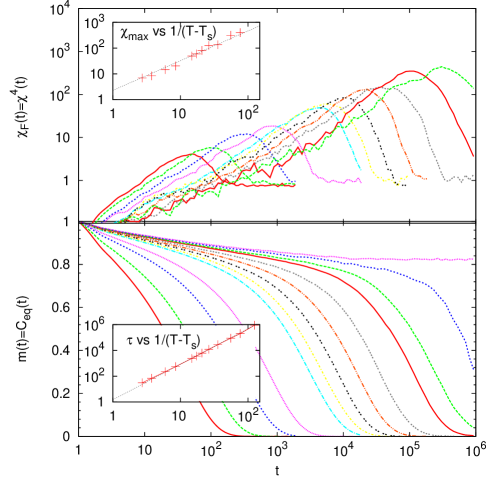
Figure 2: Dynamic ferromagnetic susceptibility and decay of the magnetization $m(t)$ in the melting on the Nishimori line for the $3$-spin model on the Bethe lattice with $c=5$ and $N=90000$ spins, averaged over $500$ realizations of the dynamics except for the three lower temperature where we used only $50$ runs. From left to right: $T=1.3$, $1.2$, $1.1$, $1.05$, $1.0$, $0.99$, $0.98$, $0.97$, $0.96$, $0.955$ and $0.95$. Bottom inset: the melting time [defined by $m(\tau)=1/e$] that diverges as a power law (35). Top inset: The maximum of the ferromagnetic susceptibility $\chi_{F}$ diverges as (36). The plotted quantities are identical to the dynamical susceptibility $\chi_{4}(t)$, eq. (33), and the equilibrium autocorrelation $C(t)$, eq. (32), in the spin glass phase.

Let us stress that this simulation would take a much longer time without the above trick that gives us an equilibrium configuration for free. Moreover, the method extends to temperatures $T_{K}\leq T\leq T_{\rm MCT}$ where Monte-Carlo equilibration takes an exponential time and is hence infeasible for such large system sizes.

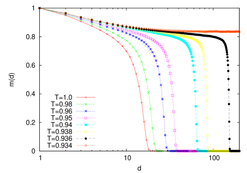
Figure 3: Magnetization at distance $d$ from a ferromagnetic boundary conditions in $3$-spin model on a Bethe lattice of coordination $c=5$ on the Nishimori line. This is the point-to-set correlation in the spin glass case. The correlation length diverges with exponent $1/2$ at $T_{\rm MCT}=0.936$.

The above mapping also allows to understand the point-to-set correlations DynamicBethe ; PointToSet in a simpler way. Point-to-set correlations are defined as follows: freeze the system in an equilibrium configuration. Then consider a large compact droplet in the system and un-freeze it to observe the influence of the frozen boundaries. For each temperature, one defines the equilibrium point-to-set volume as the largest size of the droplet such that the boundaries are correlated with the center of the droplet. Using the above mapping, this notion translates to a much simpler, and more easy to simulate, one: we just have to consider a system with fully ferromagnetic boundary conditions and ask if the magnetization stays positive in a center of a droplet of a certain size: This is the very same question we addressed in the purely ferromagnetic system in US-PART-I .

Point-to-set correlations in the mean-field spin glass case can be derived analytically and obey a simple solvable recursion (see DynamicBethe ). Our mapping shows (as can also be seen explicitly in the equations) that this recursion is identical to the one describing the way the magnetization decays at distance $d$ from ferromagnetic boundary conditions on the Nishimori line. We plot the solution to these equations in Fig. 3. Actually since the equations in question are very similar to what happens in pure ferromagnets, it is not surprising that the decorrelation length grows when $T_{\rm MCT}$ is approached with the exponent $1/2$ that was first obtained, for this model, in DynamicBethe .

III Glassy dynamics as a melting process in a finite dimensional model

We now discuss how is this mean field picture modified in finite dimensional systems. Since we are dealing with a glass transition, we should in principle use the mosaic theory, which is the counter-part of nucleation theory for glasses AdamGibbs ; KW1 ; KW2 ; KTW ; BiroliBouchaud . The fundamental point in this work is that due to the mapping to melting above a first order phase transition (from a ferromagnetic phase to a paramagnetic one) it is sufficient to consider the standard nucleation theory. This is a great conceptual simplification with respect to the many studied lattice models of glass formers Plaquette_L ; Plaquette_B ; STAR_model .

III.1 Nucleation theory for the melting of a disordered magnet

Let us very briefly recall the basics of nucleation theory, and discuss the effect of disorder for an entropy-driven first order phase transition. Nucleation stems from a competition between the bulk entropy difference and the surface tension between two phases. When a system is in a metastable phase the total free-energy cost $\Delta F(\ell)$ of a compact droplet of size $\ell$ is given by a combination of the bulk entropy $-\ell^{d}T\delta s$ and the surface tension $\ell^{\theta}\Gamma$, where $\delta s$ is the entropic difference between the two phases, $\theta\leq d-1$ is an exponent characterizing the free energy cost of the surface, and $\Gamma$ is the surface tension (we omit constant pre-factors for convenience). In a non-disordered systems we have $\theta=d-1$, but when disorder is present the shape of the droplet can adapt in order to take advantage of the local configuration of the disorder, so for the best droplet of each size we have $\theta\leq d-1$. The two contributions balance when the droplet size is

$$\ell_{\rm c}\propto{\left(\frac{\Gamma}{T\delta s}\right)}^{\frac{1}{d-\theta}}\propto(T-T_{c})^{-\nu}$$ (37)

with $\nu=1/({d-\theta})$, where we assumed that the difference $\delta s$ is linear when approaching the first order phase transition. For sizes larger than $\ell_{c}$ flipping a droplet is advantageous for the system. In order to flip, the thermal fluctuations must cross the free energetic barrier. In a non-disordered system one would expect that the barriers grow as $\ell_{c}^{\theta}$. However, this is only the free energy of the best droplet along the way, but the path that the dynamics is following is not bound to pass through this best droplet; it might actually have to go through larger barriers, and it is thus safer to assume instead that the barriers grow as $\ell^{\psi}$ with $\psi\geq\theta$. Using the Arrhenius formula we thus obtain the nucleation time

$$\tau\propto\exp\left[\frac{A}{T(T\delta s)^{\gamma}}\right]=\exp\left[\frac{\tilde{A}}{(T-T_{c})^{\gamma}}\right]$$ (38)

with $\gamma=\psi/{(d-\theta)}$.

So far we have, however, neglected an important ingredient: disorder induced fluctuations. We shall now present a scaling analysis in order to estimates the effect of the disorder on a first-order transition. Consider a droplet of size $\ell$, we expect that it can gain a free energy of order $\Delta F_{\rm dis}=\delta J\ell^{d/2}$ just from fluctuations in the free energy due to the disorder variance $\delta J$. The point is that this might be enough to make the droplet flip if the disorder induced term is larger than the surface term $\Gamma\ell^{\theta}$. Indeed, if $\theta<d/2$ there is a finite length $\xi_{\rm dis}\propto\left({{\Gamma}/{\delta J}}\right)^{1/(d/2-\theta)}$ beyond which the droplet flips independently of temperature. Hence in such a case the critical droplet size (that is, the point-to-set size) does not diverge at the transition point, and consequently the transition cannot be of first order. If we want a genuine first order phase transition, we thus must have $\theta\geq d/2$, or equivalently

$$\nu=1/{(d-\theta)}\geq 2/d.$$ (39)

For instance, the introduction of small amount of disorder in the pure ferromagnetic model, where $\theta=d-1$, cannot lead to a first order phase transition for $d<2$. The situation is the same in the marginal case $d=2$, as proven rigorously by Aizenmann and Wehr Self-3 . According to this analysis, we thus need at least a three-dimensional model if we want to have a hope for a genuine first order phase transition in the presence of disorder.

Finally, following the discussion from a companion paper US-PART-I , let us emphasize that the relevant mechanism for melting is nucleation and growth. The nucleation time $\tau$ (38) only gives the average time needed to nucleate a critical droplet at a given position in the system. If the system is much larger than the critical nucleus size the melting process is not done via the growth of a single droplet but instead results from the nucleation of many droplets that will simultaneously grow and invade the system. This growth time has to be added to the nucleation time to obtain the relaxation time needed to exit from the metastable state in a very large system. The probability to nucleate a critical droplet by a unit of volume and time is proportional to $e^{-\beta\Delta F(l_{c})}\propto 1/\tau$. Hence in a very large system there is roughly one droplet per volume $\tau$ after a unit of time. Without disorder, the volume of large droplets is expected to grow algebraically with time and consequently in the systems without disorder the total relaxation time is of the same order as the nucleation time $\tau$, and the typical size of grown droplets when they percolate is also scaling as $\tau$. This can be observed by looking to the dynamical ferromagnetic susceptibility, defined in eq. (25), as we have discussed in detail in US-PART-I for the Potts model. Clearly, the moment when such droplets percolate denotes the moment when the system is most heterogeneous, where roughly half of it is in the liquid phase and the other part still in the ordered one, so that the two-point dynamical ferromagnetic susceptibility is maximal.

Disorder will modify the growth behavior. Instead of the algebraic nucleus growth we expect instead an activated growth due to pining of the interfaces, just like in the coarsening of disordered magnets where the growth is logarithmic in time RFIM-th . The interplay between activated growth and the appearance of new droplets makes the total analysis more involved than in the case without disorder, and is a subject worthy of closer inspection in order to understand the melting of a crystalline ordered phase in presence of disorder. If the growth is slow, the melting will have to wait until many droplets have nucleated everywhere. Again, this gives a time of order $\tau$ for the melting process, but when droplets percolate, they are typically much smaller than in the non-disordered case. We will see that the dynamical magnetic susceptibility is again a suitable tool to quantify this understanding.

III.2 Nucleation vs mosaic on the Nishimori line

We now focus on a first order phase transition on the Nishimori line. Since we are discussing an entropy driven transition in a system with disorder, the analysis of the former paragraph applies. On the Nishimori line, however, the melting process is equivalent to the equilibrium dynamics. That means the system that is in a given equilibrium configuration decorrelates from this configuration by the nucleation mechanism to reach another equilibrium configuration which again will be left by activated nucleation and so on. Such a stationary melting process, where one transits from one equilibrium configuration to another by nucleation is nothing else than the phenomenology of the RFOT and the mosaic picture. Due to our mapping, however, it simply appears as a consequence of standard nucleation arguments.

For instance, eq. (38) is nothing but the Adam-Gibbs relation AdamGibbs ; KW1 ; KW2 ; KTW ; BiroliBouchaud , while eq. (37) is the mosaic length. The entropy difference is now associated with the number of metastable state so that $\delta s=\Sigma$ (where $\Sigma$ is the configurational entropy). According to the condition (39), we need $\nu\geq 2/d$, a conclusion was also reached in the seminal article on the RFOT KTW where in fact it was even argued that $\nu=2/d$, which combined with $\psi=\theta$ gives $\gamma=1$, which gives the original Adam-Gibbs relation. If indeed $\nu=2/d$ it suggests that if there is a first-order transition on the Nishimori line, it is a marginally stable one with respect to the smoothing by disorder. These questions, and in particular whether indeed $\nu=2/d$ or not, deserve further investigations.

An interesting (and hopefully clarifying) relation in our mapping is given by eq. (I.2). The four-point dynamical susceptibility $\chi_{4}(t)$, that describes the heterogeneous glassy dynamics, is simply the dynamical ferromagnetic susceptibility in the melting process. $\chi_{4}(t)$ thus acquires a simpler interpretation, as discussed in section III.1. The mapping on the Nishimori line thus allows to discuss the dynamics of glass forming liquids as a much simpler melting process. Let us illustrate this in a three-dimensional model.

III.3 A finite dimensional $p$-spin model

There are many ways how to introduce a $p$-spin model on a finite dimensional lattice (see for instance P-SPIN-FINITE ). We will use the following model on a three-dimensional cubic grid with each spin being involved in $10$ different $5$-body interactions

$${\cal H}= - \sum_{i}J^{a}_{i}S_{i}S_{\rm up}S_{\rm left}S_{\rm right}S_{\rm back}$$ (40)

$$- \sum_{i}J^{b}_{i}S_{i}S_{\rm down}S_{\rm left}S_{\rm right}S_{\rm front}\,,$$

where the indexes indicate the position of the spin on the grid with respect to the spin $i$. In the mean field case —that is on a Bethe lattice with $p=5$ and $c=10$— this model can be solved using the cavity method and it has qualitatively the phase diagram from Fig. 1, with a first order phase transition at $T_{c}(\rho=1)=2.4$ in pure case while on the Nishimori line, $e^{2\beta}=\rho/(1-\rho)$, we have $T_{c}(\rho_{\rm NL})=0.96$.

III.4 Numerical results

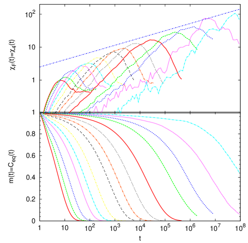
Figure 4: The dynamics on the Nishimori line for the $3$-dimensional $5$-spin model. Top: Dynamical susceptibility or equivalently the 4-point correlation function, $\chi_{4}(t)=\chi_{F}(t)$, as a function of time. Bottom: The magnetization or equivalently the equilibrium autocorrelation function, $C(t)=m(t)$, as a function of time. We use $1000$ realizations of the dynamics, except for the two lowest temperatures where we used only $50$ realizations. From left to right: $T=2.2$, $2.0$, $1.8$, $1.6$, $1.5$, $1.4$, $1.3$, $1.25$, $1.2$, $1.15$, $1.1$, $1.075$, $1.05$ and $T=1.025$. The peak of the dynamical susceptibility seems to increase slower than a power law of the relaxation time $\tau$. We show a power-law line with exponent $0.22$, which is the best power-law estimate for the largest time; however such a low value, and the general trend of the maxima, suggest that asymptotically the growth is logarithmic in $\tau$ (and thus algebraic in $T-T_{c}$) as expected for an actived coarsenning.

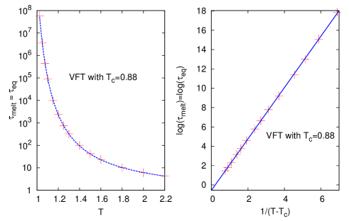
Figure 5: Melting time or equivalently the relaxation time $\tau$, in the $3$-dimensional $5$-spin model as a function of the temperature $T$ (plotted in a log-linear way on the left, and logarithm of the time versus $1/(T-T_{c})$ on the right). The dependence is very well fitted with a Vogel-Fulcher-Talman form $\tau\propto e^{\frac{A}{(T-T_{c})}}$, with $T_{c}\approx 0.88$.

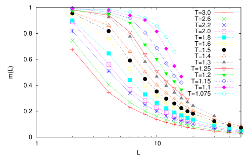
Figure 6: Point-to-set correlation, or equivalently equilibrium magnetization $m(T,L)$ in a box of size $L^{3}$ with ordered boundary conditions, for different temperatures. A clear sign a growing length scale as the temperature is lowered is observed.

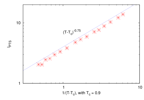
Figure 7: Point-to-set correlation length, defined as the size of the box where the magnetization in Fig. 6 goes below $2/3$. It is well fitted by $1/(T-T_{c})^{\nu}$ with $\nu \approx 0.75$ and $T_{c}=0.9$. Using instead the $1/[T(T-T_{c})]^{\nu}$ from (38) gives $\nu\approx 0.67$.

We now present results of numerical simulations of Hamiltonian (40) on the three-dimensional cubic grid on the Nishimori line. Studying the equilibrium dynamics on the Nishimori line, using the results of section I, is quite simple. We simulate the melting process starting from the fully ordered configuration, just as we did in the mean field system. Of course now the system on the Nishimori line is not equivalent anymore to the spin glass case with $\rho=1/2$, but this is irrelevant for our discussion. If there is a first order phase transition on the Nishimori line, then the melting process with a Vogel-Fulcher-Talman-like relaxation time and diverging length scales implies that the equilibrium dynamics undergoes an ideal glass transition described by the RFOT.

The correlation function for equilibrium dynamics (or equivalently the magnetization in the melting process) is plotted versus temperature in Fig. 4. It yields the standard picture with a growing plateau and the melting time —or equivalently the equilibrium auto-correlation time— grows faster than exponentially, and is perfectly consistent with a VFT divergence at $T_{c}=0.88$, as attested in Fig. 5. Note that we use the usual form of the VFT, but we could have used the generalized form eq. (38) with similar agreement but with slightly different values of $T_{c}$.

The upper part of Fig. 4 shows the dynamical susceptibility or equivalently the 4-point dynamical susceptibility. Its maximum $\chi_{4}^{\rm max}$ is growing with the growing relaxation time $\tau$. In US-PART-I we observed for the ferromagnetic two-dimensional non-disordered case that $\chi_{4}^{\rm max}\approx\tau$. The present data for the $5$-spin model on the Nishimori line instead indicate a low-exponent power law; in fact for the largest time the best power-law fit gives $\chi_{4}^{\rm max}\approx\tau^{0.2}$. Such a low exponent is compatible with a logarithmic growth in time; in fact a similar behavior is observed in the activated coarsening of the random field Ising model and in the random bond Ising model, where a logarithmic growth is expected RFIM-th but in numerical simulations a power-law with low exponent is observed RFIM-num . The low-exponent power law is in this case usually attributed to pre-asymptotic effects. The slower divergence of $\chi_{4}^{\rm max}$ in the presence of disorder (to be compared with the non-disordered transition in the Potts model observed in US-PART-I ) is thus due to an activated coarsening for the growth of the nuclei, as expected.

We also investigated the point-to-set correlation function PTS-Exp-Num . We consider a box of size $N=L^{3}$, apply fully ferromagnetic boundary conditions, and measure the equilibrium magnetization inside the box for different temperatures and sizes. Again, since we are on the Nishimori line, this is nothing but the point-to-set equilibrium correlation length, computed in a much faster way. The data are plotted in Fig. 6 and the correlation length in Fig. 7. We observe a growing length scale compatible with a power law divergence at $T_{c}$. By fitting our data using the formula $\ell\propto[T(T-T_{c})]^{-{\nu}}$ of eq. (37) we found that $T_{c}$ is compatible with the value $0.88$, and that the exponent $\nu$ is compatible with the value $2/3$ advocated in KTW .

Given we barely span two decades in Fig.7 one cannot be truly conclusive. Still, all our numerical results for the $5$-spin model on the 3-dimensional grid on the Nishimori line support the existence of a first order transition close to $T_{c}\approx 0.9$. Since the melting process is equivalent to equilibrium dynamics on the Nishimori line, this is a perfect realization of RFOT ideas in a finite dimensional setting. Below the Kauzmann transition the equilibrium physics is, however, given by the ferromagnetic phase, not by an ideal glass phase. This is not a problem, as this is after all what happens in real systems —the crystal is always the correct equilibrium state— and as we are mainly interested in how a liquid becomes a glass, not in the out-of-reach glass state below $T_{K}$ (which is anyway ill-defined STAR_model ).

III.5 Is there really a first order transition?

The numerical data are compatible with the existence of a first order phase transition on the Nishimori line, and as a consequence, with the existence of the ideal glass transition in a finite dimensional system. But is it really a genuine first order phase transition? Of course, this cannot be answered based only on numerical simulations, and we cannot exclude that if one goes to much larger times and to point-to-set lengths equal to, say, $\xi\approx 100$ a crossover to a second-order transition arises. Or worse, there might be no phase transition at all. Note, however, that such first-order transitions definitely exist at the mean field level (see section II.2) and that at least second-order ones do exist on the Nishimori line (see Jesper ) in finite dimension: We are thus assured that a transition can be found. At least, the issues and criticisms discussed in Moore , where it was argued that the RFOT transition in finite dimension maps only to a spin glass droplet model in a field, where it seems there is no transition at all Katz , do not apply in our case. The difficulty here is, however, to decide if on the Nishimori line there can be a first order phase transition in finite dimension.

Unfortunately, in all the solvable cases we found in the literature the transition on the Nishimori line is of the second order, e.g. Jesper . This is not very surprising because all these cases concern either 2-dimensional systems to which the theorem of Aizenman-Wehr Self-3 about smoothening of first order phase transition in the presence of disorder applies, either system which have a 2nd order phase transition even in the absence of disorder. If a genuine first order transition can be found on the Nishimori line in a 3D system is hence a challenging open question, which is clearly worth investigating.

Proving the existence or impossibility of a first order phase transition in a finite dimensional model on the Nishimori line would be a nice achievement. A positive answer would prove that a true VFT divergence exists in finite dimension, and that it is associated with a RFOT mechanism. However, on the practical side, this is not such a fundamental issue. If the transition becomes of 2nd order at sizes so large that the equilibrium behavior cannot be observed in a time smaller than any experimental time, then the first order approach for the melting problem (and the RFOT one for the glassy dynamics) is the correct description at the observable times scales.

IV Discussion

In this paper we have further studied the analogies between the melting dynamics above a first order phase transition and the equilibrium glassy dynamics discussed in US-PART-I by exploring a class of models where the two processes are strictly equivalent: Ising spin systems on the Nishimori line (some disordered Potts models share the properties discussed in this paper Jesper ). In the light of the mapping between melting and equilibrium dynamics, we investigated several features of the dynamics of super-cooled liquids: the diverging relaxation time, the plateau in the correlation function, dynamical heterogeneities related to the dynamical susceptibility $\chi_{4}$, and the point-to-set correlations. We show that they all can be easily recovered, understood, and studied in the much simpler, and more familiar, setting of first order phase transition. Since the RFOT was invented in analogy with first order transitions, it is rather interesting that there exist systems where the two are equivalent.

In particular, on the Nishimori line, the dynamical —or mode-coupling— transition corresponds to the spinodal point, while the Kauzmann transition corresponds to the first order ferromagnetic transition. The mosaic approach is replaced by simpler nucleation arguments. We hope this approach will help in expanding our comprehension of the glass transition problem. To conclude this work, we would like to make several comments.

Ideal glass transition?

A very fundamental open question in the field of glassy systems is the existence of a finite dimensional model where one can observe the VFT divergence. The bottom-line of our result here is that if there is a first order phase transition on the Nishimori line then the ideal glass transition exists. It would be very interesting to prove (or disprove) the existence of such a transition on the Nishimori line. Hopefully, this will be easier than the original question, as on the Nishimori line we are discussing a simpler to study first order phase transition. Moreover, the gauge transformation can be used to prove many results rigorously Nishimori .

String-like motion

It is well known in the theory of nucleation and first order phase transitions that the nucleating droplets can also be non-compact and fractal ReviewBinder . As noted by Wolynes , the stringy nuclei observed close to the pseudo-spinodal KLEIN in first-order transitions could be the analog of the string-like motion observed in the relaxation in glassy systems Sharon . The results presented here and the exact analogy between melting and glasses thus provide a firmer motivation for this. It would also be interesting to observe the string-like motion during the melting process of superheated solids: This is maybe related to the rings and loops observed in bulk melting simulations MO .

Mode coupling transition as a mean field approach

Many theoretical results about glasses are based on the mode coupling theory MCT ; MCT2 . The MCT predictions are exact in the mean-field $p$-spin model, and in this model the mode coupling transition can be mapped to a spinodal point of a first order phase transition on the Nishimori line. One hence cannot escape the conclusion that the transition described by MCT is a kind of mean-field melting, and the mode coupling temperature is a corresponding spinodal point. Of course, this suggestion is present in the literature since the work of KT ; KW1 ; KW2 , but our mapping makes it very explicit.

Simulating MCT behavior

A straightforward but powerful application of our mapping is to perform fast simulations of the equilibrium glassy dynamics in mean-field models, as we have done for the $p$-spin, by simply starting from the fully ordered configuration. This should allow us to go beyond the current size limitations and investigate better numerically the mean-field systems and the finite-size corrections (in the spirit of e.g. SarlatBilloire09 ). This is in fact what we have started to do in section II.3.

Crossover MCT/finite dimension

One of the crucial issues in the RFOT is to understand better nucleations in glassy systems, and our mapping allows to put this question back into the standard framework of first order phase transitions. The crossover from the mode coupling behavior to the finite dimensional activated dynamics (described e.g. by the mosaic theory) then becomes the usual crossover from spinodal to activation at a first order phase transition ReviewBinder . A promising direction in which these ideas could be extended is the Kac limit SILVIO , or the field theoretic computation of instanton in order to estimate the free energetic barriers. Note also that the system is guarantied to be replica symmetric on the Nishimori line which may simplify many calculations.

- (1) P. G. Debenedetti and F. H Stillinger, Nature 410, 6825 pp. 259-267 (2001).
- (2) M. D. Ediger, C. A. Angell, S. R. Nagel, J. Phys. Chem. 100, 13200 (1996).
- (3) C. A. Angell, Journal of Physics and Chemistry of Solids 49, n. 8, 863-871 (1988).
- (4) H. Vogel, Phys. Z. 22, 645 (1921). G. S. Fulcher, J. Am. Ceram. Soc. 8, 339 (1925).
- (5) W. Kauzmann, Chem. Rev., 43 (2), 219 (1948).
- (6) G. Adam, J. H. Gibbs, J. Chem. Phys. 43, 139–146 (1965).
- (7) S. Franz and G. Parisi, J. Phys.: Condens. Matter 12, 6335 (2000).
- (8) C. Toninelli et al., Phys. Rev. E 71, 041505 (2005).
- (9) E. R. Weeks et al., Science 287, 627-631 (2000).
- (10) J.-P. Bouchaud and G. Biroli, J. Chem. Phys. 121, 7347–7354 (2004).
- (11) A. Montanari and G. Semerjian, J. Stat. Phys. 124, 103 (2006).
- (12) A. Montanari and G. Semerjian, J. Stat. Phys. 125, 23 (2006).
- (13) A. Cavagna, T. S. Grigera and P. Verrocchio, Phys. Rev. Lett. 98, 187801 (2007). G. Biroli, J.-P. Bouchaud, A. Cavagna, T. S. Grigera and P. Verrocchio, Nature Physics 4, 771 (2008).
- (14) T. R. Kirkpatrick and D. Thirumalai, Phys. Rev. Lett. 58, 2091 (1987). T. R. Kirkpatrick and D. Thirumalai, Phys. Rev. B 36, 5388 (1987).
- (15) T. R. Kirkpatrick and P. G. Wolynes, Phys. Rev. A 35 3072 (1987).
- (16) T. R. Kirkpatrick and P. G. Wolynes, Phys. Rev. B 36 8552 (1987).
- (17) T. R. Kirkpatrick, D. Thirumalai, P. G. Wolynes, Phys. Rev. A 40, 1045–1054 (1989).
- (18) M. Mézard and G. Parisi, Phys. Rev. Lett. 82, 747 (1999).
- (19) J.S. Langer, Phys. Today 8–9 (2007).
- (20) G. Biroli and J.-P Bouchaud, arXiv:0912.2542 (2009).
- (21) F. Krzakala and L. Zdeborová, Glassy aspetcs of melting dynamics, in preparation.
- (22) B. Derrida, Phys. Rev. Lett. 45, 79 - 82 (1980). B. Derrida, Phys. Rev. B 24, 2613 - 2626 (1981).
- (23) D. J. Gross and M. Mézard, Nucl. Phys. B 240, 431 (1984).
- (24) F. Ricci-Tersenghi, M. Weigt and R. Zecchina, Phys. Rev. E 63, 026702 (2001). S. Franz et. al. Europhys. Lett. 55, 465-471 (2001).
- (25) H. Nishimori, Prog. Theor. Phys. 66, 1169 (1981).
- (26) H. Nishimori, Statistical Physics of Spin Glasses and Information Processing: An Introduction (Oxford, 2001).
- (27) Y. Ozeki, J. Phys. A: Math. Gen. 28, 3645 (1995).
- (28) Y. Ozeki, J. Phys.: Condens. Matter 9, 11171 (1997).
- (29) S. F. Edwards and P. W. Anderson 1975 J. Phys. F: Met. Phys. 5 965
- (30) M. Mézard, G. Parisi, and M. A. Virasoro, Spin-Glass Theory and Beyond, Lecture Notes in Physics Vol. 9 (World Scientific, Singapore, 1987).
- (31) J. Hertz and K. H. Fischer, Spin Glasses (Cambridge Universtity Press, 1991).
- (32) M. Goldstein, J. Chem. Phys. 51, 3728 (1969).
- (33) A. Lipowski, and D. Johnston, Phys. Rev. E 64, 041605 (2001)
- (34) M. R. Swift, H. Bokil, R. D. M. Travasso and A. J. Bray, Phys. Rev. B 62, 11494–11498 (2000).
- (35) A. Cavagna, I. Giardina and T. S. Grigera J. Chem. Phys. 118, 6974 (2003).
- (36) A. Georges, D. Hansel, P. Le Doussal and J-M Maillard, J. Phys. 48, 1 (1987). Y. Kasai and A Okiji, Prog. Theor. Phys. 69, 20 (1983).
- (37) S. Franz and M. Leone, J. Stat. Phys. 111, 535 (20903).
- (38) F. Guerra and F. L. Toninelli, Commun. Math. Phys. 230, 71–79 (2002).
- (39) J. Wehr and M. Aizenman, J. Stat. Phys. 60, 287 (1990). M. Aizenman and J. Wehr, Phys. Rev. Lett. 62, 2503–2506 (1989)
- (40) S. Franz, G. Parisi, Phys. Rev. Lett. 79, 2486 (1997).
- (41) S. Franz et al., arXiv:1001.1746 and arXiv:1008.0996.
- (42) K. Binder, Rep. Prog. Phys. 50 783-859 (1987).
- (43) K. Binder, Phys. Rev. B 8, 3423–3438 (1973).
- (44) W. G. Hoover and F. H. Ree, J. Chem. Phys. 49, 3609 (1968).
- (45) D. Frenkel, Physica A 263 26 (1999).
- (46) F. Krzakala and L. Zdeborová, arXiv:0909.3820, to appear in EPL (2010).
- (47) L. Zdeborová and F. Krzakala, Phys. Rev. B 81, 224205 (2010).
- (48) L. Cugliandolo and J. Kurchan, Phys. Rev. Lett. 71, 173 (1993).
- (49) J.-P. Bouchaud et al., Physica A 226 243 (1996). J.-P. Bouchaud et al., in Spin Glasses and Random Fields, edited by A. P. Young (World Scientific, Singapore, 1998).
- (50) A. Cavagna, I. Giardina and G. Parisi, J. Phys. A: Math. Gen. 34 5317-5326 (2001).
- (51) D. Achlioptas and A. Coja-Oghlan, arXiv:0803.2122 (2008).
- (52) L Zdeborová and F. Krzakala, arXiv:0902.4185v1 (2009).
- (53) F. Krzakala and L Zdeborová, Phys. Rev. Lett. 102, 238701 (2009).
- (54) S. Franz, G. Parisi, Physica A 261, 317 (1998).
- (55) P. Gillin, H. Nishimori and D. Sherrington, J. Phys. A: Math. Gen. 34 2949 (2001).
- (56) H. Nishimori and K. Y. M. Wong, Phys. Rev. E 60, 132 (1999).
- (57) W Gotze, J. Phys.: Condens. Matter 2 SA201 (1990),
- (58) S. P. Das, Rev. Mod. Phys. 76, 785 (2004).
- (59) G. Biroli and J.-P. Bouchaud, Europhys. Lett. 67, 21 (2004).
- (60) D. A. Huse and C. L. Henley, Phys. Rev. Lett. 54 (1985), 2708. D.S. Fisher, D.A. Huse Phys. Rev. B 38 373 (1988).
- (61) D. Alvarez, S. Franz, F. Ritort, Phys. Rev. B 54, 9756(1996). H. Rieger, Physica A 184, 279 (1992), J. Kisker, H. Rieger, H. Schreckenberg, J. Phys. A 27, L853 (1994). S. Franz and G. Parisi, Eur. Phys. J. B 8, 417–422 (1999).
- (62) R. Paul, S. Puri, and H. Rieger, Europhys. Lett. 68, 881 (2004). H. Rieger, G. Schehr, R. Paul, Prog. Theor. Phys. Suppl. 157, 111 (2005)
- (63) J. Jacobsen and M. Picco, Phys. Rev. E 65, 026113 (2002).
- (64) M. A. Moore and B. Drossel, Phys. Rev. Lett. 89, 217202 (2002).
- (65) T. Jörg, H. G. Katzgraber and F. Krzakala, Phys. Rev. Lett. 100, 197202 (2008) .
- (66) J. D. Stevenson, J. Schmalian and P. G. Wolynes, Nature Physics 2, 268-274 (2006).
- (67) H. Wang, H. Gould and W. Klein, Phys. Rev E 76, 031604 (2007)
- (68) C. Donati et al, Phys. Rev. Lett. 80, 2338–2341 (1998).
- (69) X-M Bai and M. Li, Phys. Rev. B 77, 134109 (2008).
- (70) T. Sarlat et al., J. Stat. Mech. P08014 (2009).
- (71) S. Franz and F. L. Toninelli, Phys. Rev. Lett. 92, 030602 (2004). S. Franz et al. J. Phys. A: Math. Theor. 40 F251-F257 (2007).