Exploring the randomness of Directed Acyclic Networks

Abstract

The feed-forward relationship naturally observed in time-dependent processes and in a diverse number of real systems -such as some food-webs and electronic and neural wiring- can be described in terms of so-called directed acyclic graphs (DAGs). An important ingredient of the analysis of such networks is a proper comparison of their observed architecture against an ensemble of randomized graphs, thereby quantifying the randomness of the real systems with respect to suitable null models. This approximation is particularly relevant when the finite size and/or large connectivity of real systems make inadequate a comparison with the predictions obtained from the so-called configuration model. In this paper we analyze four methods of DAG randomization as defined by the desired combination of topological invariants (directed and undirected degree sequence and component distributions) aimed to be preserved. A highly ordered DAG, called snake-graph and a Erd os-Rényi DAG were used to validate the performance of the algorithms. Finally, three real case studies, namely, the C. elegans cell lineage network, a PhD student-advisor network and the Milgram’s citation network were analyzed using each randomization method. Results show how the interpretation of degree-degree relations in DAGs respect to their randomized ensembles depend on the topological invariants imposed. In general, real DAGs provide disordered values, lower than the expected by chance when the directedness of the links is not preserved in the randomization process. Conversely, if the direction of the links is conserved throughout the randomization process, disorder indicators are close to the obtained from the null-model ensemble, although some deviations are observed.

I Introduction

Many relevant properties of complex systems can be described by an appropriate network representation of their elements and interactions Watts and Strogatz (1998); Newman et al. (2001); Dorogovtsev and Mendes (2003); Sole et al. (2003); Boccaletti et al. (2006). Most of these networks are directed, i. e. there is a directional relationship between two elements defining who influences who in a given order. Among the class of directed networks, directed acyclic graphs -henceforth, DAGs- are an important subset lacking feedback loops. This is specially suitable for the representation of evolutionary, developmental and historical processes in which the time asymmetry determines a feed-forward (acyclic) flow of causal relations. In this context, DAGs constitute a formal representation of causal relations that display the direct effects of earlier events over latter ones. Citation networks are among their most paradigmatic cases Hummon and Doreian (1989); E. et al. (1964). In these networks nodes are scientific articles and directed links (or arcs) stand for bibliographic citations among them. According to a chronological order, directed links are established from former articles to newer ones in a feed-forward manner.

In general, time-dependent processes have been formalized as DAGs. Examples of that comprehend article and patent citation networks Valverde et al. (2007); Csardi et al. (2007), decision jurisprudence processes Fowler and Jeon (2008); Chandler (2005) and tree genealogies and phylogenies. Moreover, other relevant systems such as standard electric circuits Clay (1971), feed-forward neural Haykin (1999) and transmission networks Frank and Frisch (1971) are also suitably represented as DAGs.

The main objective of this paper is to explore the randomness -in topological terms- of real systems displaying a directed acyclic structure by the defintion a collection of randomization methods that preserves a fixed number of topological invariants. To this end, the design of null models to highlight the particular features characterizing a system with respect to a neutral or random scenario Newman et al. (2001) is needed. In this context, the so-called configuration model Newman et al. (2001); Dorogovtsev and Mendes (2003); Fulton et al. (2001); Molloy and Reed (1995) has been probed as a fruitful approximation to provide a null-model scenario of what is expected by chance in complex networks under the assumptions of sparseness, infinite size and lack of correlations. However, little attention has been paid concerning DAGs. Indeed, a rigorous definition of random DAG from its directed degree sequence has been recently proposed Karrer and Newman (2009), rising the interest for its study through configuration model approach. Borrowing the methodology to build random undirected graphs Molloy and Reed (1995); Aiello et al. (2001), degree sequence is visualized as a set of edge stubs. Hence a random DAG is constructed by matching stubs according to certain order constraints until they are completely canceled Karrer and Newman (2009). Without neglecting the important advance it represents for the comprehension of acyclic networks, some problems arise in using this methodology as the null model reference of real nets. Firstly, this methodology is dependent on how probable is to construct a graph from a degree sequence, since not all of them produce a graph, i.e., they are not graphical. Additionally, configuration model assumptions are not fulfilled in real systems due to their finite size and the presence of densely connected regions.

An alternative approach used in this work is based on iterative processes of edge rewiring over the graph, keeping the graphical condition during all the process of randomization. This is a relevant issue since the degree sequence, either directed or undirected, imposes a particular space of topological configurations rather limited -as we shall see in this work- for DAGs. Attending to this approach we can estimate where a real graph is placed preserving a graphical ensemble that holds some topological invariants. The two fundamental topological invariants considered in this work for a null model comparison are the degree sequence (either directed or undirected) and the component structure. The both types of degree sequences and the degree distribution have been typically chosen as invariant in the random model construction Molloy and Reed (1995); Newman et al. (2001); Maslov and Sneppen (2002); Karrer and Newman (2009). However, as is well known in random graph theory, the existence of some graph satisfying a given degree sequence does not guarantee a single connected component containing the whole set of nodes, except at high connectivities. Therefore sparse networks representing connected systems are expected to be fragmented during a randomization process. This may be an undesirable effect when studying historical processes since it breaks the flow of causality. Besides this problem, there are also real systems that display more than a single connected component. Those disconnected components do not interact among them and, arguably, can be considered to be independent systems in terms of causality. It is worth to note that preservation of connected component in graph randomization processes has recently raised the interest of network community Han (2009).

According to the above considerations, in order to produce comparable ensembles for the evaluation of the randomness of a real DAG, we propose a collection of four randomization methods for DAGs that ensure the topological invariants mentioned above. These randomization techniques were applied to two extreme -in terms of degree-degree relations- network models: an Erdös Rényi DAG and a highly ordered graph called snake-DAG. Our methodology was then applied to three real DAGs: a citation network, a PhD-student advisor network and the cell lineage in the development of caebnorhabditis elegans worm.

The paper is organized as follows: Section II offers the basic concepts related to DAGs. Section III explicitly defines the set of four randomization algorithms according to different topological invariants. Section IV describes and characterizes the randomness indicators and apply the randomization processes to the systems under study: two toy models -which enable us to validate the performance of the algorithms- and three real systems. Section V discusses the relevance of the obtained results.

II Ordering, causality and formal definition of DAGs

In this section we discuss some mathematical properties of DAGs and their interpretation in terms of causal relations. We finally address the problem of component structure conservation.

II.1 Basic definitions

Let ${\cal G}(V,E)$ be a directed graph, being $V=\{v_{1},...,v_{N}\}$ the set of nodes, and the set of ordered pairs $E=\{\langle v_{k},v_{i}\rangle,...,\langle v_{j},v_{l}\rangle\}$ the set of edges -where the order, $\langle v_{k},v_{i}\rangle$ implies that there is an arrow in the following direction: $v_{k}\rightarrow v_{i}$. The underlying graph ${\cal G}_{u}$ of a directed graph ${\cal G}$ is an undirected graph with the same set of nodes ${\cal G}$, but whose edges are undirected (i.e. $\langle v_{k},v_{j}\rangle\in E$, then $\{\langle v_{j},v_{k}\rangle,\langle v_{k},v_{j}\rangle\}\in E_{u}$). Given a node $v_{i}\in V$, the number of outgoing links, to be noted $k_{o}(v_{i})$, is called the out-degree of $v_{i}$. Similarly, the number of ingoing links of $v_{i}$ is called in-degree of $v_{i}$, noted by $k_{i}(v_{i})$.

A DAG is a directed graph characterized by the absence of cycles: If there is a directed path from $v_{i}$ to $v_{k}$ (i.e., there is a finite sequence $\langle v_{i},v_{j}\rangle,\langle v_{j},v_{l}\rangle,\langle v_{l},v_{s}\rangle,...,\langle v_{m},v_{k}\rangle\in E$) then, there is no directed path from $v_{k}$ to $v_{i}$. Borrowing concepts from order theory Suppes (1960); Kelley (1955), we refer to nodes with $k_{i}=0$ as maximals and those with $k_{o}=0$ as minimals. The absence of cycles ensures that at least there is one minimal node and one maximal node. Maximal nodes can be seen as inputs of a given computational or sequential process while minimal -or terminal- ones are the outputs of such a process. Furthermore the acyclic nature permits to define a node ordering by labeling all nodes with sequential natural numbers. Thus, in a DAG there is at least one numbering of the nodes such that:

$$(\forall\langle v_{i},v_{j}\rangle\in E)\Rightarrow(i>j).$$ (1)

For this reason, DAGs have been also referred as ordered graphs Karrer and Newman (2009).

II.2 Random DAGs

The theoretical roots of the concept of a random DAG are based on the so-called directed degree sequence Karrer and Newman (2009) -as well as the concept of random graph Molloy and Reed (1995). A random DAG ${\cal G}$ is a randomly chosen element of an ensemble of DAGs which share the directed degree sequence, denoted by $d({\cal G})$, which is defined as follows:

$$d({\cal G})=(k_{i}(v_{1}),k_{o}(v_{1})),...,(k_{i}(v_{i}),k_{o}(v_{i})),...$$ (2)

The two numerical quantities composing every element of such a sequence, $k_{i}(v_{k})$ and $k_{o}(v_{k})$, encode the pattern of connectivity of every node of the graph. In general, the ensemble of random graphs containing $N$ nodes is composed by all possible graphs whose connectivity pattern satisfies the directed degree sequence. If we only pay attention to the number of edges connected to a given node $v_{i}$ -regardless the direction of the arrows- we define the degree of the node $v_{i}$ as $k(v_{i})=k_{i}(v_{i})+k_{o}(v_{i})$ and, consistently, the undirected degree sequence of ${\cal G}$, is defined as:

$$d_{u}({\cal G})=k(v_{1}),...,k(v_{i}),...$$ (3)

However, it is clear that not any sequence of $N$ pairs of natural numbers -or $N$ natural numbers in the case of the undirected degree sequence- represents the degree sequence of an ensemble of some kind of random graphs containing $N$ nodes Molloy and Reed (1995); Karrer and Newman (2009). There are several restrictions that a (un)-directed degree sequence must satisfy in order to represent a proper graph, i.e., a sequence to be graphical or feasible Molloy and Reed (1995). In the case of directed graphs, in and out degrees of the whole sequence must be consistent with the number of edges, i.e.:

$$\sum_{i\leq n}k_{i}(v_{i})=\sum_{i\leq n}k_{o}(v_{i})=|E|,$$ (4)

It is clear that such a condition does not avoid the presence of cycles in the network structure. Consistently with the claim that DAGs depict systems where some unavoidable ordering among nodes is at work, we can ensure the generation of a given DAG if and only if there is a labeling of the nodes such that $v_{i}\to v_{j}$ implies that $i>j$. Taking into account this ordering to build the graph, the directed degree sequence must also hold two conditions. First,

$$k_{o}(v_{1})=k_{i}(v_{n})=0,$$ (5)

and second,

$$(\forall v_{i}\in V)\;\;\sum_{j<i}k_{i}(v_{j})-\sum_{j\leq i}k_{o}(v_{j})\geq 0.$$ (6)

Under conditions (4,5,6) it is ensured that a directed degree sequence will be graphical and able to represent the degree sequence of a given non-empty ensemble of DAGs.

II.3 Component structure and causal relations

The concept of component structure stems from the notion of undirected path: given two pairs of nodes $v_{i},v_{k}\in V$, there is an undirected path among them if there is a finite sequence of undirected edges such that it can be ordered sequentially, for example $\{v_{i},v_{j}\},\{v_{j},v_{l}\},\{v_{l},v_{s}\},...,\{v_{m},v_{k}\}\in E_{u}$. A component of ${\cal G}$ is a (maximal) subset of $V$ by which an undirected path can be defined among any pair of nodes. The special features of a DAG impose constraints on the number of -DAG like- components from a given directed degree sequence. Indeed, let $M({\cal G})=\{v_{k}\in V:k_{i}(v_{k})=0\}$ be the set of maximal nodes of a given DAG ${\cal G}$ and $\mu({\cal G})=\{v_{k}\in V:k_{o}(v_{k})=0\}$ the set of its minimal nodes. Let $d({\cal G})$ be the directed degree sequence of ${\cal G}$ which, by assumption, is graphical. Then, the number of (DAG) components of the graph $c({\cal G})$ is bounded by

$$c({\cal G})\leq\min\{|M|,|\mu|\},$$ (7)

since any connected DAG must have, at least, $|\mu|=|M|=1$. Another constraint must be satisfied. There must exist a partition of the directed degree sequence $d({\cal G})$ by which all $c({\cal G})$ subsequences are graphical, i.e., they satisfy equations (4,5,6).

III Randomization Methods

This section describes four methods to obtain randomized ensambles of DAGs, preserving a number of invariants. The four algorithms presented below perform random rewirings according to constraints based on (un)-directed degree sequence and component structures, all of them explicitly avoiding the presence of multi-edges. Algorithms presented in this work are illustrated in figure 1. For the sake of clarity the order of presentation of the methods is the same for all figures and tables, and thus the letters used in fig. (1) inequivocaly identify the methods of randomization.

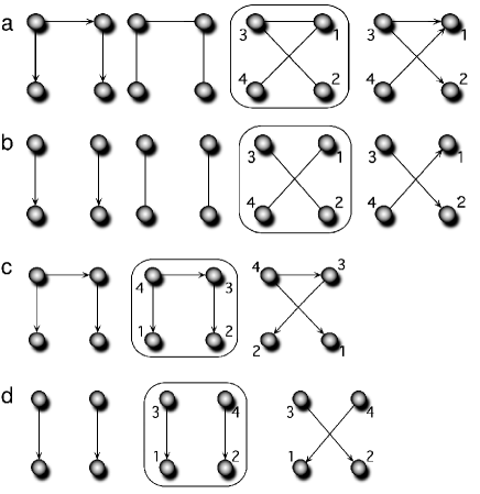
Figure 1: Schematic representation of the four different DAG randomizations proposed in this work. Methods are alphabetically denoted (a to d). Method $\mathbf{a}$: randomization preserving undirected degree sequence and component size distribution. Method $\mathbf{b}$: DAG randomization only preserving the undirected degree sequence. Method $\mathbf{c}$: randomization preserving directed degree sequence and component size distribution. Method $\mathbf{d}$: randomization preserving only directed degree sequence.

III.1 Generating the ensemble from the undirected degree sequence

The simplest method of randomization preserving components consists of applying a random numbering to ${\cal G}^{u}$. This allows us to define an order criteria to establish the direction of arrows. In this case, given an undirected pair $\{v_{i},v_{j}\}$ we say that if $i>j$ we defined the order pair as $\langle v_{j},v_{i}\rangle$, otherwise $\langle v_{i},v_{j}\rangle$. Since ${\cal G}^{u}$ is preserved, undirected degree-degree relations are also conserved. Then, a suitable randomization requires some additional process of link rewiring to destroy the presence of degree-degree relations. In this context, we provide a methodology that combines a rewiring process that preserves undirected degree sequence -see eq. (3)-, component structure and renumbering.

This first randomization method, denoted by the letter ${\mathbf{a}}$, is depicted in fig. (1a). The steps of the algorithm are scheduled in the following:

1. Given a DAG, ${\cal G}(V,E)$, we obtain its respective underlying network, ${\cal G}_{u}$.

2. We obtain a random network conserving the undirected degree sequence of ${\cal G}_{u}$ and its component structure by a randomization process denominated local-swap Han (2009). Local-swap is performed as follows: We randomly select an existing edge $\{v_{i},v_{j}\}$ of ${\cal G}_{u}$ such that the two additional edges $\{v_{i},v_{k}\}$ and $\{v_{j},v_{l}\}$ also exist in ${\cal G}_{u}$, provided that $v_{k},v_{i},v_{j},v_{l}$ are all different. Then we proceed to make the rewiring, by generating the edges $\{v_{i},v_{l}\}$ and $\{v_{j},v_{k}\}$; and removing the edges $\{v_{i},v_{k}\}$ and $\{v_{j},v_{l}\}$. If $\{v_{i},v_{l}\}$ or $\{v_{j},v_{k}\}$ already exist in ${\cal G}_{u}$ we abort the operation and we randomly select another edge satisfying the above described conditions to perform the local swap. According to Han (2009), local-swap method can perform all rewirings of links except those that imply the breaking of the component structure. This process is iteratively repeated until achieving a suitable randomization of ${\cal G}_{u}$ or after a predefined number of iterations.

3. Once the local-swap randomization of ${\cal G}_{u}$ is done, we label every node with an arbitrary natural number, from $1$ to $N$, being $N$ the size of the graph. No repetitions are allowed.

4. We now proceed to define the arrows taking into account the numbering of the nodes defined in the previous step. For every pair of connected nodes in the randomized version of ${\cal G}_{u}$, we define the arrow from lower to higher number’s nodes. Formally, given a undirected pair $\{v_{i},v_{j}\}$ where $i,j$ are the respective labels obtained through the random numbering, if $i>j$ then $v_{i}\to v_{j}$, otherwise $v_{i}\leftarrow v_{i}$. The total order of natural numbers avoids the presence of cycles.

Method ${\mathbf{b}}$ consists of preserving the undirected degree sequence but not preserving component structure. Component structure is ensured by step 2) in method ${\mathbf{a}}$. In this case, step 2) is replaced by a direct rewiring process: $i)$ selecting a pair of different edges $\{v_{i},v_{k}\},\{v_{j},v_{l}\}$ of ${\cal G}_{u}$; $ii)$ Generate with probability $p=1/2$ either the edges $\{v_{i},v_{l}\},\{v_{j},v_{k}\}$ or the edges $\{v_{i},v_{j}\},\{v_{l},v_{k}\}$ (provided that both two edges are not already present) and $iii)$ remove the edges $\{v_{i},v_{k}\},\{v_{j},v_{l}\}$ -see fig. (1b).

III.2 Generating the ensemble from the directed degree sequence

Beyond the randomization of the raw topological structure of the real DAG conserving component structure, one could be interested in the preservation of the directed degree sequence -see eq. (2). This has an important physical interpretation, since it implies that every node has an invariant number of inputs and outputs, as it happens with the components of an electronic device. Under such a restriction we can no longer work with the underlying graph but with the directed graph.

The proposed algorithm, denoted by method ${\mathbf{c}}$ -see fig. (1c)-, begins with a numbering of the nodes resulting from the application of a leaf-removal algorithm Rodriguez-Caso et al. (2009) and a rewiring operation constrained by this numbering. Let us briefly revise how a leaf-removal algorithm works: From the original graph, ${\cal G}$, we iteratively remove the nodes with $k_{o}=0$ until the complete pruning of the graph. According to this, a DAG can be layered, and thus a partial order between nodes can be easily established. Formally, the $i$-th iteration of the leaf-removal algorithm defines the set $V_{i}\subseteq V$ of nodes where $V_{i}$ corresponds the $i$-th layer of the DAG. Then, any DAG can be redefined in terms of the resulting -ordered- layers of a leaf-removal algorithm, i.e.,

$$W({\cal G})=\{W_{1},...,W_{l}\}$$ (8)

where no link between nodes of the same layer is established.

Method ${\mathbf{c}}$ -see fig. (1c)- is defined as follows:

1. Generate the set $W({\cal G})$ by applying the leaf removal algorithm.

2. Perform a random numbering of the nodes in such a way that, given $v_{i}\in W_{u}$, and $v_{k}\in W_{s}$,

   $$(u>s)\rightarrow(i>k)$$ (9)

3. Select at random an edge $\langle v_{k},v_{j}\rangle\in E$. Then we look for the presence of two nodes $v_{i}$, $v_{l}\in V$ by which either:

   $$i) \langle v_{i},v_{k}\rangle,\langle v_{l},v_{j}\rangle\in E,\;\;{\rm or}$$ (10)

   $$ii) \langle v_{k},v_{i}\rangle,\langle v_{j},v_{l}\rangle\in E.$$ (11)

   Notice that the absence of cycles makes these two options mutually exclusive.

4. If the condition (10) is satisfied, the pairs $\langle v_{l},v_{k}\rangle$ and $\langle v_{i},v_{j}\rangle$ are generated and $\langle v_{i},v_{k}\rangle$,$\langle v_{l},v_{j}\rangle$ deleted, provided that the following conditions are satisfied: 1)$\langle v_{l},v_{k}\rangle\langle v_{i},v_{j}\rangle\notin E$ and 2)$l>k$ and $i>j$. If one of these two conditions does not hold, the rewiring event is aborted and another edge is newly selected at random.

   If condition (11) is satisfied, the pairs $\langle v_{k},v_{l}\rangle$ and $\langle v_{j},v_{i}\rangle$ are generated, deleting $\langle v_{k},v_{i}$, $\rangle\langle v_{j},v_{l}\rangle$ links, provided that $\langle v_{k},v_{l}\rangle\langle v_{j},v_{i}\rangle\notin E$ and $k>l$ and $j>i$ conditions are satisfied. Again, if one of these two conditions does not hold the rewiring event is restarted.

Finally, the randomization method ${\mathbf{d}}$ preserves the directed degree sequence but do not preserve the component strucutre. In this case, step 3) is replaced by the following procedure: $i)$ select two edges at random $\langle v_{k},v_{i}\rangle,\langle v_{l},v_{j}\rangle\in E$; $ii)$ generate the edges $\langle v_{k},v_{j}\rangle,\langle v_{l},v_{i}\rangle$ provided that $\langle v_{k},v_{j}\rangle,\langle v_{l},v_{i}\rangle\notin E$ and that $k>j,l>i$. If some of these conditions does not hold, process is aborted and we restart the rewiring event. $iii)$ If conditions are satisfied, $\langle v_{k},v_{i}\rangle,\langle v_{l},v_{j}\rangle$ are removed -see fig. (1d).

IV Exploring the randomness of DAGs

In this section we apply the above defined algorithms to some real topologies to construct an ensemble of randomized networks (also known as surrogate data in other scientific communities) preserving the defined topological invariants. First of all, we need to define proper measures to evaluate the level of randomness of our systems.

IV.1 Testing the success of the randomization process

As it is described above, randomizations are subject to very restrictive constraints since not all (un)-directed degree sequence configurations are graphical. Therefore, the success of DAG randomization processes must be properly evaluated. Two estimators were measured for this purpose. First, a dissimilarity parameter ${\cal D}$ is proposed to measure how the graph evolves along the iterations with respect to the original one. Second, the deterioration of present degree-degree relations is also reported by means of an estimator borrowed from information theory, the so-called joint entropy Shannon (1948).

IV.1.1 Dissimilarity

The dissimilarity parameter ${\cal D}$ between two graphs is the relative frequency of link mismatches between them, i.e., the Hamming distance of their adjacency matrices. In the context of a randomization process, let us define ${\cal A}$ and ${\cal A}^{t}$ as the adjacency matrices of an original graph (${\cal G}$) and the graph resulting from the application of $t$ randomization iterations (${\cal G}^{t}$), respectively. Their dissimilarity can be expressed as

$${\cal D}({\cal G},{\cal G}^{t})\equiv\frac{1}{2|E|}\sum_{i,j}1-\delta({\cal A}_{ij},{\cal A}_{ij}^{t}),$$ (12)

where $\delta$ is the Kronecker’s delta and $|E|$ denotes the number of links of both ${\cal G}$ and ${\cal G}^{t}$, since the undirected degree sequence is preserved in the four randomization methods.

IV.1.2 Degree-degree joint entropy

Given two random variables, $X,Y$, the joint entropy between $X$ and $Y$, $H(X,Y)$ is given by:

$$H(X,Y)=-\sum_{x,y}\mathbb{P}(x,y)\log(\mathbb{P}(x,y),$$ (13)

being $\mathbb{P}(X,Y)$ the joint probability of the pair of outcomes $x,y$ happening together -throughout this paper $\log_{2}$ will be used. Let us detail how every concept is translated in a useful way to become graph measures.

Joint entropy for the evaluation of degree-degree relations can be expressed as

$$H({\cal G}_{u})=\sum_{i\geq j}\mathbb{P}(i,j)\log\mathbb{P}(i,j)$$ (14)

where $\mathbb{P}(i,j)$ defines the probability of finding a randomly selected link that connects two nodes $v_{m},v_{l}\in V$ such that $k(v_{m})=i,\;k(v_{l})=j$. This measurement was found to be more appropriate than other existing altervatives for the purpose of monitoring the degree-degree interplay along the randomization processes . The subscript ”$u$” emphasizes that such a measure does not take into account the directed nature of the graph. Joint entropy quantifications for degree-degree considering the directed degree sequence can be easily derived. In this case three additional joint entropies attending directedness can be considered, namely the ones accounting for $k_{i}k_{o}$, $k_{i}k_{i}$ and $k_{o}k_{o}$ relations. Although more elaborated definitions of this probability can be proposed, for the sake of simplicity we assessed whether two nodes with given degrees tend to be connected, not matter the direction of the arrow connecting them. Then the $(k_{i}k_{i})$-joint entropy of a directed graph ${\cal G}$, $H^{i,i}({\cal G})$ is expressed as:

$$H^{i,i}({\cal G})=\sum_{k\geq j}\mathbb{P}_{i,i}(k,j)\log\mathbb{P}_{i,i}(k,j),$$ (15)

where $\mathbb{P}_{i,i}(k,j)$ is the probability of that a link chosen at random connects a node with $k_{i}=i$ to another with $k_{i}=j$. A similar expression is obtained for $H^{o,o}({\cal G})$. Finally, $H^{i,o}({\cal G})$ is defined as:

$$H^{i,o}({\cal G})=\sum_{k,j}\mathbb{P}_{i,o}(k,j)\log\mathbb{P}_{i,o}(k,j).$$ (16)

Notice that this is the only case where $\mathbb{P}_{i,o}(k,j)\neq\mathbb{P}_{i,o}(j,k)$.

The ensemble of random graphs produced from a original graph ${\cal G}$ after $t$ iterations can be associated to the undirected degree-degree joint entropy distribution of its conforming graphs, which can be characterized by its mean $\langle H({\cal G}_{u}^{t})\rangle$ and its standard deviation $\sigma(H({\cal G}_{u}^{t}))$. The closeness of the joint entropy value of the original graph to the ensemble distribution can be quantified by means of the $Z$-score, which reads:

$$Z({\cal G}_{u})=\frac{H({\cal G}_{u})-\langle H({\cal G}_{u}^{t})\rangle}{\sigma(H({\cal G}_{u}^{t}))}.$$ (17)

The statistical significance level was set at $p<0.001$ which for two tails corresponds to $|Z|>3.27$. Significant values were denoted by $Z^{*}$ in the tables describing joint entropy values of graphs. Values of $Z<3.27$ means that the degree-degree relations at the original network ${\cal G}$ are significantly high respect to the $Z-$distribution of its random ensemble. Values of $Z>3.27$ means that the degree-degree relations at the original network ${\cal G}$ are significantly low respect to the $Z-$distribution of its random ensemble. Finally, values within the range $[-3.27,3.27]$ indicate that no significant differences in the degree-degree relations were found between the original graph and its randomized ensemble. Analogously, we can compute $\langle H^{i,o}({\cal G}^{t})\rangle$, $\langle H^{i,i}({\cal G}^{t})\rangle$, $\langle H^{o,o}({\cal G}^{t})\rangle$ and its associated $Z$-scores at the step $t$ of the randomization process.

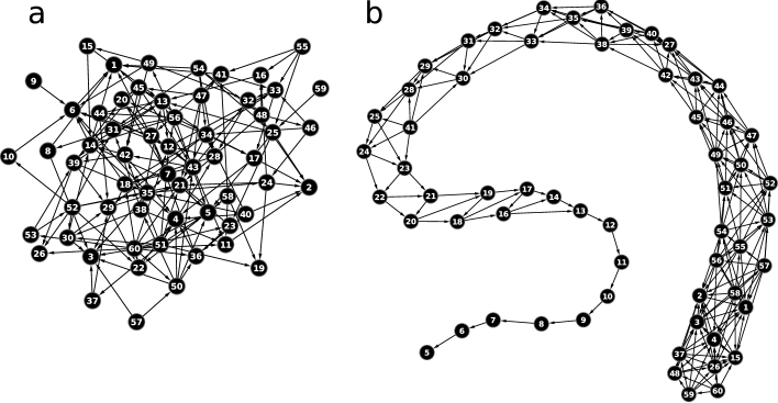
Figure 2: Illustration of a Random-DAG with $N=60$ and $\langle k\rangle=3$ (a). Illustration of a Snake-DAG with $N=60$ and $K=6$ (b). In both graphs arrows go from nodes with larger numbers to nodes with smaller number.

Table 1: Joint entropy values for a Random-DAG of $|V|=600$ and $|E|=6000$ and a set of $500$ randomized graphs after $2^{18}$ iterations of each of the four randomization methods (alphabetically denoted). Symbol (^∗) denotes significant differences.

method	${\cal D}$	$H^{u}({\cal G}_{u}^{t})$	$H^{i,o}({\cal G}^{t})$	$H^{i,i}({\cal G}^{t})$	$H^{o,o}({\cal G}^{t})$
${\cal G}$ orig.	-	8.279	9.214	9.163	9.250
${\mathbf{a}}$	0.98	8.283 $\pm$ 0.003 (Z=-1.67)	9.21 $\pm$ 0.02 (Z=0.25)	9.20 $\pm$ 0.04 (Z=-0.95)	9.21 $\pm$ 0.04 (Z=1.01)
${\mathbf{b}}$	0.98	8.283 $\pm$ 0.003 (Z=-1.46)	9.21 $\pm$ 0.03 (Z=0.21)	9.20 $\pm$ 0.04 (Z=-0.90)	9.21 $\pm$ 0.04 (Z=1.02)
${\mathbf{c}}$	0.96	8.282 $\pm$ 0.003 (Z=-1.03)	9.209 $\pm$ 0.003 (Z=1.92)	9.157 $\pm$ 0.004 (Z=1.76)	9.249 $\pm$ 0.004 (Z=0.03)
${\mathbf{d}}$	0.96	8.281 $\pm$ 0.003 (Z=-0.62)	9.206 $\pm$ 0.002 (Z=2.96)	9.152 $\pm$ 0.004 (Z=3.03)	9.247 $\pm$ 0.004 (Z=0.68)

Table 2: Joint entropy values for a snake-DAG ($|V|=600$ and $K=6$) and a set of $500$ randomized graphs after $2^{18}$ iterations of each of the four randomization methods (alphabetically denoted). Symbol (^∗) denotes significant differences.

method	${\cal D}$	$H^{u}({\cal G}_{u}^{t})$	$H^{i,o}({\cal G}^{t})$	$H^{i,i}({\cal G}^{t})$	$H^{o,o}({\cal G}^{t})$
${\cal G}$ orig.	-	2.998	4.331	4.131	4.161
${\mathbf{a}}$	0.99	5.281 $\pm$ 0.003 (Z=-691.88∗)	6.98 $\pm$ 0.02 (Z=-152.2∗)	6.97 $\pm$ 0.03 (Z=-91.53∗)	6.97 $\pm$ 0.03 (Z=-86.86∗)
${\mathbf{b}}$	0.99	5.281 $\pm$ 0.003 (Z=-671.59∗)	6.98 $\pm$ 0.02 (Z=-174.3∗)	6.97 $\pm$ 0.03 (Z=-91.83∗)	6.97 $\pm$ 0.03 (Z=-92.05∗)
${\mathbf{c}}$	0.95	4.96 $\pm$ 0.03 (Z=-58.88∗)	5.37 $\pm$ 0.02 (Z=-52.96∗)	5.50 $\pm$ 0.02 (Z=-63.42∗)	5.12 $\pm$ 0.02 (Z=-42.22∗)
${\mathbf{d}}$	0.93	4.71 $\pm$ 0.03 (Z=-51.63∗)	5.15 $\pm$ 0.02 (Z=-43.89∗)	5.22 $\pm$ 0.03 (Z=-41.95∗)	5.05 $\pm$ 0.02 (Z=-40.23∗)

IV.2 Extreme Graphs

Prior to evaluate the randomness of real DAGs, we construct two extreme topologies in order to evaluate the behavior of the algorithms using the measures defined above. The first model, random-DAG, permit us to test the randomization methods in a highly disordered degree-degree scenario. In terms of degree-degree joint entropy, minimal changes are expected along the randomization processes. The second model, snake-DAG, permit us the same test but in a highly ordered scenario where large increments of joint entropy values should be observed.

IV.2.1 random-DAG model

The first one is a completely degree-degree disordered DAG, up to finite size effects. Let $V$ be a set of $N$ nodes, by which the probability for two of them to be connected is constant and equal to $p$. This is the definition of the Erdös Rényi (ER) graph. Once we have an ER graph, we randomly label the nodes of $V$ sequentially, from $1$ to $N$. Finally, we define the direction of the arrows by looking at the labeling of the nodes and observing condition (1). We will refer to this model as random-DAG.

We created a random-DAG of $|V|=600$ and $|E|=6000$ and, for each method, an ensemble of $500$ randomized graphs product of $2^{18}$ iterations. See fig. (2a) for an example of this graph. As shown in Table 1, none of the degree-degree relations of the random-DAG where neither significantly low nor significantly high with respect to any of its randomized ensembles. This result indicates that the four randomization methods proposed here do not produce significant undesirable biases in the degree-degree almost null relations of a originally random-DAG.

IV.2.2 snake-DAG model

Opposed to the random-DAG model, we construct a highly degree-degree ordered acyclic graph, which we will call snake-DAG see fig. (2). In this graph, nodes of the same degree tend to be connected among them, giving rise to a high degree-degree relation and thus very low joint entropy values. In the following lines we outline the construction of this network.

Let us consider $K\equiv k_{o}^{max}$ as the highest outdegree to appear in the resulting graph. Let $V$ be the set of nodes such that there exists an integer $n$ by which $n\cdot K=|V|$. We then perform a partition of $V$ in $K$ different subsets

$${\cal P}(V)=\{V_{1},...,V_{K}\}.$$ (18)

In this partition, for any $V_{i}\in{\cal P}(V)$, $|V_{i}|=n$. We sequentially number the nodes of the set $V$ is the following way: For the subset of nodes $V_{1}$, the label will run from $1$ to $n$, thus obtaining:

$$V_{1}=\{v_{1},...,v_{n}\}$$

For the subset of nodes $V_{2}$, the label will run from $n+1$ to $2n$:

$$V_{2}=\{v_{n+1},...,v_{2n}\}.$$

We follow the numbering by using the criteria that the nodes of subset $V_{i}$ will be labeled from $(i-1)n+1$ to $i\cdot n$, until all the nodes of $V$ are numbered. We then identify the label of the partition with the out-degree of the nodes belonging to it, namely:

$$(v_{i}\in V_{m})\Rightarrow(k_{o}(v_{i})=m).$$ (19)

Now we proceed to define the connections: For any $v_{i}\in V_{m}$, we will have the following links $\langle v_{i},v_{i-1}\rangle,...,\langle v_{i},v_{i-m}\rangle$. This process excludes node $v_{1}$ which will only receive a link from $v_{2}$. We observe that, in general, both $v_{1}$ and $v_{2}$ belong to $V_{1}$. Finally, to break the extreme symmetry of the obtained net, we introduce a minimal source of noise by renumbering a small fraction $\sim 0.05$ of the nodes with a further arrow orientation consistently with the new numbering, as depicted in eq. (1).

Analogous to the experiment performed with a random-DAG, we create a snake-DAG of $|V|=600$ and $|E|=2099$ ($K=6$) and, for each method, an ensemble of $500$ randomized graphs product of $2^{18}$ iterations. See fig. (2b) for an example of this graph. As shown in Table 2, all the degree-degree relations of the snake-DAG were significantly high with respect to any of the randomized ensembles. This result indicates that the four randomization methods proposed here are able to successfully deteriorate the high degree-degree relations present at the snake-DAG.

IV.3 Real biological and social DAGs

Results of previous section have checked the behavior of the four methods in two toy models with high and low degree-degree relations respectively. In this section we proceed to evaluate three DAGs representing real systems: the C. elegans cell lineage network, the Milgram’s citation network and a PhD student-advisor network.

IV.3.1 C. elegans cell lineage network

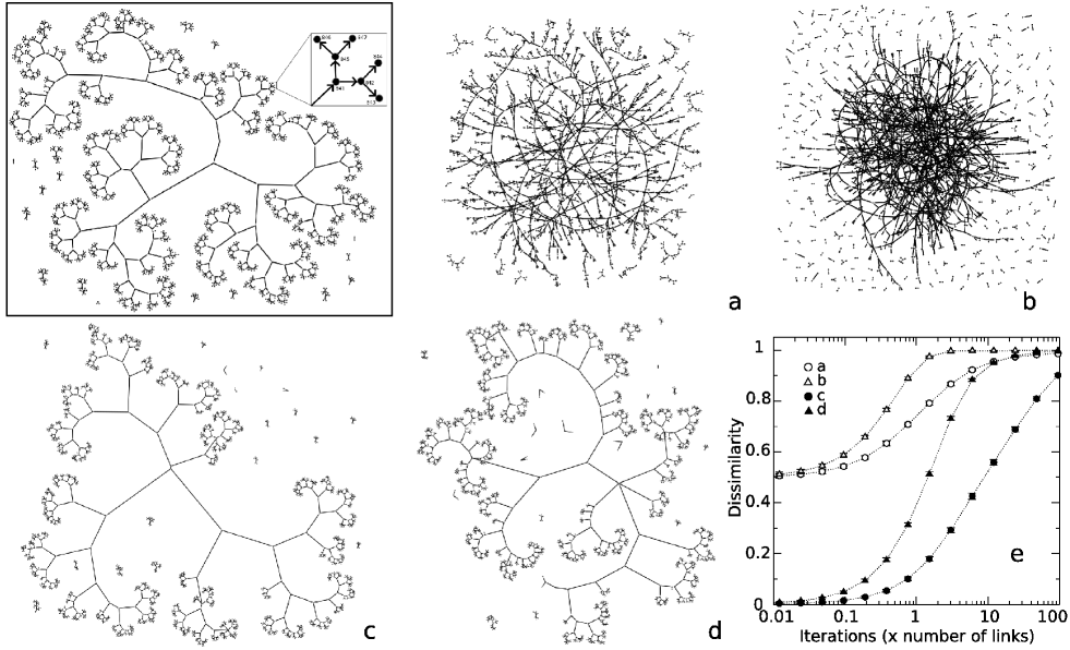
Figure 3: DAG representation of the cell lineage of Caebnorhabditis elegans (inbox). A prototypic randomized network after $2^{18}$ iterations is present for each method: randomization preserving undirected degree sequence and component size distribution (a), randomization only preserving the undirected degree sequence (b), randomization preserving directed degree sequence and component size distribution (c) and randomization preserving only directed degree sequence (d). Panel (e) represents the dissimilarity preserving the original network along the process of randomization for every randomization type. The mean and the standard deviation of $500$ graph randomizations are shown for each point.

Table 3: Joint entropy values for the original C. elegans network and a set of $500$ randomized networks after $2^{18}$ iterations of each of the four randomization methods (alphabetically denoted). Symbol (^∗) denotes significant differences and (^a) denotes that Z-score is not computable due to $\sigma=0$

method	${\cal D}$	$H^{u}({\cal G}_{u}^{t})$	$H^{i,o}({\cal G}^{t})$	$H^{i,i}({\cal G}^{t})$	$H^{o,o}({\cal G}^{t})$
${\cal G}$ orig.	-	1.832	0.991	0.116	1.732
${\mathbf{a}}$	0.99	1.833 $\pm$ 0.001 (Z=-0.58)	3.71 $\pm$ 0.01 (Z=-205.9∗)	3.67 $\pm$ 0.02 (Z=-167.4∗)	3.66 $\pm$ 0.02 (Z=-92.88∗ )
${\mathbf{b}}$	1.00	1.961 $\pm$ 0.001 (Z=-117.3∗)	3.71 $\pm$ 0.01 (Z=-224.5∗)	3.69 $\pm$ 0.02 (Z=-175.0∗)	3.68 $\pm$ 0.02 (Z=-92.55∗)
${\mathbf{c}}$	0.90	1.831 $\pm$ 0.002 (Z=0.41)	0.990 $\pm$ 0.001 (Z=1.33)	0.116 $\pm$ 0.0a	1.736 $\pm$ 0.002 (Z=-2.67)
${\mathbf{d}}$	0.99	1.832 $\pm$ 0.002 (Z=0.80)	0.989 $\pm$ 0.001 (Z=-1.6)	0.116 $\pm$ 0.0a	1.734 $\pm$ 0.002 (Z=-1.67)

The first system chosen is a cell lineage network. Briefly, it captures the genealogic pedigree of cells related through mitotic division during its development in a tree-like structure. The cell lineage network of C. elegans was retrieved from the WormBase  C. elegans repository. In this network the initial egg division (the giant component) and alternative variants of neural post-embrionic cell lines are included in a 18-component graph representation. All the randomization methods were applied up to $2^{18}$ iterations. The dissimilarity values reached were over $0.90$ in all cases, indicating a successful alteration of most of the links under the different topological invariants.

Figure (3) shows the original and a representative DAG for each randomization method. Note the deep fragmentation produced by method ${\mathbf{b}}$, where only the undirected degree sequence is preserved ($205$ components in fig. (3b) against 18-component in the original graph). Interestingly, figure (3 d) shows that the tree-like structure and the number of graph components are conserved by just only preserving the directed degree sequence invariant. The reason is that the regular pattern of $k_{i}=1$ for all non-maximal nodes in its directed degree sequence is graphical only in a tree structure. In this particular situation the number of DAG components coincides with the number of maximal nodes. However, the size of components is not strictly conserved and this condition is only possible by applying the local-swap as observed in figures 3a and 3c.

Looking at figure (3e), all randomizations provide completely re-allocation of nodes. It is worth to note that methods not preserving the directed degree sequence start with a dissimilarity values of around $0.5$. The reason is that a complete random arrow orientation occurs for every iteration. This contrasts with methods ${\mathbf{c}}$ and ${\mathbf{d}}$ where rewiring operated over the directed graph. Table (3) shows that almost all the ensembles generated through the proposed algorithms display relevant deviations in the values of joint entropies. They are higher than the observed in the real DAG when the undirected degree sequence is preserved (methods $\mathbf{{a},{b}}$). Otherwise, when the directed degree sequence is conserved, no deviations are found (methods $\mathbf{{c},{d}}$) due to the very restrictive (even zero) standard deviations.

IV.3.2 Milgram’s citation network

The second system is a sample of the process of article citation. The chosen system used to illustrate this process is the resulting network containing the papers that cite ”S Milgram’s 1967 Psychology Today” paper or use Small World in the title. This network was retrieved from to Pajek’s network dataset . All the randomization methods were applied up to $2^{18}$ iterations (see figure 4). The dissimilarity values reached were over $0.86$ for methods ${\mathbf{a}}$ and ${\mathbf{b}}$ and over $0.76$ for methods ${\mathbf{c}}$ and ${\mathbf{d}}$. This indicates that keeping the directed degree sequence as a topological invariant reduces the heterogeneity of feasible graphs and thus the dissimilarity reached.

Table (4) shows significantly low joint-entropy values, indicating that this DAG displays a statistically relevant undirected degree-degree relation respect to all their randomized ensembles. It can also be appreciated relevant indegree-outdegree and outdegree-outdegree relations with respect to all their randomized ensembles. In the case of indegree-indegree entropies, it shows a high degree-degree relation respect to the randomized ensembles produced by methods ${\mathbf{a}}$ and ${\mathbf{b}}$, while there were no differences respect to the randomized ensembles produced by methods ${\mathbf{c}}$ and ${\mathbf{d}}$. This result indicates that indegree-indegree relations in the Milgram’s citation network are high respect to the random DAGs that preserve only the undirected degree sequence and not differentiable from the ones obtained by preserving the directed degree sequence.

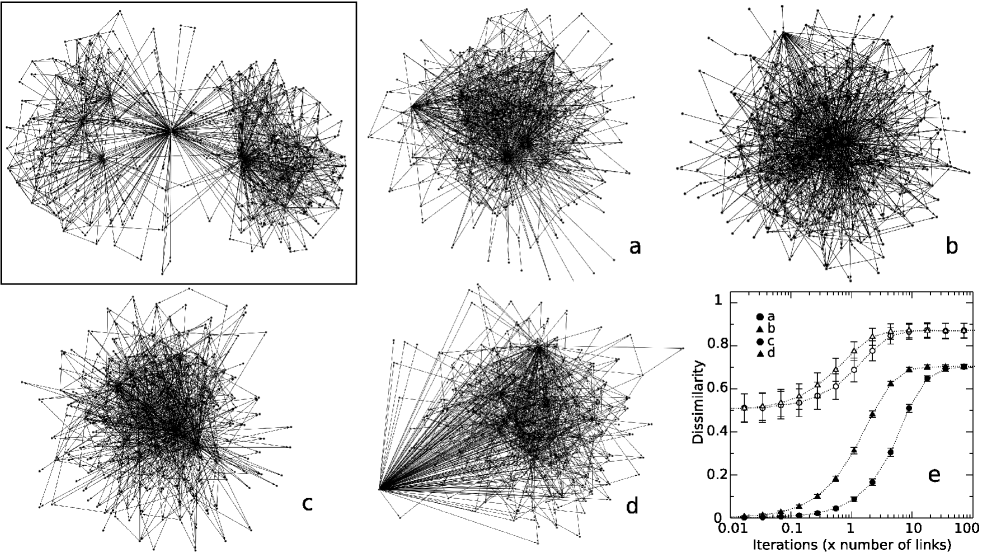
Figure 4: DAG representation of the Milgram’s citation network (inbox). A prototypic randomized network after $2^{18}$ iterations is present for each method: randomization preserving undirected degree sequence and component size distribution (a), randomization only preserving the undirected degree sequence (b), randomization preserving directed degree sequence and component size distribution (c) and randomization preserving only directed degree sequence (d). Panel (e) represents the dissimilarity respecting the original network along the process of randomization for every randomization type. The mean and the standard deviation of $500$ graph randomizations are shown for each point.

Table 4: Joint entropy values for the original Milgram’s citation network and a set of $500$ randomized networks after $2^{18}$ iterations of each of the four randomization methods (alphabetically denoted). Symbol (^∗) denotes significant differences.

method	${\cal D}$	$H^{u}({\cal G}_{u}^{t})$	$H^{i,o}({\cal G}^{t})$	$H^{i,i}({\cal G}^{t})$	$H^{o,o}({\cal G}^{t})$
${\cal G}$ orig.	-	9.03	7.38	7.16	7.53
${\mathbf{a}}$	0.87	9.24$\pm$ 0.02 (Z=-10.5∗)	8.2 $\pm$ 0.1 (Z=-8.6∗)	8.2 $\pm$ 0.1 (Z=-7.8∗)	8.20 $\pm$ 0.1 (Z=-4.8∗)
${\mathbf{b}}$	0.87	9.24 $\pm$ 0.02 (Z=-10.5∗)	8.2 $\pm$ 0.1 (Z=-8.6∗)	8.2 $\pm$ 0.1 (Z=-7.6∗)	8.22 $\pm$ 0.1 (Z=-5.1∗)
${\mathbf{c}}$	0.70	9.18 $\pm$ 0.02 (Z=-7.35∗)	7.45 $\pm$ 0.01 (Z=-7.38∗)	7.17 $\pm$ 0.01 (Z=-1.42)	7.63 $\pm$ 0.01 (Z=-8.59∗)
${\mathbf{d}}$	0.70	9.18 $\pm$ 0.02 (Z=-7.93∗)	7.45 $\pm$ 0.01 (Z=-7.34∗)	7.17 $\pm$ 0.01 (Z=-1.40)	7.63 $\pm$ 0.01 (Z=-8.63∗)

This example illustrates how a randomization process destroys local associations and the heterogeneous partition observed in the original DAG (figure 4 inbox). In this case, due to the high connectivity of the original DAG, -it is worth to note that such a graph contains several nodes whose connectivity is ${\cal O}(|V|)$- fragmentation is unlike to happen due to a high average connectivity. Furthermore, as a side effect, an upper boundary below maximal value of dissimilarity is imposed depending on the randomization method used. This is due to a considerable fraction of failed rewiring attempts. An example of that is provided by a clique conformation where no rewiring is possible. In this case no effective of rewiring can be done since all possible link combinations satisfying the directed acyclic condition are actually in the network.

IV.3.3 PhD student-advisor network

The last system evaluated in this paper contains the ties between PhD students and their advisors in theoretical computer science. Each arc points from an advisor to a student. Data was retrieved from to Pajek’s network dataset . This network illustrates just the intermediate situation between the two previous examples. It is a DAG able to be fragmented (when DAG components conservation is not imposed) but with just right connectivity: too low to avoid fragmentation but not too high to impose an upper bounding in dissimilarity, being, jointly to the random-DAG studied above, the DAG structure closer to the assumptions of the configuration model. Interestingly, contrasting with the C. elegans case, network fragmentation also occurs when preserving directed degree sequence but not when the component distribution conservation is preserved. All the randomization methods were applied up to $2^{18}$ iterations. The dissimilarity values reached where over $0.97$ in all cases, indicating a successful alteration of most of the links under the different topological invariants.

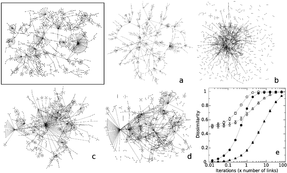
Figure 5: DAG representation of PhD advisors (inbox). A prototypic randomized network after $2^{18}$ iterations is present for each method: randomization preserving undirected degree sequence and component size distribution (a), randomization only preserving the undirected degree sequence (b), randomization preserving directed degree sequence and component size distribution (c) and randomization preserving only directed degree sequence (d). Panel e represents the dissimilarity respecting the original network along the process of randomization for every randomization type. The mean and the standard deviation of $500$ graph randomizations are shown for each point.

Table 5: Joint entropy values for the PhD student-advisor network a set of $500$ randomized networks after $2^{18}$ iterations of each of the four randomization methods (alphabetically denoted). Symbol (^∗) denotes significant differences.

method	${\cal D}$	$H^{u}({\cal G}_{u}^{t})$	$H^{i,o}({\cal G}^{t})$	$H^{i,i}({\cal G}^{t})$	$H^{o,o}({\cal G}^{t})$
${\cal G}$ orig.	-	6.42	4.075	1.348	6.34
${\mathbf{a}}$	0.99	6.47 $\pm$ 0.01 (Z=-4.50)	5.67 $\pm$ 0.06 (Z=-26.06∗)	5.58 $\pm$ 0.1 (Z=-36.07∗)	5.56 $\pm$ 0.1 (Z=6.70∗)
${\mathbf{b}}$	0.99	6.75 $\pm$ 0.01 (Z=-29.62∗)	5.69 $\pm$ 0.06 (Z=-28.68∗)	5.63 $\pm$ 0.1 (Z=-43.18∗)	5.62 $\pm$ 0.1 (Z=7.46∗)
${\mathbf{c}}$	0.97	6.47 $\pm$ 0.01 (Z=-5.34)	4.076 $\pm$ 0.005 (Z=-0.32)	1.31 $\pm$ 0.01 (Z=3.33∗)	6.39 $\pm$ 0.01 (Z=-4.53∗)
${\mathbf{d}}$	0.98	6.59 $\pm$ 0.01 (Z=-13.55∗)	4.072 $\pm$ 0.005 (Z=0.63)	1.366 $\pm$ 0.002 (Z=-8.27∗)	6.39 $\pm$ 0.01 (Z=-5.13∗)

Table 5 displays statistically significant low joint-entropy values, indicating that this DAG has relevant undirected degree-degree relations with respect to all their randomized ensembles. It also displays a statistically relevant indegree-indegree and outdegree-outdegree relations with respect to all their randomized ensembles. In the case of indegree-outdegree, it shows significant relations with respect to the randomized ensembles produced by methods ${\mathbf{a}}$ and ${\mathbf{b}}$, while there were no differences respect to the randomized ensembles produced by methods ${\mathbf{c}}$ and ${\mathbf{d}}$. This result indicates that indegree-outdegree relations in the PhD student-advisor network are high with respect to the random DAGs that preserve only the undirected degree sequence and are not differentiable from the ones obtained by random DAGs that also preserve the directed degree sequence.

V Discussion

In this paper we present a set of four algorithms based on an iterative process of rewiring for the construction of DAG random models. The difference between algorithms stems from two topological invariants under consideration, namely, the conservation of the directed degree sequence and/or the conservation of the connected component distribution. In contrast to other methods of random model construction, this approach works within the space of graphical solutions providing a feasible computational approximation for the exploration of such a graphical space considering a defined number of topological invariants in the null-model ensemble generation.

Our methodology was evaluated through the analyses of both extreme and real graphs comparing them with their associated randomized ensembles using two measures: dissimilarity and joint entropy. While the former indicates whether connections are actually changed after randomization, the latter quantifies the disorder or uncertainty in the degree-degree relations, thereby being an indicator of randomness. In this context, it is worth to mention that other measures such assortative mixing Newman (2002); Foster et al. (2009) or mutual information Sole and Valverde (2004) have been suggested for the evaluation of degree-degree relations. In essence, these measures compare the actual degree correlations relation in the graph with the expected one obtained from the remaining degree information. A problem arises when a proper definition of remaining degree attending directedness needs of the information of the directed degree sequence because of the latter is a topological feature not preserved in all of our methods (methods ${\mathbf{a}}$ and ${\mathbf{b}}$). Therefore, measures based on remaining degree information, although extensively used as estimators of degree-degree relations in the network literature Newman (2002); Foster et al. (2009); Sole and Valverde (2004) cannot be applied in this work for a comparative evaluation of our methodology.

To overcome these limitations, joint entropy was used as a raw measure of uncertainty once defined to be applied to directed graphs leading to four alternative descriptors according to in and out-degree information. Furthermore, the significance of the variation of degree-degree relations between the random ensembles and the original graph was evaluated using a Z-score estimator. The analysis of network models verified that our methods do not produce a bias when applied to the random-DAG model whilst they produced a significative increase of disorder of the degree-degree relations on the snake-DAG model when randomized -see table 2. Going to real systems, our analyses revealed that all the methods produced an $H^{u}$ greater than its respective original value, suggesting that randomizations disorder the underlying graph and they do not only affect the pattern of arrows. However, values of undirected joint entropies are different among methods, suggesting that conservation of the DAG condition and the remaining topological invariants have a variable impact on the underlying network. When we look at the directed joint entropies a general increase of the values was observed for all of methods, although some exceptions are observed. This is the case of PhD student-advisor network where the original network exibits a diversity of degree-degree relations higher than the randomized ensemble.

Additionaly, our results show that preserving the component size structure is an important aspect to take into account since it has drammatic effects when the network is markedly sparse. This is the case of C. elegans and PhD student-advisor DAGs by which randomizations not preserving the component size produced a graph fragmentation. On the contrary, high average degree guarantees the preservation of the giant component and randomization methods. In such circumstances, methods ${\mathbf{a}}$ and ${\mathbf{b}}$ give comparable values of joint entropies. Analogously, this is also sobserved for method ${\mathbf{c}}$ and ${\mathbf{d}}$ (see joint entropy for network models and also for the Milgram’s citation network). This feature indicates that the conservation of component structure premise is not relevant and produce indistinguisable topologies when graph fragmentation is unlike to happen.

Another important observation is related to the small values displayed by standard deviations in joint entropies. For methods ${\mathbf{c}}$ and ${\mathbf{d}}$ are one order of magnitud lower than the ones obtained for methods ${\mathbf{a}}$ and ${\mathbf{b}}$ . It suggests that just directed degree sequence conservation is enough to severely reduce the space of graphical configurations. Consistenly, it was observed that, in general, methods ${\mathbf{c}}$ and ${\mathbf{d}}$ provided lower Z-values than ${\mathbf{a}}$ and ${\mathbf{b}}$. However, the small divergence of the obtained values is not explained by a non-effective rewiring since high values of dissimilarity were reached. An interesting exception was found in the Milgram’s citation network where dissimilarity values after processes of randomization were markedly lower than the observed in the other real networks, as well as in the toy models. An explanation can be found in the presence of superhubs, nodes whose connectivity is $\sim{\cal O}(|V|)$. This introduces a strong constraint in the rewiring, difficult -even impossible- to overcome. Nevertheless figure (4) illustrates that the original network seems to be partitioned in two regions. Using the same layout for randomized graphs, we observed that such a partition was lost, suggesting that rewiring process was accounted. Contrasting to this behaviour, C. elegans randomized ensembles were completely suffled -as indicated by the high values of dissimilarity- but degree-degree relations were not always significatively altered. This is specially evident when directed degree sequence is conserved. An explanation can be obtained by the fact that this DAG is practically a dichotomic tree. This network is sparse enough to be fragmented as it happened in method ${\mathbf{b}}$. Nevertheless, preserving its extremal directed degree sequence was enough to conserve the number of components (not their size though). This is in aggreement to the constraint in the number of DAG components described in eq. (7). In fact, this is a result of the limited space of possibilities permited by the extremal directed degree sequence and therefore very little variation is found in the joint entropies (notice the case of zero $H^{i,i}$ for method ${\mathbf{c}}$). Interestingly, when directed degree sequence and component structure are not preserved, tree configuration is unlikely to happen by chance. However, tree structure is practically the only solution when directed degree sequence is preserved even not conserving the component size distribution.

The choice of topological constraints (i.e. the particular method ) for a desired randomization process depends upon the question the researcher wants to explore, rather than upon a technical issue. Preserving the directed degree sequence captures the need to fix the number of inputs and outputs for every element. Randomizations attending to this constraint (for example, in a technological system) may be interpreted as a rewiring of an electronic circuit by a random assembling of integrated devices (e. g. chips) but respecting the inputs and outputs of the components. This contrasts with the softer undirected degree sequence invariant produced by preserving just the number of connections in every node. In this case, the relevance relies on the number of relations instead of mattering the arrows orientation -i.e., the undirected degree sequence. Furthermore, the conservation of the connected components is essential in a graph describing a process, since fragmentation can be intepreted as a break of the flow of causality.

Finally, we stress that an important feature of any randomization process is that topological invariants restrict the space of graphical solutions. Our methodology provides valuable information about the randomness of a particular structure within the context of its graphical space of solutions. It is arguable to think that the higher the number of constraints the smaller the space of solutions. In any case, its complete exploration is not feasible beyond a graph containing more than a handful of nodes. In this context, our methodology provides a sampling of such space in order to estimate the randomness of a DAG given some topological contraints

VI Acknowledgements

This work was supported by the EU $6^{th}$ framework project ComplexDis (NEST-043241, CRC and JG), the UTE project CIMA (JG), James McDonnell Foundation (BCM and RVS) and Santa Fe Institute (RVS) We thank Complex System Lab members for fruitful conversations.

References

- Watts and Strogatz (1998) D. J. Watts and S. H. Strogatz, Nature 393, 440 (1998).
- Newman et al. (2001) M. E. J. Newman, S. H. Strogatz, and D. J. Watts, Phys. Rev. E 64, 026118 (2001).
- Dorogovtsev and Mendes (2003) S. N. Dorogovtsev and J. F. F. Mendes, Evolution of networks. From Biological nets to the Internet and WWW (Oxford University Press. Oxford UK, 2003).
- Sole et al. (2003) R. V. Sole, R. Ferrer-Cancho, J. M. Montoya, and S. Valverde, Complexity 8, 20 (2003).
- Boccaletti et al. (2006) S. Boccaletti, V. Latora, Y. Moreno, M. Chavez, and D.-U. Hwang, Physics Reports 424, 175 (2006).
- Hummon and Doreian (1989) N. Hummon and P. Doreian, Social Networks 11, 39 (1989).
- E. et al. (1964) G. E., I. H. Sher, and R. J. Torpie., Tech. Rep., Published by The Institute for Scientific Information. Report of research for Air Force Office of Scientific Research under contract F49(638)-1256. (1964).
- Valverde et al. (2007) S. Valverde, R. V. Sole, M. A. Bedau, and N. Packard, Phys Rev E Stat Nonlin Soft Matter Phys 76, 056118 (2007).
- Csardi et al. (2007) G. Csardi, K. J. Strandburg, L. Zalanyi, J. Tobochnik, and P. Erdi, Physica A 374, 783 (2007).
- Fowler and Jeon (2008) J. H. Fowler and S. Jeon, Social Networks 30, 16 (2008).
- Chandler (2005) S. J. Chandler, The University of Houston Working Paper Series. Public Law and Legal Theory Series pp. 2005–W–01 (2005).
- Clay (1971) R. Clay, Nonlinear networks and systems (John Wiley & Sons Inc, New York, 1971).
- Haykin (1999) S. Haykin, Neural Networks : a Comprehensive Foundation (Prentice-Hall. London, 1999).
- Frank and Frisch (1971) H. Frank and I. T. Frisch, Communication, transmission and transportation networks (Addison-Wesley (Reading Mass), 1971).
- Fulton et al. (2001) W. Fulton, A. Katok, F. Kirwan, P. Sarnak, B. Simon, and B. Totaro, eds., Random Graphs (Cambridge University Press, 2001).
- Molloy and Reed (1995) M. Molloy and B. Reed, Random Structures and Algorithms 6, 161 (1995).
- Karrer and Newman (2009) B. Karrer and M. E. J. Newman, Phys Rev Lett 102, 128701 (2009).
- Aiello et al. (2001) W. Aiello, F. Chung, and L. Lu, in Proceedings of the Thirty-Second Annual ACM Symposium on Theory of Computing (2001), pp. 171–180.
- Maslov and Sneppen (2002) S. Maslov and K. Sneppen, Science 296, 910 (2002).
- Han (2009) Randomization Techniques for Graphs (2009).
- Suppes (1960) P. Suppes, Axiomatic Set Theory (Dover. New York, 1960).
- Kelley (1955) J. Kelley, General Topology, Graduate Texts in Mathematics, 27, 1975 (Van Nostrand, 1955).
- Rodriguez-Caso et al. (2009) C. Rodriguez-Caso, B. Corominas-Murtra, and R. V. Sole, Mol Biosyst 5, 1617 (2009).
- Shannon (1948) C. E. Shannon, Bell System Technical Journal 27, 379 (1948).
- Newman (2002) M. E. J. Newman, Phys. Rev. Lett. 89, 208701 (2002).
- Foster et al. (2009) J. G. Foster, D. V. Foster, P. Grassberger, and M. Paczuski, arXiv (2009).
- Sole and Valverde (2004) R. V. Sole and S. Valverde, in Complex Networks (Lecture Notes in Physics, Springer-Verlag, 2004), pp. 189–210.