Dynamical $p$-branes with a cosmological constant

Abstract

We present a class of dynamical solutions in a $D$-dimensional gravitational theory coupled to a dilaton, a form field strength, and a cosmological constant. We find that for any $D$ due to the presence of a cosmological constant, the metric of solutions depends on a quadratic function of the brane world volume coordinates, and the transverse space cannot be Ricci flat except for the case of 1-branes. We then discuss the dynamics of 1-branes in a $D$-dimensional spacetime. For a positive cosmological constant, 1-brane solutions with $D>4$ approach the Milne universe in the far-brane region. On the other hand, for a negative cosmological constant, each 1-brane approaches the others as the time evolves from a positive value, but no brane collision occurs for $D>4$, since the spacetime close to the 1-branes eventually splits into the separate domains. In contrast, the $D=3$ case provides an example of colliding 1-branes. Finally, we discuss the dynamics of 0-branes and show that for $D>2$, they behave like the Milne universe after the infinite cosmic time has passed.

I Introduction

Supergravity is an important framework to study spacetime-dependent solutions and their application to cosmology, because it is a low-energy effective theory of superstrings. Spacetime-dependent brane solutions in supergravity theories have played an important role in the development of higher-dimensional gravity theory Lu:1996jk ; Lu:1996er ; Chen:2002yq ; Ohta:2003uw ; Gibbons:2005rt ; Kodama:2005fz ; Kodama:2005cz ; Binetruy:2007tu ; Ishino:2005ru ; Maeda:2009tq ; Maeda:2009zi ; Maeda:2009ds ; Gibbons:2009dr ; Maeda:2010yk ; Maeda:2010ja . Their central importance in supergravity theory can be anticipated in their applications to cosmology and dynamical black holes.

The time-dependent generalizations of single static $p$-brane solutions were discussed in Lu:1996jk ; Lu:1996er ; Chen:2002yq ; Ohta:2003uw . Those with dependence on both time and space have been first discussed in the case of a ten-dimensional type IIB supergravity model Gibbons:2005rt . The extension of static solutions Ohta to the spacetime-dependent case for $p$-brane and intersecting branes in the ten- or eleven-dimensional supergravity are now well understood Binetruy:2007tu ; Ishino:2005ru ; Maeda:2009tq ; Maeda:2009zi . In particular, the explicit form of the warp factor in the metric has been obtained. The solutions are specified by the choice of the scalar and gauge fields and the values of the exponent in the warp factor of the metric. The solutions give the Friedmann-Lemaître-Robertson-Walker (FLRW) universe when we regard the homogeneous and isotropic part of the brane world volume as our four-dimensional spacetime, whereas they provide black hole solutions in a FLRW universe when we regard the bulk transverse space as our three-dimensional space  Maeda:2009zi ; Maeda:2009ds . It was found that the warp factor in the metric is a linear function of the time except for the trivial or vanishing dilaton, and then even for the fastest expanding case, the power is too small to give a realistic expansion law as in the matter dominated era or in the radiation dominated era Binetruy:2007tu ; Maeda:2009zi . In order to find a realistic cosmic expansion, we have to include additional matter fields. Note that no cosmological constant is considered in these solutions.

In another line of development, the dynamical solutions in six-dimensional Nishino-Salam-Sezgin (NSS) supergravity theory Nishino:1984gk ; Salam:1984cj ; Nishino:1986dc ; Gibbons:2003di ; Aghababaie:2003ar with a positive cosmological constant have been investigated in Maeda:1984gq ; Maeda:1985es ; tbdh1 ; tbdh2 ; Minamitsuji:2010fp , including applications to brane world models. An application of a static solution in the six-dimensional Romans supergravity romans1 ; romans2 (with a negative cosmological constant) to brane world model was also discussed in Aghababaie:2003ar . These solutions are considerably different from the above class of solutions because of the presence of the cosmological constant. Some arguments on the origin of the cosmological constant in the context of string theory are given in AGMV ; POL . These dynamical solutions cannot be in general derived from the ordinary ansatz of fields used in a $p$-brane system. One particular construction of dynamical solutions was discussed recently in the NSS model and then applied to brane world models in Minamitsuji:2010fp . In the present paper, dynamical 1-brane solutions in the NSS model and in a class of the six-dimensional Romans supergravity will be derived and used to understand the brane collisions. Brane collisions in the special case of $p$-branes have been originally discussed in Gibbons:2005rt .

The main purpose of the present paper is to unify these two lines of development, by showing that the methods that have already been used in analyzing the dynamical $p$-brane system without the cosmological constant lead naturally to the extension of $p$-branes in theories with the cosmological constant. We show that quadratic functions of the time, more precisely of the world volume coordinates, appear in the solutions as the warp factor due to the contribution of a cosmological constant. These are similar to the dynamical solutions without a cosmological constant with a trivial or vanishing dilaton found in Binetruy:2007tu . We apply the resulting dynamical solutions to brane collision and cosmology. We also find that the dynamical 0-brane solution describes the Milne universe.

This paper is organized as follows. In Sec. II, we argue that there exists a procedure allowing one to construct dynamical $p$-brane solutions with a cosmological constant in a $D$-dimensional theory which generalizes the approach in Minamitsuji:2010fp , and discuss their applications. First in Sec. II.1, we introduce our theory and derive the basic equations, and reduce them to a set of simple equations which should be satisfied for dynamical $p$-brane solutions. They are given without specifying the brane world volume and other part of the spacetime. We find that the basic difference of the solutions is that they involve Einstein space for a nonvanishing cosmological constant, except for $p=1$ and $p=0$. Secondly, in Sec. II.2, we discuss the behavior of multiple 1-branes in our broad class of solutions in the $D$-dimensional theory and show that the solutions have interesting behaviors. For a positive cosmological constant and $D>4$, 1-brane solutions approach the Milne universe in the far region. For a negative cosmological constant, the spacetime starts with the structure of combined 1-branes, but a part of it eventually splits into separate regions as the time increases from zero for $D>4$, which is similar to the result in Gibbons:2005rt . Thus, 1-branes never collide. In contrast, the case of $D=3$ provides an example of colliding branes. Finally, in Sec. II.3, we discuss the dynamical 0-brane solutions in the context of cosmology and show that they give the Milne universe in $D>2$ dimensions. Section III is devoted to our conclusions.

II Dynamical $p$-brane solutions with a cosmological constant

In this section, we consider dynamical $p$-brane solutions in theories with the cosmological constant in $D$ dimensions. First, we write down the equations of motion under a particular ansatz for the metric, which is a generalization of the known static $p$-brane solutions. Then, we solve the equations of motion and present the solutions explicitly for the cases of $p=1$ and 0.

II.1 Basic equations and “general” solutions

We consider a gravitational theory with the metric $g_{MN}$, the dilaton $\phi$, the cosmological constant $\Lambda$, and the antisymmetric tensor field of rank $(p+2)$, $F_{(p+2)}$. The action which we consider is given by

$$S=\frac{1}{2\kappa^{2}}\int\left[\left(R-2{\rm e}^{\alpha\phi}\Lambda\right)\ast{\bf 1}_{D}-\frac{1}{2}d\phi\wedge\ast d\phi-\frac{1}{2\cdot(p+2)!}{\rm e}^{\epsilon c\phi}F_{(p+2)}\wedge\ast F_{(p+2)}\right],$$ (1)

in the Einstein frame where $\kappa^{2}$ is the $D$-dimensional gravitational constant, $\ast$ is the Hodge operator in the $D$-dimensional spacetime, $F_{(p+2)}$ is the $(p+2)$-form field strength, and $c$, $\epsilon$, $\alpha$ are constants given by

$$c^{2} = 4-\frac{2(p+1)(D-p-3)}{D-2},$$ (2a)

$$\epsilon = \left\{\begin{array}[]{cc}+&~{}{\rm if}~{}~{}p-{\rm brane~{}is~{}electric}\\ -&~{}~{}~{}{\rm if}~{}~{}p-{\rm brane~{}is~{}magnetic}\end{array}\right.$$ (2d)

$$\alpha = -2\left(\frac{p+1}{D-2}\right)\left(\epsilon c\right)^{-1}.$$ (2e)

The field strength $F_{(p+2)}$ is given by the $(p+1)$-form gauge potential $A_{(p+1)}$

$$F_{(p+2)}=dA_{(p+1)}.$$ (3)

The actions of supergravities in $D=11$ and $D=10$ correspond to $\Lambda=0$ case in (1). The bosonic part of the action of $D=11$ supergravity includes only 4-form ($p=2$) without the dilaton. For $D=10$, the constant $c$ is precisely the dilaton coupling for the Ramond-Ramond $(p+2)$-form in the type II supergravities. Moreover, the action (1) without the cosmological constant also represents the leading-order expression for the low-energy limit of the $D$-dimensional bosonic string. The bosonic string suffers from a conformal anomaly unless $D=26$, which generates an additional term in the effective action  POL ; Callan:1985ia ; Cvetic:2000dm . For $D\neq 26$, the $D$-dimensional action can be given by (1) with $p=1$.

On the other hand, the action (1) for $D=6$ is related to the six-dimensional supergravity theory. The bosonic part of the six-dimensional action for NSS theory Nishino:1984gk ; Salam:1984cj ; Nishino:1986dc and Romans theory romans1 are given by the expression (1) with positive and negative cosmological constants, respectively.

After varying the action with respect to the metric, the dilaton, and the $(p+1)$-form gauge field, we obtain the field equations

$$R_{MN}=\frac{2}{D-2}{\rm e}^{\alpha\phi}\Lambda g_{MN}+\frac{1}{2}\partial_{M}\phi\partial_{N}\phi$$

$$~{}~{}~{}~{}+\frac{1}{2\cdot(p+2)!}{\rm e}^{\epsilon c\phi}\left[(p+2)F_{MA_{2}\cdots A_{p+2}}{F_{N}}^{A_{2}\cdots A_{p+2}}-\frac{p+1}{D-2}g_{MN}F^{2}_{(p+2)}\right],$$ (4a)

$$d\ast d\phi-\frac{\epsilon c}{2\cdot(p+2)!}{\rm e}^{\epsilon c\phi}F_{(p+2)}\wedge\ast F_{(p+2)}-2\alpha{\rm e}^{\alpha\phi}\Lambda\ast{\bf 1}_{D}=0,$$ (4b)

$$d\left[{\rm e}^{\epsilon c\phi}\ast F_{(p+2)}\right]=0.$$ (4c)

To solve the field equations, we assume that the $D$-dimensional metric takes the form

$$ds^{2}=h^{a}(x,y)q_{\mu\nu}({\rm X})dx^{\mu}dx^{\nu}+h^{b}(x,y)u_{ij}({\rm Y})dy^{i}dy^{j},$$ (5)

where $q_{\mu\nu}({\rm X})$ is a $(p+1)$-dimensional metric which depends only on the $(p+1)$-dimensional coordinates $x^{\mu}$, and $u_{ij}({\rm Y})$ is the $(D-p-1)$-dimensional metric which depends only on the $(D-p-1)$-dimensional coordinates $y^{i}$. Here, the ${\rm X}$ space represents the world volume directions, while the ${\rm Y}$ space does the transverse space of the $p$-brane. The parameters $a$ and $b$ are given by

$$a=-\frac{D-p-3}{D-2},~{}~{}~{}~{}b=\frac{p+1}{D-2}.$$ (6)

The metric form (5) is a straightforward generalization of the case of a static $p$-brane system with a dilaton coupling Lu:1995cs ; Binetruy:2007tu . Furthermore, we assume that the scalar field $\phi$ and the gauge field strength $F_{(p+2)}$ are given by

$${\rm e}^{\phi}=h^{\epsilon c/2},$$ (7a)

$$F_{(p+2)}=d(h^{-1})\wedge\Omega({\rm X}),$$ (7b)

where $\Omega({\rm X})$ denotes the volume $(p+1)$-form,

$$\Omega({\rm X})=\sqrt{-q}\,dx^{0}\wedge dx^{1}\wedge\cdots\wedge dx^{p}.$$ (8)

Here, $q$ is the determinant of the metric $q_{\mu\nu}$.

Let us first consider the Einstein Eqs. (4a). Using the assumptions (5) and (7), the Einstein equations are given by

$$R_{\mu\nu}({\rm X})-h^{-1}\left(D_{\mu}D_{\nu}h+\frac{2}{D-2}\Lambda q_{\mu\nu}\right)-\frac{a}{2}h^{-1}q_{\mu\nu}\left(\triangle_{{\rm X}}h+h^{-1}\triangle_{{\rm Y}}h\right)=0,$$ (9a)

$$h^{-1}\partial_{\mu}\partial_{i}h=0,$$ (9b)

$$R_{ij}({\rm Y})-\frac{b}{2}u_{ij}\left(\triangle_{{\rm X}}h+h^{-1}\triangle_{{\rm Y}}h\right)-\frac{2}{D-2}\Lambda u_{ij}=0,$$ (9c)

where $D_{\mu}$ is the covariant derivative with respect to the metric $q_{\mu\nu}$, $\triangle_{{\rm X}}$ and $\triangle_{{\rm Y}}$ are the Laplace operators on the space of ${\rm{\rm X}}$ and the space ${\rm{\rm Y}}$, and $R_{\mu\nu}({\rm X})$ and $R_{ij}({\rm Y})$ are the Ricci tensors of the metrics $q_{\mu\nu}$ and $u_{ij}$, respectively. From Eq. (9b), we see that the function $h$ must be in the form

$$h(x,y)=h_{0}(x)+h_{1}(y).$$ (10)

With this form of $h$, the other components of the Einstein Eqs. (9a) and (9c) are rewritten as

$$R_{\mu\nu}({\rm X})-h^{-1}\left(D_{\mu}D_{\nu}h_{0}+\frac{2}{D-2}\Lambda q_{\mu\nu}\right)-\frac{a}{2}h^{-1}q_{\mu\nu}\left(\triangle_{{\rm X}}h_{0}+h^{-1}\triangle_{{\rm Y}}h_{1}\right)=0,$$ (11a)

$$R_{ij}({\rm Y})-\frac{b}{2}u_{ij}\left(\triangle_{{\rm X}}h_{0}+h^{-1}\triangle_{{\rm Y}}h_{1}\right)-\frac{2}{D-2}\Lambda u_{ij}=0.$$ (11b)

Under the assumption (7b), the Bianchi identity is automatically satisfied. The equation of motion for the gauge field (4c) becomes

$$d\left[{\rm e}^{\epsilon c\phi}\ast F_{(p+2)}\right] = -{\triangle}_{{\rm Y}}h_{1}\,\Omega({\rm Y})=0,$$ (12)

where we have used (10), and $\Omega({\rm Y})$ is defined by

$$\Omega({\rm Y})=\sqrt{u}\,dy^{1}\wedge\cdots\wedge dy^{D-p-1}.$$ (13)

Hence, the gauge field equation gives

$${\triangle}_{{\rm Y}}h_{1}=0.$$ (14)

Let us next consider the scalar field equation. Substituting Eqs. (7) and (10) into Eq. (4b), we obtain

$$\triangle_{{\rm X}}h_{0}+8bc^{-2}\Lambda+h^{-1}\triangle_{{\rm Y}}h_{1}=0.$$ (15)

Because of ${\triangle}_{{\rm Y}}h_{1}=0$ in Eq. (14), we are left with

$$\triangle_{{\rm X}}h_{0}+8bc^{-2}\Lambda=0.$$ (16)

Let us go back to the Einstein Eqs. (11). If $F_{(p+2)}=0$, the function $h_{1}$ becomes trivial. On the other hand, for $F_{(p+2)}\neq 0$, the first term in Eq. (11a) depends on only $x$ whereas the rest on both $x$ and $y$. Thus Eqs. (11) together with (14) and (16) give

$$R_{\mu\nu}({\rm X})=0,~{}~{}~{}~{}D_{\mu}D_{\nu}h_{0}+8\left[4(D-2)-2(p+1)(D-p-3)\right]^{-1}\Lambda q_{\mu\nu}=0,$$ (17a)

$$R_{ij}({\rm Y})+4(p-1)\left[4(D-2)-2(p+1)(D-p-3)\right]^{-1}\Lambda u_{ij}=0.~{}~{}$$ (17b)

If one solves these Eqs. (17) with Eq. (14), the solution of the present system is given by Eqs. (5) and (7) with (10).

Equation (17a) implies that the function $h_{0}$ is the same form as in the case of a single brane solution with a trivial or vanishing dilaton as can be seen in Binetruy:2007tu . Thus, we find that the metric (5) for the $p$-brane in the system with a cosmological constant is similar to that of the single D3-brane or M-brane systems. The difference from the $p$-brane metric consists in the $(D-p-1)$-dimensional metric $u_{ij}$, which is affected by the existence of a cosmological constant: For a nonvanishing cosmological constant, Eq. (17b) implies that the $(D-p-1)$-dimensional space ${\rm Y}$ is an Einstein manifold. The $(D-p-1)$-dimensional flat space is allowed only for $p=1$. In the following two Secs. II.2 and II.3, we shall discuss the $p=1$-brane solution in the flat ${\rm Y}$ space and $p=0$-brane solutions in an Einstein space, respectively.

II.2 The dynamical $1$-brane solution

Let us discuss the case of $p=1$, for which ${\rm Y}$ space is Ricci flat ($R_{ij}({\rm Y})=0$) Minamitsuji:2010fp . We find that Eqs. (17) and (14) reduce to

$$R_{\mu\nu}({\rm X})=0,~{}~{}~{}~{}D_{\mu}D_{\nu}h_{0}+\Lambda q_{\mu\nu}=0,$$ (18a)

$$R_{ij}({\rm Y})=0,~{}~{}~{}~{}{\triangle}_{{\rm Y}}h_{1}=0.$$ (18b)

For the special case

$$q_{\mu\nu}=\eta_{\mu\nu}\,,\quad u_{ij}=\delta_{ij}\,,$$ (19)

where $\eta_{\mu\nu}$ is the two-dimensional Minkowski metric and $\delta_{ij}$ is the $(D-2)$-dimensional flat Euclidean metric, the solution for $h$ is obtained explicitly as

$$h(x,y)=-\frac{\Lambda}{2}x^{\mu}x_{\mu}+A_{\mu}x^{\mu}+B+h_{1}(y)\,,$$ (20)

where $A_{\mu}$, $B$ are constant parameters and the harmonic function $h_{1}$ is found to be

$$h_{1}(\,\!\!\!\mbox{ \boldmath$y$}) = \sum_{l=1}^{N}\frac{M_{l}}{|\,\!\!\!\mbox{ \boldmath$y$}-\,\!\!\!\mbox{ \boldmath$y$}_{l}|^{D-4}}~{}~{}~{}~{}~{}~{}{\rm for}~{}~{}D\neq 4\,,$$ (21a)

$$h_{1}(\,\!\!\!\mbox{ \boldmath$y$}) = \sum_{l=1}^{N}M_{l}\,\ln|\,\!\!\!\mbox{ \boldmath$y$}-\,\!\!\!\mbox{ \boldmath$y$}_{l}|~{}~{}~{}~{}{\rm for}~{}~{}D=4\,.$$ (21b)

Here $|\!\!\!\mbox{ \boldmath$y$}-\,\!\!\!\mbox{ \boldmath$y$}_{l}|=\sqrt{\left(y^{1}-y^{1}_{l}\right)^{2}+\left(y^{2}-y^{2}_{l}\right)^{2}+\cdots+\left(y^{D-2}-y^{D-2}_{l}\right)^{2}}$, and $M_{l}~{}(l=1\cdots N)$ are mass constants of 1-branes located at $~{}\!\!\!\mbox{ \boldmath$y$}_{l}$. The metric, dilaton, and gauge field strength of the solution are given by Eqs. (5), (6) and (7), respectively. In the case of $D=6$, this solution for $\Lambda>0$ describes that in the NSS model (see the Appendix of Minamitsuji:2010fp ), while that for $\Lambda<0$ gives a dynamical $1$-brane solution in the ${\cal N}=\tilde{4}^{g}$ class (following the classification in romans2 ) of the six-dimensional Romans supergravity romans1 ; romans2 ; Aghababaie:2003ar with vanishing $SU(2)$ and Abelian gauge field strengths.

We see that $D=4$ dimension is critical. For $D\geq 4$, namely, if the number of transverse space is greater than two, $h_{1}$ has an inverse power dependence on $|\!\!\!\mbox{ \boldmath$y$}|$, while for $D=3$ it is proportional to $|y|$. This is because $h_{1}$ is the harmonic function on the $(D-2)$-dimensional Euclid space Y, which follows from the ansatz of the metric (5) and the form fields (7). As we will discuss later, the difference in the transverse dimensions causes significant difference in the behaviors of the gravitational field strengths in the transverse space, and the possibility of brane collisions.

The metric obtained for the solution (10) and (20) is not of the product-type. The origin of this property is the existence of a nontrivial gauge field strength, which forces the function $h$ to be a linear combination of a function of $x^{\mu}$ and a function of $y^{i}$, unlike the conventional assumption. The function (20) implies that we cannot drop the dependence on the world volume coordinate for a nonvanishing cosmological constant. This solution leads to the inhomogeneous universe owing to the function $h_{1}$ when we regard the bulk transverse space as our three-dimensional space. If we consider the spacetime ${\rm X}$ for $p\geq 3$ to contain our four-dimensional universe, the scale factor of our Universe also includes the inhomogeneity due to functions $h_{0}$ and $h_{1}$. There are then two possibilities to obtain the four-dimensional homogeneous and isotropic universe in the limit when the function $h_{1}$ is negligible. One is the $p=0$ and $D=4$ case, which we discuss in Sec. II.3. The other is the case that we live in the three-dimensional transverse space Y after compactifying the $p$-dimensional world volume. In this case, since we fix our Universe at some position in the X space, the scale factor of our Universe is proportional to the linear function of the cosmic time in the four-dimensional Einstein frame, giving the four-dimensional Milne universe. For $h_{1}\rightarrow 0$, this is the same description as the ordinary Kaluza-Klein compactification.

Note that the $D$-dimensional metric (5) is regular for $h>0$ but has curvature singularities where $h=0$. So if it happens that $h$ changes sign somewhere in the $D$-dimensional spacetime, a spacetime is restricted to the $h>0$ region bounded by curvature singularities. Around the $x=0$ plane, the spacetime appears to split into disconnected regions, though it is not really separated in the whole. We now show that this happens in our solutions.

The solution (20) with $N$ 1-branes takes the form

$$ds^{2} = \left[{\Lambda\over 2}\left(t^{2}-x^{2}\right)+h_{1}(\,\!\!\!\mbox{ \boldmath$y$})\right]^{-{D-4\over D-2}}\left(-dt^{2}+dx^{2}\right)+\left[{\Lambda\over 2}\left(t^{2}-x^{2}\right)+h_{1}(\,\!\!\!\mbox{ \boldmath$y$})\right]^{2\over D-2}d\,\!\!\!\mbox{ \boldmath$y$}^{2}\,,$$ (22)

where we set $A_{\mu}=B=0$ in (20) and the function $h_{1}$ is defined in (21). The behavior of the harmonic function $h_{1}$ is classified into two classes depending on the dimensions $D$, i.e. 1. $D>4$, and 2. $D=3$, which we will discuss below separately. For the remaining dimension $D=4$, the harmonic function $h_{1}$ diverges both at infinity and near 1-branes. In particular, because $h_{1}\rightarrow-\infty$, there is no regular spacetime region near branes. Hence, such solutions are not physically relevant.

II.2.1 $D>4$

First, we discuss the asymptotic structure. Near branes, i.e., in the limit of $\,\!\!\!\mbox{ \boldmath$y$}\rightarrow\,\!\!\!\mbox{ \boldmath$y$}_{l}$, the harmonic function $h_{1}$ becomes dominant. Hence, we find a static 1-brane structure. On the other hand, in the far-brane region, i.e., in the limit of $|\,\!\!\!\mbox{ \boldmath$y$}|\rightarrow\infty$, we find $h\approx{\Lambda\over 2}(t^{2}-x^{2})$ because $h_{1}$ vanishes. The metric is given by

$$ds^{2} = \left[{\Lambda\over 2}\left(t^{2}-x^{2}\right)\right]^{-{D-4\over D-2}}\left(-dt^{2}+dx^{2}\right)+\left[{\Lambda\over 2}\left(t^{2}-x^{2}\right)\right]^{2\over D-2}d\,\!\!\!\mbox{ \boldmath$y$}^{2}~{}~{}~{}~{}\,,$$ (23)

which looks inhomogeneous at first glance. However, if $\Lambda>0$, by the coordinate transformation

$$t=\sqrt{2\over\Lambda}\,T\cosh X~{}~{}~{},~{}~{}~{}~{}x=\sqrt{2\over\Lambda}\,T\sinh X\,,$$ (24)

we find

$$ds^{2} = {2\over\Lambda}\,T^{-{2(D-4)\over D-2}}\left[-dT^{2}+T^{2}\left(dX^{2}+d\,\!\!\!\mbox{ \boldmath$Y$}^{2}\right)\right]$$ (25)

$$= {2\over\Lambda}\,\left[-d\tau^{2}+\left({2\over D-2}\right)^{2}\,\tau^{2}\left(dX^{2}+d\,\!\!\!\mbox{ \boldmath$Y$}^{2}\right)\right]\,,$$

where

$$\tau=\left({D-2\over 2}\right)T^{2\over D-2}\,,$$ (26)

and $\,\!\!\!\mbox{ \boldmath$Y$}=\sqrt{\Lambda/2}~{}\!\!\!\mbox{ \boldmath$y$}$. Note that ${\Lambda\over 2}(t^{2}-x^{2})=T^{2}$.

This metric (25) represents an isotropic and homogeneous spacetime whose scale factor changes as the cosmic time $\tau$, which is known as the Milne universe. Hence, we can consider that the present solution with $\Lambda>0$ describes a system of $N$ 1-branes in the Milne universe. The existence of the expanding Milne universe is guaranteed by the scalar field with the exponential potential. When we have a scalar field with an exponential potential $V\propto\exp(\alpha\phi)$, we find the FLRW universe solution, whose scale factor expands as $t^{\lambda}$, where $\lambda=2/[(D-2)\alpha^{2}]$ Halliwell:1987 . Equation (2e) gives the present coupling constant as $\alpha^{2}=2/(D-2)$, finding $\lambda=1$, which corresponds to the Milne universe.

On the other hand, if $\Lambda<0$, we should perform the following coordinate transformation:

$$t=\sqrt{-{2\over\Lambda}}\,X\sinh T~{}~{},~{}~{}~{}x=\sqrt{-{2\over\Lambda}}\,X\cosh T\,.$$ (27)

We find

$$ds^{2} = {2\over|\Lambda|}\,X^{-{2(D-4)\over D-2}}\left[dX^{2}+X^{2}\left(-dT^{2}+d\,\!\!\!\mbox{ \boldmath$Y$}^{2}\right)\right]$$ (28)

$$= {2\over|\Lambda|}\,\left[d\xi^{2}+\left({2\over D-2}\right)^{2}\,\xi^{2}\left(-dT^{2}+d\,\!\!\!\mbox{ \boldmath$Y$}^{2}\right)\right]\,,$$

where

$$\xi=\left({D-2\over 2}\right)X^{2\over D-2},$$ (29)

and $\,\!\!\!\mbox{ \boldmath$Y$}=\sqrt{|\Lambda|/2}~{}\!\!\!\mbox{ \boldmath$y$}$. Note that ${\Lambda\over 2}(t^{2}-x^{2})=X^{2}$. This metric (28) describes a conformally flat and static inhomogeneous spacetime, which looks similar to a Milne universe but is not a cosmological solution.

Next, we analyze a system of two 1-branes, which are located at $\,\!\!\!\mbox{ \boldmath$y$}=(\pm L,0,\cdots,0)$. Since the behavior of spacetime highly depends on the signature of a cosmological constant, we discuss the dynamics separately.

(1) $\Lambda>0$

As we have mentioned above, the metric function is singular at zeros of the solution (20). Namely the regular spacetime exists inside the domain restricted by

$$h(t,x,\bm{y})\equiv h_{1}(\,\!\!\!\mbox{ \boldmath$y$})+\frac{1}{2}\Lambda\left(t^{2}-x^{2}\right)>0,$$ (30)

where the function $h_{1}$ is defined in (21). The spacetime cannot be extended beyond this region, because the scalar field $\phi$ diverges, giving rise to a curvature singularity.

In the case of $D=6$, we illustrate the positions of two equal-mass 1-branes and time evolution of the singular hypersurfaces $h=0$ in Fig. 1. The regular part of the spacetime corresponds to that between these hypersurfaces. Two cross sections of the singular hypersurfaces ($x=0$ and $y_{\perp}=0$) for $D=6$ are also shown in Fig. 2, where $y_{\perp}$ is defined by

$$y_{\perp}=\sqrt{\left(y^{2}\right)^{2}+\cdots+\left(y^{D-2}\right)^{2}}\,.$$ (31)

This case has the time-reversal symmetry. Hence, the evolution for $t<0$ is obtained by the time-reversal transformation [For $t<0$, (c) $\rightarrow$ (b) $\rightarrow$ (a) in Fig. 1].

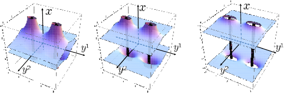
(a) $t=0$                              (b) $t=2$                              (c) $t=3$

Figure 1: The time evolution of the singular hypersurfaces $h=0$ for two equal-mass 1-branes in $D=6$ and $\Lambda>0$. Our parameters are $\Lambda=1$, $L=1$, and $M=1$. We depict the surfaces with $y^{3}=y^{4}=0$. The regular part of the spacetime corresponds to that between these hypersurfaces.

(a) $x=0$-plane                                      (b) $y_{\perp}=0$-plane

Figure 2: The contours show the level set $h=0$ at $y_{\perp}=0$ for two 1-branes in the case of $D=6$ and $\Lambda>0$. The thick solid lines correspond to the surface of the $h=0$ at the initial positive time. The lines change to solid, dashed, and then dotted ones as the time evolves. As the time progresses, the domain expands. Hence, the two level sets approach each other.

The regular spacetime with two 1-branes ends on these singular hypersurfaces. First, we consider the period of $t>0$. Initially ($t=0$), the regular region is small, but it increases in time. The $x=0$ plane is always regular. In the large-$|x|$ region, two branes are disconnected by a singularity. The metric (23) implies that the transverse dimensions ($y_{\perp}$) expand asymptotically as $\tilde{\tau}$, while the spatial dimension of the world volume ($x$) contracts asymptotically as $\tilde{\tau}^{-(D-4)/2}$ for fixed spatial coordinates ($x$ and   $y$), where $\tilde{\tau}$ is the proper time of the coordinate observer. However, it is observer-dependent. As we mentioned before, it is static near branes, and the spacetime approaches a Milne universe in the far region ($|\,\!\!\!\mbox{ \boldmath$y$}|\rightarrow\infty$), which expands in all directions isotropically. For the period of $t<0$, the behavior of spacetime is the time reversal of the period of $t>0$.

The proper distance at $x=0$ and $y_{\perp}=0$ between two branes is given by

$$d(t) = \int_{-L}^{L}dy^{1}\left[{\Lambda\over 2}t^{2}+{M\over|y^{1}+L|^{D-4}}+{M\over|y^{1}-L|^{D-4}}\right]^{1\over D-2}$$ (32)

$$= \left({ML^{2}}\right)^{1\over D-2}\int_{-1}^{1}d\eta\left[\left({\Lambda L^{D-4}\over 2M}\right)\,t^{2}+{1\over|\eta+1|^{D-4}}+{1\over|\eta-1|^{D-4}}\right]^{1\over D-2}\,,$$

which is a monotonically increasing function of $t^{2}$. We show $d(t)$ integrated numerically in Fig. 3 for the case of $D=6$.

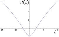
Figure 3: The proper distance between two branes at $x=0$ and $y_{\perp}=0$ for the case of $D=6$. We set $\Lambda=1$ and $M=1$. Initially ($t<0$), the distance decreases, but turns to increase at $t=0$, and then two 1-branes segregate each other.

It shows that two 1-branes are initially ($t<0$) approaching, the distance $d$ takes the minimum finite value at $t=0$, and then two 1-branes segregate each other. They will never collide (see Fig. 3).

(2) $\Lambda<0$

Next, we discuss the case of $\Lambda<0$. We illustrate the positions of two equal-mass 1-branes and time evolution of the singular hypersurface $h=0$ in Fig. 4 for the case of $D=6$. The regular part of the spacetime is the region involving those above and below the hypersurface. Two cross sections of the singular hypersurface ($x=0$ and $y_{\perp}=0$) are also shown in Fig. 5.

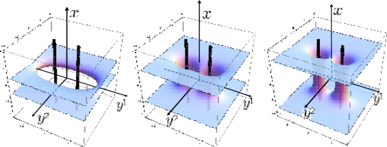
(a) $t=1$                              (b) $t=2$                              (c) $t=3$

Figure 4: The position of two equal-mass 1-branes, and the time evolution of the singular hypersurface $h=0$ with $y^{3}=y^{4}=0$ in the case of $D=6$ and $\Lambda<0$. Our parameters are $\Lambda=-1$, $L=1$, and $M=1$. The regular part of the spacetime is the region involving those above and below the hypersurface.

(a) $x=0$-plane                                      (b) $y_{\perp}=0$-plane

Figure 5: The contours show the level set $h=0$ at $x=0$ (a) and $y_{\perp}=0$ (b) for two 1-branes in the case of $D=6$ and $\Lambda<0$. The thick solid lines correspond to the surface of the $h=0$ at the initial positive time. The lines change to solid, dashed, and then dotted ones as the time evolves. The level set splits into two components, which then shrink around the two 1-branes in time.

First, we consider the period of $t\geq 0$. Initially ($t=0$), all of the region of $(D-1)$-dimensional space is regular except at $y\rightarrow\infty$ on the $x=0$ plane [see Fig. 4(a)]. As time evolves, the singular hypersurface erodes the large $x$ region as shown in Fig. 4. The   $y$-coordinate region is also invaded in time. As a result, only the region of large-$x$ and near 1-branes remains regular. When we watch this evolution on the $x=0$ plane, the singular circle appears at infinity and comes to the region of two branes [Fig. 4(a)]. A singular hypersurface eventually surrounds each 1-brane individually and then the regular regions near 1-branes splits into two isolated throats [see Figs. 4 (b), (c) and 5]. For the period of $t<0$, we find the time-reversed evolution of the case of $t>0$.

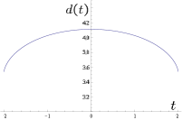
Figure 6: The proper distance between two branes at $x=0$ and $y_{\perp}=0$ for the case of $D=6$. We set $\Lambda=-1$ and $M=1$. Initially ($t<0$), the distance increases, but turns to decrease for $t>0$. A singularity appears at $t=2$ when the distance is still finite.

We also calculate the distance $d(t)$ at $x=0$ and $y_{\perp}=0$ between two branes before the singularity appears. The distance is also given by Eq. (32). However in the present case, $d$ is a monotonically decreasing function of $t^{2}$. Hence, $d$ increases when $t<0$, but it turns to decrease after $t=0$. We show the time change of the distance in Fig. 6 for the case of $D=6$. It could mimic brane collisions. However, a singularity appears between two branes before the distance vanishes, i.e., a singularity forms before collision of two branes. Hence, we cannot discuss a brane collision in this example. It is not the case if $D=3$, which we will discuss next.

II.2.2 $D=3$

Here we discuss the case of $D=3$, which may provide us a colliding 1-brane model. Although this is a toy model, it may capture the essence of brane collision. The dynamical 1-brane solution is written as

$$ds^{2} = \left[\frac{1}{2}\Lambda\left(t^{2}-x^{2}\right)+\sum_{l}M_{l}|y-y_{l}|\right]\left(-dt^{2}+dx^{2}\right)$$ (33)

$$~{}~{}~{}+\left[\frac{1}{2}\Lambda\left(t^{2}-x^{2}\right)+\sum_{l}M_{l}|y-y_{l}|\right]^{2}dy^{2},$$

where the constant $y_{l}$ denotes the position of the 1-brane with charge $M_{l}$.

Let us consider the two 1-branes with the brane charge $M_{1}$ at $y=0$ and the other $M_{2}$ at $y=L$. The proper distance between the two 1-branes is given by

$$d(t,x) = \int^{L}_{0}dy\left[\frac{1}{2}\Lambda\left(t^{2}-x^{2}\right)+M_{1}|y|+M_{2}|y-L|\right]$$ (34)

$$= \frac{1}{2}L\left[\Lambda\left(t^{2}-x^{2}\right)+\left(M_{1}+M_{2}\right)L\right].$$

Equation (34) implies that the branes collide at $t_{\rm c}(x)=\pm\sqrt{-(M_{1}+M_{2})L/\Lambda+x^{2}}$, which depends on the brane charges and the place of the world volume. On the collision, a singularity forms at $y=L/2$ due to $h=0$.

For $\Lambda<0$, the proper distance for fixed $x$ decreases as $t$ increases from $t=0$, and it eventually vanishes at $t=t_{c}$. Hence, one 1-brane approaches the other as time progresses, causing the complete collision at $t=t_{\rm c}$. If we fix the brane charges such that $M_{1}+M_{2}>0$, the branes first collide at $x=0$, and as the time evolves, the subsequent collisions occur at the larger $|x|$ [see Fig. 7(a)]. This behavior, however, changes by use of a different time coordinate. For example, if we watch the collision in the frame $T=\sqrt{t^{2}-x^{2}}$, the collision occurs simultaneously [see Fig. 7(b)].

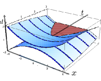
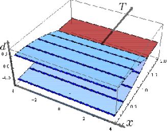
(a) $t$-coordinate                                      (b) $T$-coordinate

Figure 7: Collision of two 1-branes in three-dimensional spacetime with $\Lambda<0$. (a) The world sheets of two 1-branes are shown in the $(x,d,t)$ space, where $d(t,x)$ is the proper distance between two 1-branes at $x$. In order to see the motion of two branes, the positions of 1-branes evolved with the equal time interval are also shown by the blue (thick) curves. The 1-branes collide first at the center ($x=0$) at $t=t_{c}$ and the collision point moves to the larger-$|x|$ region. (b) The behavior of collision of two 1-branes by use of the different time $T=\sqrt{t^{2}-x^{2}}$. In this frame two 1-branes collide simultaneously.

On the other hand, when $\Lambda>0$, the proper distance with the fixed $x$ takes the minimum value

$$d_{\rm min}(x)=\frac{1}{2}L\left[-\Lambda\,x^{2}+\left(M_{1}+M_{2}\right)L\right]\,,$$ (35)

at $t=0$, if $|x|<x_{\rm max}$, where $x_{\rm max}=\sqrt{(M_{1}+M_{2})/\Lambda}$, and the distance $d$ increases as $t$ increases. For the region of $|x|>x_{\rm max}$, two branes are initially disconnected, but they are connected at $t_{c}$ as the time evolves and the distance also increases in time. Then, for $t>0$, each brane gradually separates the others as the time progresses. This is similar to the case of $\Lambda>0$ for $D>4$.

II.3 The dynamical 0-brane solution

In this section, we consider the case of $p=0$, i.e., a 2-form field strength in the action (1) in order to obtain a homogeneous cosmological solution. Since the world volume for 0-brane has only the time coordinate, the warp factor in the metric can depend on the time and transverse space coordinates.

From Eqs. (14), (17a) and (17b), we find the basic equations in the present case as

$$\partial_{t}^{2}h_{0}-\frac{4}{D-1}\Lambda=0,$$ (36a)

$$R_{ij}({\rm Y})-\frac{2}{D-1}\Lambda u_{ij}=0,$$ (36b)

$${\triangle}_{{\rm Y}}h_{1}=0.$$ (36c)

Integrating Eq. (36a) , we find

$$h_{0}(t)=\frac{2\Lambda}{D-1}t^{2}+c_{1}t+c_{2}\,,$$ (37)

where $c_{1}$ and $c_{2}$ are integration constants. Using a freedom of the time translation, we can shift $c_{1}$. $c_{2}$ is included in $h_{1}$. Hence, we can set $c_{1}=c_{2}=0$ without loss of generality, which we assume in what follows.

Equation (36b) means that the ${\rm Y}$ space is not Ricci flat due to the existence of a cosmological constant. It is different from a class of time-dependent solutions with multiple charged “singular” solutions coupled to a scalar field Maki:1992tq . The harmonic function $h_{1}$ is obtained by solving Eq. (36c). Although one can superpose the harmonic eigenfunctions to find general solution of $h_{1}$, those eigenfunctions should be solved on an Einstein space, which may not be so trivial even if ${\rm Y}$ is assumed to be a constant curvature space. Without specifying the harmonic function $h_{1}$, let us consider the dynamics of the metric in more detail.

Assuming $\Lambda>0$ and introducing a new time coordinate, $\tau$ becomes

$${\tau}=(D-2)\,t^{1\over D-2}\,,$$ (38)

and we find the $D$-dimensional metric (5) as

$$ds^{2}=\left[1+\left(\frac{\tau}{\tau_{0}}\right)^{-2(D-2)}h_{1}\right]^{-\frac{D-3}{D-2}}\left[-d\tau^{2}+\left\{1+\left(\frac{\tau}{\tau_{0}}\right)^{-2(D-2)}h_{1}\right\}\left(\frac{\tau}{\tau_{0}}\right)^{2}u_{ij}dy^{i}dy^{j}\right],$$ (39)

where $\tau_{0}=(D-2)\sqrt{(D-1)/(2\Lambda)}$. When we set $h_{1}=0$, the spacetime is an isotropic and homogeneous universe, whose scale factor is proportional to $\tau$. The $D$-dimensional spacetime becomes inhomogeneous unless $h_{1}=0$. Thus, in the limit when the terms with $h_{1}$ are negligible, which is realized in the limit $\tau\rightarrow\infty$ for $D>2$, we find a $D$-dimensional Milne universe, which is guaranteed by a scalar field with the exponential potential as we discussed in II.2. It is interesting to note that the power exponent of the scale factor is always larger than that in the matter dominated era or in the radiation dominated era.

In the case of $\Lambda<0$, time $t$ is bounded by $|t|<t_{s}$, where

$$t_{s}(y)=\sqrt{(D-1)h_{1}(y)\over 2|\Lambda|}$$ (40)

is the time when a singularity appears at $y$. Thus if we assume that $h_{1}(y)>0$, the spacetime has initially no singularity, but the Universe collapses to a big crunch, which happens at the different time $t_{s}(y)$ at each spatial point $y^{i}$.

III Conclusion

We have derived the dynamical $p$-brane solutions with a cosmological constant and discussed their applications to brane collision and cosmology. These solutions were obtained by adding a cosmological constant $\Lambda$ in the $D$-dimensional $p$-brane action Gibbons:2005rt . The basic idea was to consider field configurations in higher dimensions that are obtained by replacing the constant in supersymmetric $p$-brane solutions with warped compactifications, by a field on the world volume spacetime of the $p$-brane. The resulting $D$-dimensional metric and the $(p+2)$-form field strength depend not only on the quadratic function of the time but also on that of spatial coordinates of the world volume of the $p$-brane. We could never neglect the coordinates of world volume if we add a cosmological constant. Thus, we find that the form of $D$-dimensional metric is similar to that of the $p$-brane with a trivial or vanishing dilaton. The difference from the $p$-brane metric is that the $(D-p-1)$-dimensional transverse spacetime ${\rm Y}$ is an Einstein space and is not in general Ricci flat except for the case of the 1-branes. Moreover, the solution tells us that the function $h$ depends on all the world volume coordinates of the $p$-brane. Hence, the contribution of the field strength except for the 2-form leads to an inhomogeneous universe.

We have discussed the dynamics of 1-branes in the $D$-dimensional theory. Since the curvature for the solution is singular at the places where $h=0$, we should consider a domain where the metric is regular. In the asymptotic far-brane region, for a positive cosmological constant the 1-brane spacetime with $D>4$ approaches the $D$-dimensional Milne universe, while for a negative cosmological constant it does a conformally flat and static inhomogenenous spacetime. On the other hand, in regions close to the branes, for concreteness, we have considered the case of two branes in detail. For a positive cosmological constant, one 1-brane is approaching the other as the time evolves for $t<0$ but separates the other for $t>0$. In the case of $D>4$, for a negative cosmological constant, we have found that all of the domain between the branes are initially connected, but some region (near small $x$) shrinks as the time increases, and eventually the topology of the spacetime changes such that parts of the branes are separated by a singular region surrounding each 1-brane. Thus, in the case of $D>4$ 1-branes never collide. On the other hand, the case of $D=3$, for a negative cosmological constant and $t>0$, could provide an example of colliding branes. We found that the collision time depends on both brane charges and the place in the world volume. As we illustrated in Fig. 7, the collision process was observer-dependent.

Finally, we have also used the 0-brane solutions with a 2-form field strength and a cosmological constant to study cosmology. In the case of $D=4$, the scale factor of our four-dimensional spacetime is a linear function of the cosmic time which is the same evolution as the Milne universe. Without a cosmological constant, we get the cosmic evolution in the radiation dominated universe. Thus, although adding a cosmological constant helps to obtain the expansion law which is closer to the realistic one, it turned out that it was not still enough.

Although one might think that the examples considered here may not provide realistic cosmological models, this is inevitable in such fundamental theories like supergravities unless we also introduce more matter fields and others. However, the properties we have discovered would give a clue to investigate cosmological models in more realistic higher-dimensional cosmological settings.

References

- (1) H. Lu, S. Mukherji, C. N. Pope and K. W. Xu, Phys. Rev. D 55 (1997) 7926 [arXiv:hep-th/9610107].
- (2) H. Lu, S. Mukherji and C. N. Pope, Int. J. Mod. Phys. A 14 (1999) 4121 [arXiv:hep-th/9612224].
- (3) C. M. Chen, D. V. Gal’tsov and M. Gutperle, Phys. Rev. D 66 (2002) 024043 [arXiv:hep-th/0204071].
- (4) N. Ohta, Phys. Lett. B 558 (2003) 213 [arXiv:hep-th/0301095]; Phys. Rev. Lett. 91 (2003) 061303 [arXiv:hep-th/0303238].
- (5) G. W. Gibbons, H. Lu and C. N. Pope, Phys. Rev. Lett. 94 (2005) 131602 [arXiv:hep-th/0501117].
- (6) H. Kodama and K. Uzawa, JHEP 0507 (2005) 061 [arXiv:hep-th/0504193].
- (7) H. Kodama and K. Uzawa, JHEP 0603 (2006) 053 [arXiv:hep-th/0512104].
- (8) P. Binetruy, M. Sasaki and K. Uzawa, Phys. Rev. D 80 (2009) 026001 [arXiv:0712.3615 [hep-th]].
- (9) T. Ishino, H. Kodama and N. Ohta, Phys. Lett. B 631 (2005) 68 [arXiv:hep-th/0509173].
- (10) K. Maeda, N. Ohta, M. Tanabe and R. Wakebe, JHEP 0906 (2009) 036 [arXiv:0903.3298 [hep-th]].
- (11) K. Maeda, N. Ohta and K. Uzawa, JHEP 0906 (2009) 051 [arXiv:0903.5483 [hep-th]].
- (12) K. Maeda and M. Nozawa, Phys. Rev. D81 (2010) 044017 [arXiv:0912.2811 [hep-th]].
- (13) G. W. Gibbons and K. Maeda, Phys. Rev. Lett. 104 (2010) 131101 [arXiv:0912.2809 [gr-qc]].
- (14) K. Maeda, N. Ohta, M. Tanabe and R. Wakebe, JHEP 1004 (2010) 013 [arXiv:1001.2640 [hep-th]].
- (15) K. i. Maeda and M. Nozawa, Phys. Rev. D 81 (2010) 124038 [arXiv:1003.2849 [gr-qc]].
- (16) N. Ohta, Phys. Lett. B 403 (1997) 218 [arXiv:hep-th/9702164].
- (17) H. Nishino and E. Sezgin, Phys. Lett. B 144 (1984) 187.
- (18) A. Salam and E. Sezgin, Phys. Lett. B 147 (1984) 47.
- (19) H. Nishino and E. Sezgin, Nucl. Phys. B 278 (1986) 353.
- (20) G. W. Gibbons, R. Gueven and C. N. Pope, Phys. Lett. B 595 (2004) 498 [arXiv:hep-th/0307238].
- (21) Y. Aghababaie et al., JHEP 0309 (2003) 037 [arXiv:hep-th/0308064].
- (22) K. Maeda and H. Nishino, Phys. Lett. B 154 (1985) 358.
- (23) K. Maeda and H. Nishino, Phys. Lett. B 158 (1985) 381.
- (24) A. J. Tolley, C. P. Burgess, C. de Rham and D. Hoover, New J. Phys. 8 (2006) 324 [arXiv:hep-th/0608083].
- (25) M. Minamitsuji, N. Ohta and K. Uzawa, Phys. Rev. D 81 (2010) 126005 [arXiv:1003.5967 [hep-th]].
- (26) A. J. Tolley, C. P. Burgess, C. de Rham and D. Hoover, JHEP 0807 (2008) 075 [arXiv:0710.3769 [hep-th]].
- (27) L. J. Romans, Nucl. Phys. B 269 (1986) 691.
- (28) C. Nunez, I. Y. Park, M. Schvellinger and T. A. Tran, JHEP 0104 (2001) 025 [arXiv:hep-th/0103080].
- (29) L. Alvarez-Gaume, P. H. Ginsparg, G. W. Moore and C. Vafa, Phys. Lett. B 171 (1986) 155.
- (30) J. Polchinski, String theory (Cambridge University Press, Cambridge, United Kingdom, 1998), Vols. I-II.
- (31) C. G. Callan, E. J. Martinec, M. J. Perry and D. Friedan, Nucl. Phys. B 262 (1985) 593.
- (32) M. Cvetic, H. Lu and C. N. Pope, Phys. Rev. D 62 (2000) 064028 [arXiv:hep-th/0003286].
- (33) H. Lu, C. N. Pope, E. Sezgin and K. S. Stelle, Nucl. Phys. B 456 (1995) 669 [arXiv:hep-th/9508042].
- (34) T. Maki and K. Shiraishi, Class. Quant. Grav. 10 (1993) 2171.
- (35) J.J. Halliwell, Phys. Lett. B185 (1987) 341; J. Yokoyama and K. Maeda, Phys. Lett. B207 (1988) 31.