A hybrid steady-state magnetohydrodynamic dust-driven stellar wind model for AGB stars

Abstract

We present calculations for a magnetised hybrid wind model for Asymptotic Giant Branch (AGB) stars. The model incorporates a canonical Weber-Davis (WD) stellar wind with dust grains in the envelope of an AGB star. The resulting hybrid picture preserves traits of both types of winds. It is seen that this combination requires that the dust-parameter ($\Gamma_{d}$) be less than unity in order to achieve an outflow. The emergence of critical points in the wind changes the nature of the dust-driven outflow, simultaneously, the presence of a dust condensation radius changes the morphology of the magnetohydrodynamic (MHD) solutions for the wind. In this context, we additionally investigate the effect of having magnetic-cold spots on the equator of an AGB star and its implications for dust formation; which are seen to be consistent with previous findings.

1 Introduction

In recent years several observations of evolved stars and planetary nebulae have indicated that magnetic fields may exist in these objects (e.g. Amiri et al. 2010, Jordan et al. 2005, Herpin et al. 2006, Sabin et al. 2007a Sabin et al. 2007b and Miranda et al. 2001). The inferred magnetic fields in such objects, at the distances of the masers, indicate a variety of field strengths ranging from a few milligauss to a hundred gauss or so (Vlemmings et al., 2005; Vlemmings et al., 2006). This in turn, may indicate a variety of field strengths at the surfaces of such objects. The idea of studying the effects of a magnetic field on the nature of the AGB wind has been carried out mainly with regard to explaining the diversity of the observed shapes (see for example Chu et al. 1987 and Stanghellini et al. 1993 and references therein) of planetary nebulae. As a result, the modelling of magnetic fields in these stars has focussed on the final stages of the AGB phase, at the very tip of the AGB, or on the post-AGB phase itself, employing the so called interacting wind scenario (see Frank, 1999; Franco et al., 2001; Gardiner & Frank, 2001, for outlines of the key points of interacting wind models).

It has therefore been argued that magnetic fields play a vital role in shaping planetary nebulae by several researchers. However, it is not completely certain whether magnetic fields play a dynamic global or local role in this regard. The reader is referred to work carried out by Soker and co-workers (e.g. Soker & Kastner, 2003; Soker & Zoabi, 2002; Soker, 2002; Soker & Clayton, 1999; Soker & Harpaz, 1999; Soker, 1998) for discussion regarding this topic. Moreover, current state-of-the-art MHD models for the winds of stars at the tip of the AGB, do not take into account the effect of radiation pressure on the dust grains in the envelope of an AGB star. It is generally thought that the mass loss in AGB stars is largely governed by this mechanism coupled with strong stellar pulsations (Lamers & Cassinelli, 1999; Elitzur et al., 2003; Bowen, 1988; Bowen & Willson, 1991; Fleischer et al., 1992; Wood, 1979; Bedijn, 1988). However, to the best of our knowledge, there have not been any investigations combining a standard dust-driven wind scenario with MHD effects, in the literature. Such a study, given the importance of magnetic activity in AGB stars, would help bring together two different sub-classes of stellar winds. This is the aim of the current paper; to investigate the implications of combining magneto-rotational effects with a dust-driven wind in AGB stars. It is to be mentioned that this would be applicable at the early stages of the AGB phase, long before the interacting wind scenario becomes important, wherein the models mentioned above would be more likely candidates for describing the outflows.

At this juncture, we conduct a brief survey of the available literature with regard to both dust-driven winds and magneto-rotational equatorial winds. However, the reader is referred to a review by Tsinganos (2007, and references therein) for MHD outflows and likewise, reviews by Dorschner (2003) and Habing & Olofsson (2004) for historical reviews of AGB stars and dust-driven winds. Thereafter, the model developed in the current study, is elucidated.

With regard to magneto-rotational equatorial winds, seminal work was carried out by Weber & Davis (1967, WD). They formulated a steady state description for the radial and azimuthal components of the solar wind’s momentum. Essentially the same results were also arrived at independently, by Mestel (1967). These studies formed the groundwork upon which further studies were conducted. Thereafter, magnetic braking by a stellar wind was also investigated by Mestel (1968) and later in greater detail by Okamoto (1974, 1975), wherein the theory was extended to cover a variety of field configurations with poloidal fields. The Weber and Davis equatorial wind theory was extended by Goldreich & Julian (1970) towards a relativistic treatment of the wind, including the effects of pressure and gravitation. Michel (1969) carried out a similar analysis of the WD model but neglected pressure and gravity and thus, relativistic magnetosonic critical points do not appear in his model. The first effort to investigate the importance of the interactions between the gas and the magnetic field, with regard to determining properties of the structure and dynamics of the solar corona, was carried out by Pneuman & Kopp (1971). They found that the assumed dipolar field configuration had a profound effect on the solar wind in creating streamers. Yeh (1976) conducted a parametric study of the mass and angular momentum effluxes of magneto-rotational stellar winds and found that the mass efflux would be large, if the mass of the star was small, with a large radius, provided the stellar corona was dense and hot. Simultaneously, he found that the angular momentum efflux became greater when the magnetic field and stellar rotation parameters were increased. Belcher & MacGregor (1976) revisited the Weber and Davis theory and identified two regimes; the so-called slow and fast magnetic rotators, which are defined by the ratios of the Michel and Parker velocities of the wind. The former is related to the ratio of the magneto-rotational flux to the mass flux and the latter is related to the squares of the sound speed, escape velocity and radial bulk gas velocity at the surface. Presently, the reader is referred to Belcher & MacGregor (1976) for mathematical expressions for these quantities. Belcher and MacGregor were able to delineate the angular momentum evolution of the two types of rotators on the main sequence. Barker & Marlborough (1982) extended the Weber-Davis theory for the case of non-zero photospheric mass loss, showing that including a dimensionless constant corrected the original theory. The original WD theory was also re-analysed elsewhere, with an effort to study standing MHD shocks by Chakrabarti (1990). Various solutions of the WD solution topology were studied and he found that many of them allowed for MHD shock formation, in both accretion and winds, of a compact magnetised object. With the advent of increased computational capabilities of computers in the 1980’s, Sakurai (1985) successfully generalised the original Weber and Davis theory to two dimensions. There appear the usual slow and fast modes in his solution, as in the original Weber and Davis theory; however, in this case, the momentum equation was found to be singular on an Alfvén surface and regularising the solution on this surface alongside the boundary condition at the photosphere uniquely determined the solution of the two-dimensional problem. Keppens & Goedbloed (1999, 2000) have over the past few years, developed two- and three-dimensional MHD models for investigating magento-rotational stellar winds. Their models have clearly shown that the dipolar nature of the magnetic field structure is important for stellar winds. At the same time they have shown that the poloidal component leads to density enhancement along the equatorial region. They also find that their trans-sonic wind solutions have dead zones which have a latitudinal dependence; this can be traced back to the configuration of the magnetic field. They have also investigated shock formation in magneto-rotational outflows (Zaliznyak et al., 2003, see) and the nature and formation of Kelvin-Helmholtz instabilities (e.g. Keppens et al., 1999). These studies indicate that the mass efflux from magneto-rotational outflows can be asymmetric in nature. Their models also have been used to study the evolution of rotational velocity distribution in late-type stars while on the main sequence. The stellar winds in these stars were assumed to be WD-like steady-state winds (see Keppens et al., 1995).

Concomitant to the development of MHD winds, the field of dust-driven winds in evolved stars has flourished as a separate research focus altogether. The early models of dust-driven outflows from AGB stars were one-dimensional and did not include radiative transfer through the dust-laden envelope and dynamical dust formation (see Lamers & Cassinelli, 1999, for a brief review). Later one-dimensional models involved dynamics of dust formation and growth in a time-dependent manner building upon initial studies of C-type AGB stars (e.g. Gail & Sedlmayr, 1988; Gauger et al., 1990; Fleischer et al., 1991). These models revealed, that due to the dynamical interaction between dust and gas and the radiation field, dust-laden shells were formed in the envelopes of AGB stars (e.g Fleischer et al., 1992) and dynamical instabilities in the flow also manifested themselves leading to aspherical mass loss (see Fleischer et al., 1995; Hoefner et al., 1995; Dorfi & Hoefner, 1996). Models have also been constructed that investigate dust grain drift through the gas which modifies dust growth rates and the efficiency of the wind acceleration process (see Sandin & Höfner, 2004). There have also been further improvements in treating the radiative transfer in a frequency dependent way alongside detailed micro-physics of molecular and grain opacities (e.g. Höfner et al., 2003; Andersen et al., 2003). The reader is presently referred to a recent review by Höfner (2008) on the status of modern-day radiation-hydrodynamical modelling of dust-driven winds of AGB stars. The modelling of dust-driven winds has elsewhere, been extended to more than one dimension, capturing the aspherical nature of the outflow in a very clear way (see Woitke & Niccolini, 2005; Woitke, 2005, 2006; Woitke & Quirrenbach, 2008; Woitke, 2008). These models incorporate hydrodynamics with radiation pressure on the dust, equilibrium chemistry for the nucleation of dust in a time-dependent way, and they take into account radiative transfer in a frequency dependent manner. They were able to capture in their simulations, many of the highly dynamical aspects of the outflow, including turbulent and inhomogeneous dust formation and Rayleigh-Taylor flow instabilities that result in cloud-like structure formations in the efflux. With the help of such models it has become clear that the winds in these stars are far more complicated than simple one-dimensional (spherically symmetric) pictures and may have an impact on shaping planetary nebulae due to their asphericity (e.g. Reimers et al., 2000) or by having an impact on the superwind at the end of the AGB, as is suggested by Lagadec & Zijlstra (2008), with regard to the abundance of carbon in the envelopes of some AGB stars. The latter suggests that the effort to include complicated micro-chemistry of the dust grains, as is done in modern AGB wind models, may prove to be a key factor in resolving issues regarding the superwind in the late stages of the AGB phase. For a more thorough description of AGB envelopes and the stochastic nature of dust formation process itself, the reader is referred to Habing & Olofsson (2004) and to Dirks et al. (2008) as well as references therein.

It has also been argued that asymmetric mass loss on the AGB may result in kicks and spin being delivered to the nascent white dwarf within (see Spruit, 1998). More recently, the effect of kicks to white dwarfs has been investigated with regard to their impact on the dynamics of globular clusters and binaries (see Davis et al., 2008; Heyl, 2007a, b, 2008a, 2008b; Heyl & Penrice, 2009). These studies indicate that the study of AGB winds in relation to asphericity is rather important. In the literature, hybrid equatorial winds have only been considered for rotating hot stars (see MacGregor et al., 1992; MacGregor & Friend, 1987; Friend & MacGregor, 1984; Poe et al., 1989; Poe & Friend, 1986). MHD stellar winds for AGB stars have been simulated for a coupled disk and star system, clearly showing that magnetocentrifugal winds can occur in planetary nebulae and AGB stars, at the tip of the AGB (see Blackman et al., 2001, and references therein). Other researchers have considered a hybrid wind for AGB stars by coupling Alfvén waves with radiation pressure (see Falceta-Gonçalves & Jatenco-Pereira, 2002; Falceta-Gonçalves et al., 2006), showing that it is possible to obtain low-velocity mass efflux in supergiant cool stars through such a mechanism. A similar study has also been carried out for Wolf-Rayet stars (e.g Dos Santos et al., 1993), of course obtaining much faster winds. From the brief survey of the literature conducted above, it is evident that winds from AGB stars whether during the initial or final phases of the AGB can have asymmetries that result in aspherical mass loss either due to purely MHD effects, or due to the dynamics between the dust and gas and the radiation field. However, present day dust-driven models still do not include magneto-rotational effects, particularly when more and more observations indicate the presence of magnetic fields in these objects and the pure MHD wind models do not include the effect of dust condensation and radiation pressure in the envelopes of these stars. The aim of the current work is to investigate the implications of including magneto-rotational effects with a simplified dust-driven model in 1.5 dimensions; the azimuthal terms are determined entirely from their dependence on the radial terms (the standard WD-picture). We shall however, for the sake of simplicity, be considering a steady-state case. It is to be re-iterated that the current model may only be valid at the early phases of the AGB, long before the onset of the superwind at the end of the AGB.

We present the underlying assumptions of the model in the following section (§2). In §3 we present the numerical details, thereafter in §4 the results are presented and discussed. Finally, in §5 the paper is summarised and future avenues for development of the current model are briefly discussed.

2 The hybrid wind model

We begin with the standard picture of a WD-equatorial wind; we shall be following their definitions and general derivation closely. However, we shall be including the dust as a second fluid. As in the WD model we shall assume complete axial symmetry and the customary explicit form for the magnetic field within the equatorial plane,

$$\vec{B}=B_{r}(r)\hat{r}+B_{\phi}(r)\hat{\phi},$$ (1)

while the velocity of the gas and the dust can respectively, be written as,

$$\vec{u}=u_{r}(r)\hat{r}+u_{\phi}(r)\hat{\phi}$$ (2)

and

$$\vec{v}=v_{r}(r)\hat{r}+v_{\phi}(r)\hat{\phi}.$$ (3)

As can be seen, the velocity fields are functions of the radial distance alone. In addition, there is no time dependence, explicit or implicit, thus conforming with the steady-state assumption. Accordingly, the continuity equation for the gas and dust combined can be written as,

$$\rho ur^{2}+n_{d}m_{d}vr^{2}\Theta(r-r_{d})=\mathrm{constant},$$ (4)

where, $\rho$ is the gas density in cgs units, $n_{d}$ is the number density of the dust grains and $m_{d}$ is the mass of a single dust grain. $\Theta(r-r_{d})$ is the standard Heaviside function which is equal to unity for $r\geq r_{d}$. Prior to the dust formation radius, there is only one fluid, namely the gas. Please note that we have dropped the subscript $r$ from the radial velocities for brevity and future convenience. We are explicitly assuming, for the sake of simplicity, that all dust formation occurs at a certain distance ($r_{d}$) from the centre of the star. Beyond this, there is no further condensation of dust. We shall also assume that all the dust grains are identical and perfectly spherical, with a radius of $a=0.05\mu$m and a mass density of $\rho_{d}\approx 2.25$g/cm³ (e.g. Lamers & Cassinelli, 1999). This yields the mass for an individual dust grain; $m_{d}=\frac{4}{3}\pi a^{3}\rho_{d}$.

In addition, we shall assume that the dust-to-gas ratio in the stellar wind is given by,

$$\frac{n_{d}m_{d}}{\rho}=\delta\leq\frac{1}{200},$$ (5)

following Lamers & Cassinelli (1999), in other words, $n_{d}m_{d}\ll\rho$. The maximum value for this ratio is at the dust formation radius and it decreases monotonically thereafter. For deriving the momentum equations for the gas and the dust, our starting point is the Euler equation, one for each of the fluids. For the gas we can write,

$$(\vec{u}\cdot\vec{\nabla})\vec{u}+\frac{1}{\rho}\vec{\nabla}p+\frac{GM_{*}}{r^{2}}\hat{r}-\frac{1}{\rho c}\vec{J}\times\vec{B}-\frac{n_{d}}{\rho}\vec{f}_{D}=0,$$ (6)

where $p$ is the gas pressure and $\vec{J}$ is the current density. It is assumed here implicitly that there is no relative motion of the ions with respect to the neutrals. The first and second terms are related to the velocity and pressure gradients respectively, the third term is the gravitational acceleration on the gas, the fourth term is the Lorentz force divided by the gas density and the final term is proportional to the drag force that is experienced by the gas, due to the dust grains moving through it. Assuming force-free MHD it can be shown that (e.g. Weber & Davis, 1967)

$$r(uB_{\phi}-u_{\phi}B_{r})=\mathrm{constant}=-R_{0}^{2}\Omega B_{r,0},$$ (7)

where, $R_{0}$ is the stellar radius (radius of the photosphere), $\Omega$ is the rotation rate of the star and $B_{r,0}$ is the radial component of the magnetic field at the stellar surface.Requiring that $\vec{\nabla}\cdot\vec{B}=0$, yields the familiar relation

$$r^{2}B_{r}=R_{0}^{2}B_{r,0}.$$ (8)

Presently, let us turn our attention to the Euler equation for the second fluid, viz., the dust grains. The rationale is that obtaining expressions for the drag force components will allow us to re-write Eq. (6), the Euler equation for the gas. The Euler equation for the dust grains can be written as,

$$(\vec{v}\cdot\vec{\nabla})\vec{v}+\frac{GM_{*}}{r^{2}}\hat{r}-\frac{\pi a^{2}Q_{rp}L_{*}}{4\pi r^{2}cm_{d}}\hat{r}+\frac{1}{m_{d}}\vec{f}_{D}=0.$$ (9)

In the above equation, $Q_{rp}$ is the radiation pressure mean efficiency (e.g. Lamers & Cassinelli, 1999). In the current study, since our aim is to present a simplistic picture we shall not be calculating this term. $L_{*}$ is the luminosity of the star and $c$ is the speed of light. The first term in Eq. (9) is related to the velocity gradient of the dust grains, the second term is the gravitational acceleration experienced by the dust grain, the third term is the radiation pressure that the dust grain experiences, that drives it outward and the final term is the drag force per unit mass of the dust grain, as it moves through the surrounding gas. At this stage, we can make the usual simplifying assumption that for a single dust grain, the radiation pressure and the drag force terms in Eq. (9) dominate completely over the other terms (e.g. Lamers & Cassinelli, 1999) and balance each other. We can then write,

$$\frac{\pi a^{2}Q_{rp}L_{*}}{4\pi r^{2}cm_{d}}\hat{r}-\frac{1}{m_{d}}\vec{f}_{D}=0.$$ (10)

We can now write the radial and azimuthal components of Eq. (10) separately. Each of these components must identically vanish. Thus we get for the radial component,

$$\frac{\pi a^{2}Q_{rp}L_{*}}{4\pi r^{2}c}=f_{D}^{r},$$ (11)

where $f_{D}^{r}$ is the radial component of the drag force, defined as,

$$f_{D}^{r}=\pi a^{2}\rho(v-u)\sqrt{(v-u)^{2}+a_{th}^{2}}~{},$$ (12)

where $a_{th}$ is the thermal speed given by $a_{th}=\sqrt{2kT/\mu m_{u}}$ and $\mu m_{u}$ is the mean molecular mass of the gas. Typically for AGB stars with nearly solar abundance with pulsational shocks that extend the density structure we can use $\mu\approx 1.3$ (e.g. Bowen, 1988). From Eq. (10) we can immediately write the azimuthal momentum equation for the dust grains as,

$$\frac{f_{D}^{\phi}}{m_{d}}=0,$$ (13)

where $f_{D}^{\phi}$, the azimuthal component of the drag force, implying that there is no drag in the azimuthal direction. That is, the dust is co-rotating with the gas. Having obtained expressions for the radial and azimuthal components for the dust grains we can now re-visit the Euler equation for the gas. The radial momentum equation for the gas can be re-cast in the form,

$$u\frac{du}{dr}-\frac{u_{\phi}^{2}}{r}+\frac{1}{\rho}\frac{dp}{dr}+\frac{GM_{*}(1-\Gamma_{d})}{r^{2}}-\frac{1}{\rho c}(\vec{J}\times\vec{B})_{r}=0,$$ (14)

wherein, we have the usual definition that,

$$\Gamma_{d}=\frac{n_{d}}{\rho}\frac{\pi a^{2}Q_{rp}L_{*}}{4\pi cGM_{*}}.$$ (15)

Presently, the azimuthal momentum equation for the gas can be written, after some re-arrangement, as,

$$\rho ur^{2}\frac{d}{dr}(ru_{\phi})-r^{2}B_{r}\frac{d}{dr}(rB_{\phi})=0.$$ (16)

It is to be noted that the azimuthal component of the drag force does not appear in Eq. (16) as it vanishes (see Eq. (13)). Moreover, since the dust-to-gas ratio is small, i.e., $n_{d}m_{d}\ll\rho$ and since the dust and gas velocities are expected to be on the same order with the dust velocity exceeding the gas velocity by a reasonable fraction of the gas velocity, it is reasonable to make the approximation that $\rho ur^{2}\gg n_{d}m_{d}vr^{2}$. This allows us to further make the approximation that $\rho ur^{2}=\mathrm{constant}$ in Eq. (4). Therefore, we can immediately recover the usual expression for the total specific angular momentum of the wind as,

$$ru_{\phi}-\frac{B_{r}}{4\pi\rho u}rB_{\phi}=L=\Omega r_{A}^{2},$$ (17)

where $r_{A}$ is the Alfvén radius, defined as the distance from the centre of the star at which the radial magnetic energy density is equal to the kinetic energy density, i.e., $\frac{1}{2}\rho u^{2}=\frac{B_{r}^{2}}{8\pi}$. At this stage, we assume a polytropic equation of state for the gas as given by,

$$p=p_{0}\left(\frac{\rho}{\rho_{0}}\right)^{\gamma},$$ (18)

where, $p_{0}$ and $\rho_{0}$ are the pressure and density, respectively, at the surface of the star and $\gamma$ is the polytropic index. Then writing the density and the Lorentz force term of Eq. (14) as functions of radius and the radial velocity, we can easily obtain an expression for the gas velocity gradient as,

$$\frac{dw}{dx}=\frac{w}{x}\frac{N(w,x)}{D(w,x)}~{},$$ (19)

where, $w=u/u_{A}$ is the gas speed normalised using the Alfvén speed and $x=r/r_{A}$, is the radial distance expressed in units of the Alfvén radius. The quantities $N(w,x)$ and $D(w,x)$ are the numerator and denominator respectively and are given by,

$$N(w,x)=\left(2\gamma S_{T}(wx^{2})^{1-\gamma}-\frac{S_{G}}{x}(1-\Gamma_{d}\cdot\Theta(x-x_{d}))\right)$$

$$\times(wx^{2}-1)^{3}+~{}S_{\Omega}x^{2}(w-1)\left(1-3wx^{2}+(wx^{2}+1)w\right)$$ (20)

and

$$D(w,x)=\left(w^{2}-\gamma S_{T}(wx^{2})^{1-\gamma}\right)(wx^{2}-1)^{3}-S_{\Omega}x^{2}\times$$

$$(wx^{2})^{2}\left(\frac{1}{x^{2}}-1\right)^{2}.$$ (21)

In the above equations, the parameters $S_{T}=\frac{2kT_{A}}{m_{p}u_{A}^{2}}$, $S_{G}=\frac{GM_{*}}{r_{A}u_{A}^{2}}$ and $S_{\Omega}=\frac{\Omega^{2}r_{A}^{2}}{u_{A}^{2}}$ along with $\gamma$ uniquely determine the locations of the critical points, and hence the morphology of the family of solutions of Eq. (19). The critical points are, as usual, defined as the locations at which the both the numerator and denominator vanish, thereby keeping the right-hand side of Eq. (19) finite. The presence of the Heaviside function in Eq. (20) represents the formation of dust at the location $x=x_{d}$, the dust condensation radius in units of the Alfvén radius. The critical wind solution of Eq. (19) will yield the gas velocity profile and thereby enable determination of other dependent variables, such as the dust velocity profile (to be discussed below), the Mach number as a function of distance from the star, the azimuthal velocity of the gas, the azimuthal component of the magnetic field, the temperature profile and the density structure of the gas in the envelope of the AGB star.

As mentioned above, we can determine the dust velocity profile after having determined $u$, the gas velocity as a function of radius, with the help of Eqs. (14) and (15). This allows us to express the drift speed as (e.g. Lamers & Cassinelli (1999)),

$$(v-u)^{4}+(v-u)^{2}a_{th}^{2}-\left(\frac{Q_{rp}L_{*}}{4\pi r^{2}\rho c}\right)^{2}=0.$$ (22)

This yields the solution (after employing Eq. (19)),

$$v(r)=u(r)+\left(\frac{\sqrt{a_{th}^{4}+4\left(\frac{\Gamma_{d}GM_{*}}{\pi a^{2}n_{d}r^{2}}\right)^{2}}-a_{th}^{2}}{2}\right)^{1/2}$$ (23)

The dust grain number density $n_{d}$, can be obtained from Eq. (5). In the current study we are not solving for the dust velocity simultaneously with Eq. (19). However, since the dust-to-gas ratio is already a small number and decreases monotonically in the wind away from the star to become even smaller, we shall therefore make the simplifying assumption that $n_{d}m_{d}/\rho\approx\langle\delta\rangle$, the average dust-to-gas ratio in the wind. This essentially implies that $n_{d}$ falls off faster than $\rho$, in the wind; this is a reasonable assumption since the dust velocity is expected to exceed the gas velocity.

Finally the energy flux per second per steradian can be determined by expressing Eq. (19) as a total derivative. This yields,

$$\frac{F}{\rho ur^{2}} = \left(\frac{u^{2}}{2}+\frac{u_{\phi}^{2}}{2}+\frac{\gamma}{\gamma-1}\frac{p_{A}}{\rho_{A}}\left(\frac{\rho}{\rho_{A}}\right)^{\gamma-1}\right.$$ (24)

$$~{}~{}~{}\left.-\frac{GM_{*}(1-\Gamma_{d}\Theta(r-r_{d}))}{r}-\frac{B_{\phi}B_{r}}{4\pi\rho}\frac{\Omega r}{u}\right)\!.$$

It is immediately evident upon inspecting Eq. (24) that the Heaviside function will present a discontinuity in the flux at the dust formation radius, therefore, in order to preserve the constancy of energy flux across the dust formation interface at $r=r_{d}$, it becomes necessary to subtract a constant term to the energy flux outside the dust formation interface, such that,

$$\frac{\left.F(r)\right|_{{r=r_{d}}^{-}}}{\rho ur^{2}}=\frac{\left.F(r)\right|_{{r=r_{d}}^{+}}}{\rho ur^{2}}-\mathrm{constant}.$$ (25)

This constant is essentially the difference between the energy fluxes on either side of the dust formation radius ($r=r_{d}$) and is given by $const=GM_{*}\Gamma_{d}/r_{d}$. Such a constant term effectively redefines the gravitational potential, without altering the dynamics; i.e., its derivative vanishes, since it is a constant and thus, it does not change the solution topology of Eq. (19). Therefore we can write,

$$\frac{F(r\leq r_{d})}{\rho ur^{2}} = \left(\frac{u^{2}}{2}+\frac{u_{\phi}^{2}}{2}+\frac{\gamma}{\gamma-1}\frac{p_{A}}{\rho_{A}}\left(\frac{\rho}{\rho_{A}}\right)^{\gamma-1}\right.$$ (26)

$$~{}~{}~{}\left.-\frac{GM_{*}}{r}-\frac{B_{\phi}B_{r}}{4\pi\rho}\frac{\Omega r}{u}+\frac{GM_{*}\Gamma_{d}}{r_{d}}\right).$$

Similarly, for $r\geq r_{d}$ we obtain Eq. (24), thus we ensure that flux is constant across the dust formation interface.

This completes our derivation of the governing equations for the hybrid wind model. We see that once a solution of Eq. (19) is determined, i.e., the gas velocity profile, it in turn determines all the other relevant variables including the dust grain velocity as given by Eq. (23) and the energy fluxes given by Eqs. (24-26). In the following section we shall describe the numerical treatment breifly and the results are presented and discussed in §4.

3 Numerical details

The ordinary differential equation (ODE) for the gas velocity gradient, Eq. (19) was integrated as an initial value problem for a range of initial conditions in the $w-x$ phase space. The domain of integration was $x_{0}\leq x\leq 5$, where $x_{0}$ represents the stellar surface. Table 1 summarises all the physical parameters employed for a typical AGB star. The first step in the numerical procedure is the determination of the critical points, this is described below.

Table 1: Summary of the different parameters for modelling an AGB star hybrid wind

Parameter	Symbol	Value and/or Comment
Mass	$M$	$\sim 5M_{\odot}$
Radius	$R_{0}$	$\sim 500R_{\odot}$
Mass loss rate	$\dot{M}$	$\sim 1.6\times 10^{-6}M_{\odot}$ per year
Surface magnetic field strength	$B_{0}$	$\sim 1$ G
Bulk gas velocity (radial) at the surface	$u_{0}$	$\sim 2\times 10^{-8}v_{esc,0}$ (vanishingly small)
Surface temperature (effective)	$T_{0}$	$\sim 3000$K
Stellar rotation rate	$\Omega$	$\sim 2\times 10^{-10}$ rad/s
Surface escape velocity	$v_{esc,0}$	$6.19\times 10^{6}$ cm/s
Polytropic exponent	$\gamma$	1.06

It is to be mentioned in this regard, that we chose the value of the polytropic exponent to be approximately mid-way between unity and the values employes in current 2D-axisymmetric MHD codes, $\approx 1.13$ (e.g. Keppens & Goedbloed, 1999). A value of unity represents an insothermal equation of state and since the envelopes of AGB stars may be well-mixed due to convection, we chose a value slightly more than unity to resemble a sort of effective cooling.

3.1 Determination of critical points

The critical points are the locations in the $w-x$ phase space at which both the numerator ($N(w,x)$) and the denominator ($D(w,x)$) in Eqs. (20) and (21), identically vanish. Once the values of the parameters $S_{T}$, $S_{G}$, $S_{\Omega}$ and $\gamma$ are established, we then proceed to solve the system of non-linear algebraic equations given by,

$$N(w_{s},x_{s})=0$$ (27)

$$N(w_{f},x_{f})=0$$ (28)

$$D(w_{s},x_{s})=0$$ (29)

$$D(w_{f},x_{f})=0,$$ (30)

where, $x_{s}$ represents the distance from the photosphere (in units of $r_{A}$) at which the gas velocity is equal to the local sound speed, $w_{s}$ (in units of $u_{A}$). Similarly, the point $(w_{f},x_{f})$ represents the location in the phase space at which the kinetic energy density of the gas is equal to the local total magnetic energy density, i.e., $\frac{1}{2}\rho u^{2}=\frac{B_{r}^{2}+B_{\phi}^{2}}{8\pi}$; the so-called fast point. The root finding is accomplished using a Levenberg-Marquardt medium-scale root finding algorithm (e.g. More, 1978). Typical tolerances employed were about $10^{-15}$ in order to ascertain the zeros of the system of equations (27 - 30). This procedure is carried out for parameters $S_{T}$, $S_{G}$ and $S_{\Omega}$ on both sides of the dust formation interface. Across the interface the only change is that,

$$S_{G}^{+}=S_{G}^{-}(1-\Gamma_{d}),$$ (31)

where $S_{G}^{+}$ represents the value of the parameter outside of the dust formation interface, while $S_{G}^{-}$ represents the value inside the dust formation interface. The remaining two parameters $S_{T}$ and $S_{\Omega}$ are unchanged across the interface. Presently, we describe the procedure employed for determining the location of the radial Alfvén point and the dust parameter $\Gamma_{d}$.

3.2 Determination of the radial Alfvén point and dust parameter $\Gamma_{d}$

We begin with a set of parameters $S_{T}$, $S_{G}$ and $S_{\Omega}$ that are chosen arbitrarily; however, with the constraint that, for the given set of parameters, a critical solution is not physically possible. The rationale being that a purely Weber-Davis wind is not possible for an AGB star. This will be explained in detail later, when the results are discussed. Once the above mentioned parameters are chosen, the remaining parameters $u_{A}$ and $r_{A}$ are continuously varied for different values of $\Gamma_{d}$ until we are able to achieve a physical critical solution. The chief criterion for the latter being that the solution is continuous through the radial Alfvén point and does not have a kink and is required to originate at the base of the wind sub-sonic, pass through all three critical points, viz., the sonic point, the radial Alfvén point and the fast point and subsequently leave the star super-Alfvénic. The reader at this stage is referred to the subsection on determination of the critical solution for details (see §3.3.2). Following an initial guess for the parameters ($u_{A}$, $r_{A}$) with $\Gamma_{d}$ fixed to a certain value, they are varied with typical step sizes of $10^{-6}$ until suitable values are obtained. Once $u_{A}$ and $r_{A}$ are determined, the temperature at the radial Alfvén point is determined according to,

$$T_{A}=T_{0}\left(\frac{u_{0}R_{0}^{2}}{u_{A}r_{A}^{2}}\right)^{1-\gamma},$$ (32)

wherein, the parameters at the base of the wind (subscripted with $0$) are given in Table 1. We now turn our attention to the matter of integrating the ODE in Eq. (19) after having determined the above mentioned parameters.

3.3 Integration of the ODE and determination of the critical solution

3.3.1 ODE Integration

Integration of the ODE was accomplished with the software package ODEPACK employing the subroutine DLSODE using backward difference formulae and chord iteration with the Jacobian supplied (Hindmarsh, 1983; Brown & Hindmarsh, 1989). Initial conditions were supplied at the beginning of the integration. Typical error tolerances for convergence testing that were employed were on the order of $10^{-12}$ for both the absolute and relative errors (see Hindmarsh, 1983). For a typical integration over the domain $x_{0}\leq x\leq 5$, a step size of $10^{-8}$ was employed, resulting in typically $10^{8}$-$10^{9}$ function evaluations. A hybrid stellar wind software package was specifically developed for the current study and this was constructed to be capable of reproducing self-consistently the entire family of solutions beginning with an arbitrary choice of wind parameters. The entire code takes approximately an hour to execute on an AMD Opteron^® 844 1.8 GHz processor.

3.3.2 The critical solution

The critical solution is rather unique; it passes through all three critical points. In the current study the critical solution was determined using a tail procedure. For a given set of parameters $\gamma$, $S_{T}$, $S_{G}$ and $S_{\Omega}$, forward and backward integrations were carried out from the points $(w_{s},x_{s})$ and $(w_{f},x_{f})$. The backward integration from $(w_{s},x_{s})$ was carried out all the way to the photosphere of the star and similarly, the forward integration from $(w_{f},x_{f})$ was carried out all the way to the outer boundary of the domain at $x=5$. In between the backward integration from $(w_{f},x_{f})$ was matched with the forward integration from $(w_{s},x_{s})$. An initial guess was made for the matching point to be half way between $x_{s}$ and $x_{f}$ defined by $x_{m}$. The tails of the forward and backward integrations were terminated at this location and the values of the gas velocity $w$ and the velocity gradient $\frac{dw}{dx}$ were compared for the two tails to ensure that the conditions

$$\left|\left(\Delta w=\left.w(x_{m})\right|_{{x=x_{m}}^{-}}-\left.w(x_{m})\right|_{{x=x_{m}}^{+}}\right)\right| \leq 10^{-7}$$ (33)

$$\left|\left(\left.\frac{dw}{dx}\right|_{{x=x_{m}}^{-}}-\left.\frac{dw}{dx}\right|_{{x=x_{m}}^{+}}\right)\right| \leq 10^{-7},$$ (34)

were both met. If the conditions in Eqs.(33) and (34) were not met, then depending upon the sign of $\Delta w$, the matching point $x_{m}$ was appropriately shifted either forward or backward by a small amount, typically by $\Delta x_{m}=10^{-6}$ and the tail procedure was re-iterated. Once the tail procedure was successful the critical solution was considered to be determined. This ensured that the critical solution was continuous through the radial Alfvén point. The tolerance employed in Eqs. (33) and (34) was considered to be sufficient given the fact that the integration step size was $\Delta x=10^{-8}$. For achieving a higher tolerance, a further reduction in the step size was found to be necessary, rendering the the procedure needlessly lengthy and increasingly cumbersome in a computational sense.

This completes our discussion of the numerical details regarding determining the complete family of solutions of Eq. (19). The results are presented in the following section and are discussed therein.

4 Results and Discussion

We present the results obtained by integrating the ODE in Eq. (19) to obtain the family of solutions. In the current study, the following methodology was employed for calculating the hybrid wind. First, for a certain set of arbitrary parameters {$S_{T}$, $S_{G}$, $S_{\Omega}$ and $\gamma$}, Eqs. (27-30) were solved to obtain the location of the slow and fast points, with the radial Alfvén point located at $(1,1)$ in the $w-x$ phase space. At this stage, the dust parameter $\Gamma_{d}$ was set equal to zero, meaning that there hasn’t been any dust formation in the gas. The parameters are chosen such that a pure WD wind is not a physical one, i.e., it is not continuous through the radial Alfvén point (see Figure 3 and discussion thereof). The rationale being that for AGB stars, it is not possible to have a mass efflux without dust formation in the envelope, therefore a pure WD wind is explicitly required to not be a physical solution. Second, the dust parameter was set equal to a fraction such that $0\leq\Gamma_{d}\leq 1$ and the procedure described in §3.2 for determing the Alfvén velocity and radius is carried out in tandem with solving Eqs. (27-30) to obtain the sonic point and the fast point. Each time this yields a set of parameters {$u_{A}$, $r_{A}$, $(w_{s},x_{s})$, $(w_{f},x_{f})$}. With these parameters, Eq. (19) is integrated to obtain the critical solution according to the procedure described in §3.3.2. If success is achieved in finding the critical solution then the iterations are ceased and the resulting parameters are fixed for the given value of $\Gamma_{d}$.

We then determine the temperature profile using the velocity profile of the critical solution. This is achieved using the prescription,

$$T(r)=T_{A}\left(\frac{u_{A}r_{A}^{2}}{ur^{2}}\right)^{\gamma-1},$$ (35)

where, $T_{A}$ is the Alfvén temperature and is given by Eq. (32). Once the temperature profile is known, it is possible to invert Eq. (35) to yield the radius $r_{d}$, at which the temperature falls below the dust condensation temperature $T_{d}$. Once the dust condensation radius ($r_{d}$) is determined, we then proceed to determine the family of solutions to Eq. (19) such that integration from the photoshpere at $r=R_{0}$ to $r=r_{d}$ is carried out with $\Gamma_{d}=0$ and integration from $r=r_{d}$ to the outer boundary at $r=5r_{A}$ is done with $\Gamma_{d}\neq 0$. The same is then done for the critical solution as well.

As mentioned before, it is implicitly assumed, for the sake of analysing a patently simple model, that beyond the dust condensation radius the value of $\Gamma_{d}$ is constant. Concordantly, all the dust forms at the condensation radius and the dust-to-gas ratio is small and given by Eq. (5). The family of solutions determined using the procedures described above are shown in Figure 1. For the solutions shown therein, the dust parameter was fixed at $\Gamma_{d}=0.3$.

Figure 1: Family of solutions of Eq. (19) with parameters $u_{A}\approx 0.09v_{esc,0}$, $r_{A}\approx 63.93R_{0}$, $\Gamma_{d}=0.3$ and remaining parameters as given in Table 1. The dashed line at $r\approx 8.65R_{0}$ represents the dust formation radius.

Figure 2: Illustration showing the locations of the different types of solutions of Eq. (19)

It can be seen that the dust condensation radius is located at $r_{d}\approx 8.65R_{0}$. The temperature at this location was determined using Eq. (35), to be approximately $1200$K. The dust condensation temperature was chosen somewhat arbitrarily to lie between $1000-1500$K. Within the dust condensation radius $x_{d}$, the wind solution to Eq. (19) is a purely Weber-Davis-type of wind, and thereafter it is a hybrid wind with dust grains included. The topology of solutions in Figure 1 looks typically like a WD-solution, with the three critical points clearly visible, viz., the sonic point, the radial Alfvén point and the fast point. The critical solution emerges from the surface of the star sub-sonic, gets accelerated through to the dust condensation radius, subsequently passes through the three critical points and finally emerges super-Alfvénic at large distances.

At this stage it is convenient to classify the different types of solutions in Figure 1. The different types of solutions and their respective locations in the phase space are illustrated qualitatively in Figure 2. Therein, it can be seen that the unphysical double-valued solutions to the left of the sonic point are referred to, in the current study, as Type I solutions. The failed wind solutions, directly below the sonic point, are called Type II. The unphysical multi-valued solutions that make loops, between the radial Alfvén point and the fast point, are designated as Type IIIa. The unphysical double-valued solutions adjacent to the loop solutions are called Type IIIb.

The solitary unphysical solution that passes through the sonic X-type singularity, is called the Bondi solution, this is labelled as $B$, in Figure 2. While the unphysical double-valued solution that intersects the critical solution, at exactly the two Alfvén points, is designated the Alfvénic solution; labelled $A$. Similarly, the critical solution is labelled as $C$.

The unphysical wind solutions that start at the photophere with super-sonic velocities, just to the right of the Bondi solution and subsequently pass through the radial Alfvén point and get decelerated to sub-sonic velocities at large distances from the star, are designated as Type IVa. Meanwhile, the unphysical double-valued solutions that pass through the radial Alfvén point alone, are designated as Type IVb. Finally, the unphysical double-valued solutions, in the region between the critical solution and the Alfvénic solution, immediately to the right of the fast point, are referred to as Type V.

As mentioned earlier, the dust grains condense from the gas beyond $r_{d}$, where the temperature falls below the condensation temperature. Beyond $r_{d}$, we threfore solve the hybrid ODE with a fixed value of $\Gamma_{d}$. Thus at the dust condensation radius, the two types of solutions, dust-free and hybrid, must match, in terms of velocity of the gas. This is illustrated in Figure 3, where we have expressed the coordinates using a logarithmic scale to facilitate examination.

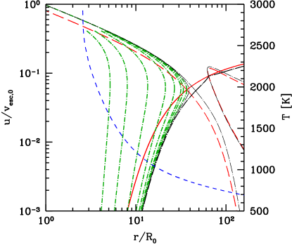
Figure 3: Plausible hybrid wind solutions with parameters $u_{A}\approx 0.09v_{esc,0}$, $r_{A}\approx 63.93R_{0}$, $\Gamma_{d}=0.3$ and remaining parameters as given in Table 1. The red solid line and black long-dash-dotted line intersecting at the radial Alfvén point, are the critical solutions of the hybrid wind model and pure WD wind model, respectively. The green-short-dash-dotted lines are possible Type I wind solutions of a pure WD wind that can leave the star via the hybrid critical solution after dust condensation at the intersection points of the green-short-dash-dotted lines and the red solid line. The blue dashed line is the temperature profile calculated for the hybrid wind critical solution. It should be interpreted using the secondary axis.

In Figure 3, the red solid line represents a hybrid wind solution for a dust parameter of $\Gamma_{d}=0.3$, while the black long-dash-dotted line that passes through the radial Alfvén point with a kink at $(u_{A},r_{A})$, is a pure WD solution with $\Gamma_{d}=0$. As can be clearly seen, the kink at the radial Alfvén point indicates that this solution is not physical. This indicates that it is not possible to have a pure WD wind for AGB stars; only with dust formation is it possible to achieve an outflow. The Bondi type solutions for both the hybrid wind (long-dashed red line) and the pure WD solution (black long-dash-dotted line), can also be seen to pass through the respective sonic points. Similarly the two fast points can also be distinguished clearly for the two types of solutions; the Alfvénic solutions pass through them. It is to be mentioned at this juncture, that inclusion of an outward force in the wind due to radiation pressure has the effect of suppressing both the sonic point and the fast point towards the photosphere; the sonic and the fast points for the hybrid wind (in red) can clearly be seen to lie inside their respective counterparts of the pure WD wind, in terms of distance from the star’s photosphere. The green short-dash-dotted lines are solutions of Type I, for a pure WD wind. The points of intersection of the red solid line representing the critical solution of the hybrid model and the green short-dash-dotted lines, represent different dust formation radii. The temperatures corresponding to these can be inferred using the blue line, which represents the temperature profile, determined using the critical solution of the hybrid wind, via Eq. (35). Thus, if a wind solution starts off at the base of the wind sub-sonic and travels through the envelope of the AGB star according to (say) the fourth green short-dash-dotted line from the left, then it can pass through the dust formation radius at approximately $1000$K, just ahead of about $10R_{0}$ and leave the star via the red solid line, the critical solution of the hybrid wind. We therefore see that the unphysical Type I solutions that start off dust-free, can intersect the hybrid critical solution and leave the star as a hybrid critical wind. However, there is a constraint. The last Type I solution that can leave the star as a hybrid wind intersects the critical solution in red, at the sonic point. Any solution of Type I that intersects the red solid line, after it has turned and become double-valued, does not represent a physical hybrid wind. This is illustrated in the black long-dash-dotted Type I solution that turns and then intersects the red solid line, just ahead of the hybrid sonic point in Figure 3. Therefore, all the green short-dash-dotted lines are allowed possible solutions of different hybrid winds.

Figure 3 also shows that if a hybrid wind is to be achieved, there are two possibile scenarios. First, the dust formation radius can lie within or at most upon the sonic point of the hybrid wind solution. Second, it can lie beyond or upon the fast point of the hybrid solution, or exactly at the radial Alfvén point. Only the first possibility places the dust formation temperature in the acceptable range for typical AGB parameters so we will focus mainly on this class of solutions (however, c.f. Figure 9 and discussion thereof). While the latter scenarios do represent legitimate mathematical solutions, it is however unlikely that the dust formation temperature be significantly lower than about $1000$K and concomitantly, that the dust formation radius in AGB stars, should lie as far out as nearly $70R_{0}$. Since it is expected that the dust formation must occur within a few stellar radii in AGB stars, the only plausible solutions are therefore the Type I green short-dash-dotted lines, that intersect the hybrid critical line in red.

For the hybrid critical solution shown in Figures 1 and 3, it is possible to calculate the azimuthal velocity profile of the gas by manipulating Eq. (17). This is carried out and is shown in Figure 4. As can be seen the gas velocity profile rises sharply to a maximum value close to the sonic point and then falls off less steeply than the rise; this is consistent with the usual WD-picture.

Figure 4: Critical azimuthal gas velocity as a function of radius. The vertical dotted lines indicate the locations of the dust formation radius and the the three critical points.

The locations of the dust formation radius and the three critical points are also indicated therein.

In Figure 5 we have plotted the energy flux per second per steradian leaving the star, in the equatorial plane, for the critical solution, alongside the various components of the energy flux.

Figure 5: Plot showing the energy fluxes calculated using Eqs. (24-26) for the critical hybrid wind solution with parameters $u_{A}\approx 0.09v_{esc,0}$, $r_{A}\approx 63.93R_{0}$, $\Gamma_{d}=0.3$ and remaining parameters as given in Table 1. The vertical dotted lines indicate the dust formation radius and the the three critical points. The solid horizontal line represents the total constant energy flux. From the top short-dash-dotted curve shows the magneto-rotational energy, the long-dash-dotted curve represents the enthalpy, the short-dashed curve shows the variation in kinetic energy and finally at the bottom the long-dashed line represents the gravitational potential energy of the gas.

The solid line shows the total energy flux in the gas as function of radius; it is constant for the critical solution. It is the sum of all the other lines on the plot. This is calculated via Eqs. (24-26). The short-dash-dotted line is the magneto-rotational energy flux, which is the sum of the last two terms in Eq. (24). As the distance from the photosphere increases, the radial magnetic field falls of as $\sim 1/r^{2}$, however the rotational energy is expected to peak close to the sonic point, as can be inferred from Figure 4, where the azimuthal velocity peaks. The two competing terms collectively yield a large positive sum closer to the star, and the contribution diminishes quite rapidly, beyond approximately the dust formation radius, as can be seen in Figure 5. The long-dashed line represents the gravitational potential energy of the wind, the third term in Eq. (24) and it is therefore negative. The short-dashed line is the kinetic energy of the wind (the first term in Eq. (24)) which gradually increases away from the star as the wind is accelerated. On the other hand, the long-dash-dotted line is the enthalpy (the second term in Eq. (24)) which gradually decreases from a maximum value at the stellar surface where the density of the gas is expected to be the highest and follows a power law, of the form $\sim\rho^{\gamma-1}$. The decrease is quite gradual as the exponent is $0.06$ since we used $\gamma=1.06$. The contribution of the kinetic energy and the enthalpy are quite small in comparison to the magneto-rotational energy. However, when the magneto-rotational energy is added to the gravitational potential energy, then the sum is comparable to the kinetic energy. Again, the dust formation radius and the three critical points are indicated in the figure. It is also to be mentioned that, since it is possible to recover the momentum terms of Eq. (14) by differentiating Eq. (24), therefore the slopes of the different lines shown in Figure 5 would indicate the contributions of these terms. In particular, it can be clearly seen that the slopes of the magneto-rotational energy and the gravitational energy (which includes radiation pressure) are the most prominent features in Figure 5. This indicates that the the most significant contributions to accelerating the wind are indeed due to the Lorentz force term plus rotational term in Eq. (14) and the gravitational potential which includes the effect of radiation pressure on the dust grains. In this regard, it is evident upon inspecting Figure 5, that beyond approximately the radial Alfvén point, the gravitational energy flux becomes flat, indicating that the acceleration due to the gravitational potential modified by radiation pressure, becomes negligible in the wind. However, beyond $r=r_{A}$, the magneto-rotational energy still has a small contribution and continues to accelerate the wind. In summary, at small distances, ($r<\approx r_{s}$), both the magneto-rotational terms and the modified gravitational potential terms of Eq. (14) have a combined and pronounced effect in accelerating the wind; however, at large distances ($r>\approx r_{A}$) the effect of the gravitational potential becomes negligible while there still persists a small contribution from the magneto-rotational term, that mildly accelerates the wind outward.

Figure 6 shows the velocity profiles of the dust and the gas plotted as a function of distance from the centre of the star.

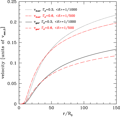
Figure 6: Dust and gas velocity profiles for two hybrid winds with parameters $u_{A}\approx 0.09v_{esc,0}$, $r_{A}\approx 63.93R_{0}$, $\Gamma_{d}=0.3$ (in black) and with parameters $u_{A}\approx 0.07v_{esc,0}$, $r_{A}\approx 53.05R_{0}$, $\Gamma_{d}=0.6$ (in red). In the former case, the dust-to-gas ratio was $\langle\delta\rangle=1/1000$ and in the latter case it was double this value, i.e. $\langle\delta\rangle=1/500$. The remaining wind parameters are given in Table 1. The dust velocity profile in each case is determined using Eq. (23).

The velocity of the dust grains exceeds that of the gas bulk, as is required by the hybrid wind model, in order to produce an outward drag force on the gas, to accelerate it outward. The velocity of the dust grains is determined according to Eq. (23), once the velocity profile of the gas is ascertained, with an assumed average value for the dust-to-gas ratio $\langle\delta\rangle$. Figure 6 shows the gas and dust velocity profiles for two different sets of model parameters. The solid black line represents the gas velocity while the dotted black line represents the corresponding dust velocity. This model had parameters $\Gamma_{d}=0.3$ and $\langle\delta\rangle=1/1000$. In order to investigate the effect of changing the average dust-to-gas ratio, we kept all other parameters of the model fixed, in particular, the radiation pressure mean efficiency and the stellar luminosity, were kept constant. Then, according to Eq. (15), if the average dust-to-gas ratio is doubled then, then accordingly, the dust parameter $\Gamma_{d}$ must also double. Thus, for the second model’s results shown in Figure 6, we took $\Gamma_{d}=0.6$ and $\langle\delta\rangle=1/500$. Thus, the red-dashed line represents the gas velocity profile, while the red-long-dash-dotted line represents the corresponding dust velocity profile. However, changing the dust parameter also changes the locations of the the three critical points. With $\Gamma_{d}=0.3$ the Alfvén velocity and Alfvén radius were found to be $u_{A}\approx 0.09v_{esc,0}$, $r_{A}\approx 63.93R_{0}$, while for $\Gamma_{d}=0.6$, the corresponding values were found to be $u_{A}\approx 0.08v_{esc,0}$, $r_{A}\approx 53.05R_{0}$ respectively. It can clearly be seen that within about $50R_{0}$ (which is approximately the location of the radial Alfvén point for the second model), the dust in the second model (red-long-dash-dotted line) has a steeper rise, indicating a larger acceleration in the wind. Beyond about $50R_{0}$, the acceleration of the wind in the second model ($\Gamma_{d}=0.6$) starts to decline (see Figure 5 and discussion thereof). However, the wind in the first model ($\Gamma_{d}=0.3$) at this distance, is still getting accelerated, therefore it’s velocity increases. Thus, when $\Gamma_{d}$ is smaller, acceleration due to radiation pressure continues to have an effect, out to larger distances from the star. In addition, at a distance of about $50R_{0}$, the temperature in the wind is about $\approx 800K$ for the model with $\Gamma_{d}=0.3$ and about $\approx 550K$ for the model with $\Gamma_{d}=0.6$. Thus, the bulk of the gas is much cooler in the latter case. As a result, it is natural that the velocities in the second model are slightly lower than the first. That being said, it is to be acknowledged that by increasing the dust parameter by increasing the average dust-to-gas ratio, the wind gets accelerated much faster closer to the star. This is expected; however, the terminal velocity in this case is lower, as the acceleration due to radiation pressure does not have a pronounced effect out to large distances ($r>\approx r_{A}$).

At this stage we turn our attention to the question of changing the temperature at the base of the wind. In AGB stars, it is likely that due to density pulsations within the star, the temperature and density at the stellar photosphere are likely to undergo change (e.g. Lamers & Cassinelli, 1999). It has also been suggested by Soker & Clayton (1999) that magnetic-cool spots probably exist in the region around the equator of an AGB star, much like our sun. If such is the case, then the temperature at the base of the hybrid wind will change locally, and this will have an effect on the stellar wind beyond the photosphere in the AGB envelope. In order to investigate this, we constructed a hybrid model with an altogether different base temperature. Following Soker & Clayton (1999), we set the base temperature in a magnetic-cool spot to be significantly less than the prescribed average $3000$K, of the stellar photosphere. Accordingly, in order to achieve a hybrid stellar wind, that starts with negligible velocity at the stellar surface and gets accelerated to super-Alfvénic velocities having passed through the dust formation radius and the the three critical points, we treated $\Gamma_{d}$, $u_{A}$ and $r_{A}$ as free parameters. As described in §3.2 we varied the values of these parameters until a successful critical solution was achieved. When the base temperature is changed to $2000$K, we found that in order to achieve a hybrid stellar wind, the three free parameters required to take on values; $\Gamma_{d}\approx 0.62$, $u_{A}\approx 0.07v_{esc,0}$ and $r_{A}\approx 52.19R_{0}$. Figure 7 shows how the morphology of the solution changes when the base temperature is changed. We have merely shown the key solutions, namely, the critical solutions, the Bondi and the Alfvénic solutions.

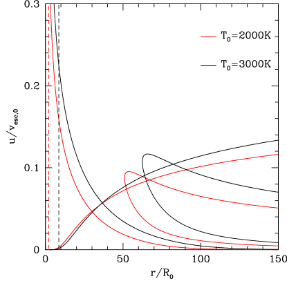
Figure 7: Plot showing the effect of changing the temperature at the base of the stellar wind. The black lines are for a hybrid wind with parameters $T_{0}=3000$K, $u_{A}\approx 0.09v_{esc,0}$, $r_{A}\approx 63.93R_{0}$ and $\Gamma_{d}=0.3$ while the red lines are for a hybrid wind with parameters $T_{0}=2000$K, $u_{A}\approx 0.07v_{esc,0}$, $r_{A}\approx 52.19R_{0}$ and $\Gamma_{d}\approx 0.62$. Both winds have identical remaining wind parameters, as given in Table 1. The dashed lines represent the locations of the respective dust formation radii for the two hybrid winds with $T_{d}\approx 1200$K, in both cases. Dust formation occurs closer to the stellar surface when the base temperature is lowered.

The solid black lines are the hybrid wind solutions when the base temperature is $T_{0}=3000$K and the dust parameter is $\Gamma_{d}=0.3$. The lighter red lines are for $T_{0}=2000$K and $\Gamma_{d}\approx 0.62$. The dashed lines at the far left indicate the locations of the respective dust formation radii for the two models; in both cases the dust formation temperature was taken to be $T_{d}\approx 1200$K. It can be clearly seen in Figure 7, that when the base temperature is decreased to $2000$K, all the critical points as well as the dust formation radius, are suppressed towards the photosphere. The formation of dust closer to the stellar surface is directly related to the steep drop in the temperature profile ahead of the photosphere in the AGB envelope. This finding is consistent with the results of Soker & Clayton (1999), who found that dust formation occurred closer to the stellar surface ahead of magnetic-cool spots on the equator of an AGB star. Additionally, the stellar wind critical solution for $T_{0}=2000$K has a lower terminal velocity than its counterpart for $T_{0}=3000$K. This is directly related to the fact that the bulk of the gas is much cooler when the base temperature is lower. If there exist magnetic-cool spots on the surface of an AGB star, then the stellar wind properties, namely the wind speed and momentum of the outflow will change, ahead of the cool spot in the envelope of the star. This will result in asymmetric flows between different parts of the star, in addition to the fact, that dust formation will occur closer to the star. These will directly lead to MHD instabilities, that can grow and become unstable and result in asymmetric mass loss. However, it is to be noted, that investigating such effects is beyond the scope of the current study. In order to investigate instabilities it will be necessary to carry out MHD calculation in at least two, if not three dimensions. By definition, the current steady-state model cannot incorporate dynamic effects such as instabilities. Addition of effects of radiative transfer, along with internal chemistry, that affects dust grain formation, with relaxation of the assumption of spherical grains, would be the ultimate goal of such an endeavour. It has already been shown by Woitke & Niccolini (2005) using 2-D hydrodynamic codes with radiative transfer, that it is possible to capture hydrodynamic instabilities. The addition of magneto-rotational effects to these models would result in richer gas (and dust) dynamics and quite different instabilities in the flow altogether, due to the presence of MHD effects. The presence of instabilities in the outflow are the precursors for asymmetric mass loss, which has been theorised to be responsible for white dwarf kicks (see Spruit, 1998; Davis et al., 2008; Heyl, 2007a, b, 2008b, 2008a; Heyl & Penrice, 2009). In this context, the current work is relevant, as it presents a steady-state solution that 2- and 3-D MHD-dust-driven wind models can reproduce by eliminating the time dependence, i.e., setting the $\partial/\partial t$ terms to zero. It also presents an additional avenue for the formation of instabilities, in AGB stellar winds.

It is also to be noted that, when the dust parameter was increased to values closer to unity, it resulted in the critical points being suppressed towards the photosphere; this can clearly be seen in Figure 7. Concordantly, as the dust parameter is increased, it results in dust condensation closer to the stellar surface. In Figure 8 we have plotted the location of the three critical points as a function of the dust parameter $\Gamma_{d}$. The short-dash-dotted line represents the location of the sonic point ($r_{s}$) as $\Gamma_{d}$ is varied, the solid line shows the variation in the radial Alfvén point ($r_{A}$), while the long-dash-dotted line shows the change in the fast point ($r_{f}$). Also plotted therein, is the temperature at the radial Alfvén point; the short-dashed line. As can be clearly seen, in the limit of $\Gamma_{d}\rightarrow 1$, the three critical points converge and their locations approach the stellar surface. The sharp decline in the radial Alfvén temperature beyond $\Gamma_{d}\approx 0.7$ indicates that the temperature profile in the AGB envelope falls off in an extremely steep manner, making the solutions of the gas momentum equation implausible and indeed unphysical.

Figure 8: Plot showing the effect of changing the dust parameter $\Gamma_{d}$ on the morphology of the family of solutions to Eq. (19). In all calculations the common parameters for the models are shown in Table 1. The short-dash-dotted line shows variation in the sonic point ($r_{s}$) as a function of $\Gamma_{d}$, the solid line shows the change in the radial Alfvén point ($r_{A}$) with changing $\Gamma_{d}$, while the long-dash-dotted line represents the change in the fast point ($r_{f}$) for the same case. The short-dashed line traces the dependence of the temperature at the radial Alfvén point on $\Gamma_{d}$, this should be interpreted using the secondary axis.

To determine the dependence of the critical points on the dust parameter, we continuously changed the value of $\Gamma_{d}$ with a step size of $10^{-4}$, within the limits shown in Figure 7 and for each given value of $\Gamma_{d}$, we determined the appropriate set of parameters {$u_{A}$, $r_{A}$, $(w_{s},x_{s})$ and $(w_{f},x_{f})$}, that yielded a continuous monotonically increasing critical solution through the critical points. Following which, the temperature at the radial Alfvén point was determined according to Eq. (32).

In simple isothermal dust-driven wind models, a stellar outflow is achieved by setting $\Gamma_{d}>1$ (e.g. Lamers & Cassinelli (1999)). This is done to counteract the force of gravity and to drive the gas outward. However, in the current study we found that setting the dust parameter to be greater than unity, did not yield a set of critical points; i.e., they were found not to exist in the domain $R_{0}\leq r\leq 150R_{0}$, for which Eqs. (27-30) were satisfied simultaneously. Hybrid winds were successfully achieved for $0<\Gamma_{d}<1$. Indeed, as is shown in Figure 7, $\Gamma_{d}\approx 0.7$ is a reasonable physical upper limit, where $T_{A}(\Gamma_{d}\approx 0.7)\approx 450$K and after which point the decline in the temperature proceeds very rapidly. It is to be mentioned that for all of the calculations carried out to produce Figure 7, the temperature at the base of the wind was $T_{0}=3000$K and all the remaining parameters were identical to those given in Table 1.

Finally, for the sake of completeness, we have shown in Figure 9, the plausible hybrid wind solutions, should the dust formation radius exist outside the fast point. Again the parameters of the hybrid wind are identical to those shown in Table 1.

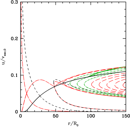
Figure 9: Plausible hybrid wind solutions with dust formation occurring beyond the fast point. The red-long-dash-dotted line and the black solid line intersecting at the radial Alfvén point, are the critical solutions of the hybrid wind model and pure WD wind model, respectively. The green-short-dash-dotted lines are possible Type V wind solutions of a hybrid wind ($\Gamma_{d}=0.3$) that can leave the star as a dust laden wind after dust formation occurs at the intersections with the solid black WD critical solution. The thick green solid line represents a possible hybrid wind solution with $\Gamma_{d}=2$.

It is to be mentioned that it is likely that dust formation lies within a few stellar radii (e.g. Lamers & Cassinelli, 1999); however, since the parameters of Table 1 may all be scalable to suit an altogether different type of star, we have therefore included Figure 9, to complete the scenario of dust forming in the envelope or indeed the outer atmosphere of the star.

In Figure 9, the solid black line represents the critical solution of a pure Weber-Davis stellar wind, without any dust. While the long-dash-dotted red line represents the hybrid wind critical solution with $\Gamma_{d}=0.3$ and $u_{A}\approx 0.07v_{esc,0}$ and $r_{A}\approx 48.20R_{0}$, the pure WD wind has the same values for $u_{A}$ and $r_{A}$. As can be seen in this case, the hybrid wind is not a physical possibility as it is not continuous through the radial Alfvén point. On the other hand the pure WD-equatorial wind is continuous. The Bondi and Alfvénic solutions for the two types of solutions, with and without dust, are also plotted in long-dash-dotted-red and black-dashed lines respectively. The long-dashed lines in red represent the hybrid unphysical solutions of Type V. The intersections of the pure WD critical solution in black, with the Type V hybrid green-short-dash-dotted lines, represent possible locations for the dust formation radius. Thus a wind may start off as a pure WD wind at the surface of the star, pass through all three critical points and then undergo dust formation beyond the fast point. At this stage the critical solution may leave the star by following a hybrid solution represented by the short-dash-dotted lines in green, after dust condensation. The red-long-dashed lines are not plausible as they have either turned and become double-valued (the left most long-dashed-red dashed line) or they do not intersect the solid black line (the long-dashed-red lines to the right of the green-short-dash-dotted lines), at least within the domain indicated. The thick solid green line that intersects the solid black line at about $r\approx 95R_{0}$, is a hybrid wind solution of Type V. This solution has the dust parameter set to a value greater than unity ($\Gamma_{d}=2$). Thus it can be seen that it is possible to have a hybrid wind with $\Gamma_{d}>1$ if $r_{d}>r_{f}$. In this case, the critical points for the hybrid wind parameters are unphysical and do not lie within the domain $R_{0}\leq r\leq 150R_{0}$ (see earlier discussion relating to Figure 8). However in this case, the critical wind solution has already been accelerated through the physically possible pure-WD critical points before dust condensation occurs in the wind. Thus, the hybrid picture can still work with the dust parameter greater than unity as long as dust condensation occurs beyond the fast point. As mentioned before, Figure 9 does not apply to AGB stars (since dust condensation likely occurs within a few stellar radii), it is included here for the sake of completeness and understanding the full nature of the hybrid wind solutions.

This completes our discussion of the results of the study. In the following section we present our summary and conclusions along side a short discussion of directions for further investigation.

5 Conclusion

We present below a brief summary of the paper and thereafter a short discussion of possible avenues for further work.

5.1 Summary

In the preceding discussion we presented a hybrid wind model for AGB stars. The model consists of incorporating a dust-driven wind with a Weber-Davis MHD equatorial wind. The resulting wind momentum equations yielded expressions for the radial and azimuthal velocities of the gas and the dust. After eliminating the azimuthal equations, two radial equations remained in the model that described the velocity profiles of both the gas and the dust. In the model described in this paper, we explicitly assumed a steady-state for the wind dynamics.

A WD wind was assumed to begin at the surface of the star, one that would eventually fail if not for the formation of dust grains at a given radius, which allows the hybrid wind to leave the star at super-Alfvénic velocities. The dust formation was assumed to occur abruptly, at a pre-determined radius. All the dust grains were assumed to be perfectly spherical with identical size. It was implicitly assumed that radiation pressure was purely in the radial direction without scattering. The opacity of the grains was implicitly assumed to be such that all of the radiation impinging on the grains was absorbed and imparted momentum to the grains. The resulting drag force was assumed to be purely radial as well. The rationale was to develop a simple model to delineate the key points of the theory.

The hybrid wind ODE was subsequently solved using finite difference methods, for different values of the dust parameter $\Gamma_{d}$. It was found that, in order to achieve a successful hybrid wind, it was necessary for the dust parameter to take values such that $0<\Gamma_{d}<1$, when dust formation occurs within the slow point, i.e., $r_{d}<r_{s}$. The effect of changing the dust parameter revealed that $\Gamma_{d}>1$, did not yield plausible stellar wind parameters. It was found that when $\Gamma_{d}\rightarrow 1$, all three critical points converged to the the stellar surface.

Finally, the effect of changing the temperature at the base of wind was also investigated. The temperature was changed from $T_{0}=3000$K to $T_{0}=2000$K to represent a magnetic-cold spot on the equator of an AGB star. It was found that lowering the temperature not only changed the morphology of the family of solutions by suppressing the critical points towards the stellar surface, but also required a greater value of the dust parameter in order to achieve a successful hybrid wind. This additionally resulted in suppressing the dust formation radius as well, towards the photosphere of the star, consistent with the findings of Soker & Clayton (1999). Since the velocity of the wind, ahead of the magnetic-cool spot in the AGB envelope, was found to be appreciably lesser, than the case when the temperature was the average equatorial temperature, it was accordingly conjectured, that such an effect, would likely produce asymmetric outflows, owing to the formation of MHD instabilities in the wind.

5.2 Avenues for further investigation

The question of MHD instabilities is an intriguing one. It presents a direct route for the onset of asymmetric outflows, that have been theorised to cause kicks to the nascent white dwarf within an AGB star (see Spruit, 1998; Davis et al., 2008; Heyl, 2007a, b, 2008b, 2008a; Heyl & Penrice, 2009). Hydrodynamic instabilities have already been captured in 2-D simulations of AGB winds (see Woitke & Niccolini, 2005; Woitke, 2005, 2006; Woitke & Quirrenbach, 2008; Woitke, 2008). Therefore the next logical step would be to incorporate magnetic fields; a complicated step, but one that is necessary in order to get a more complete picture of these stars. In order to realise the onset of MHD instabilities in the flow, a starting point would be a 2-D axisymmetric model with magneto-rotational effects coupled with dust formation in the envelope. The results of the current paper could be used as a check for the steady-state solution of such a model. Such an endeavour would undoubtedly yield interesting results and would shed new light upon the formation of instabilities in the outflows from these stars and answer the question of whether such instabilities can lead to appreciably asymmetric mass loss and momentum transfer.

A second avenue, would be to relax one, or indeed several, of the assumptions that were made in deriving the current model. As a first experiment, it may be possible to assume that there also exists drag in the azimuthal direction. This would result in a modification of Eqs. (13) and (16), to include an azimuthal drag term. Concomitantly, the assumption that the dust-to-gas ratio is small can be relaxed so that Eq. (4) cannot be approximated. This would ultimately result in four coupled ODE’s (one each for the radial and azimuthal momenta of both the gas and the dust) that can be solved simultaneously to yield the dust and gas velocity profiles in both the radial and azimuthal directions. Third, the dust parameter can be assumed to vary with radius rather than be kept fixed, this may be the easiest to implement. Depending upon the nature of the dependence $\Gamma_{d}(r)$, it will change the topology of the solution to Eq. (19), since the solutions of Eqs. (27-30) will change appreciably. Fourth, the dust grain sizes can be assumed to have a distribution, rendering the determination of the drag force more tedious, but definitely closer to reality. Finally, there can even be assumed to exist a certain degree of scattering, which will effectively change the radiation pressure term in Eq. (9). All these changes will necessarily make the computation more intensive, but will all ultimately yield good dividends and further the understanding of AGB winds, complementing the current state-of-the-art models.

References

- Amiri et al. (2010) Amiri N., Vlemmings W., van Langevelde H. J., 2010, Astron. & Astroph., 509, A26+
- Andersen et al. (2003) Andersen A. C., Höfner S., Gautschy-Loidl R., 2003, Astron. & Astroph., 400, 981
- Barker & Marlborough (1982) Barker P. K., Marlborough J. M., 1982, ApJ, 254, 297
- Bedijn (1988) Bedijn P. J., 1988, Astron. & Astroph., 205, 105
- Belcher & MacGregor (1976) Belcher J. W., MacGregor K. B., 1976, ApJ, 210, 498
- Blackman et al. (2001) Blackman E. G., Frank A., Welch C., 2001, ApJ, 546, 288
- Bowen (1988) Bowen G. H., 1988, ApJ, 329, 299
- Bowen & Willson (1991) Bowen G. H., Willson L. A., 1991, ApJ, 375, L53
- Brown & Hindmarsh (1989) Brown P. N., Hindmarsh A. C., 1989, Journal of Applied Mathematics and Computing, 31, 40
- Chakrabarti (1990) Chakrabarti S. K., 1990, MNRAS, 246, 134
- Chu et al. (1987) Chu Y., Jacoby G. H., Arendt R., 1987, ApJ, 64, 529
- Davis et al. (2008) Davis D. S., Richer H. B., King I. R., Anderson J., Coffey J., Fahlman G. G., Hurley J., Kalirai J. S., 2008, MNRAS, 383, L20
- Dirks et al. (2008) Dirks U., Schirrmacher V., Sedlmayr E., 2008, Astron. & Astroph., 491, 643
- Dorfi & Hoefner (1996) Dorfi E. A., Hoefner S., 1996, Astron. & Astroph., 313, 605
- Dorschner (2003) Dorschner J., 2003, in T. K. Henning ed., Astromineralogy Vol. 609 of Lecture Notes in Physics, Berlin Springer Verlag, From Dust Astrophysics Towards Dust Mineralogy - A Historical Review. pp 1–54
- Dos Santos et al. (1993) Dos Santos L. C., Jatenco-Pereira V., Opher R., 1993, ApJ, 410, 732
- Elitzur et al. (2003) Elitzur M., Ivezić Ž., Vinković D., 2003, in Y. Nakada, M. Honma, & M. Seki ed., Mass-Losing Pulsating Stars and their Circumstellar Matter Vol. 283 of Astrophysics and Space Science Library, The structure of winds in AGB stars. pp 265–273
- Falceta-Gonçalves & Jatenco-Pereira (2002) Falceta-Gonçalves D., Jatenco-Pereira V., 2002, ApJ, 576, 976
- Falceta-Gonçalves et al. (2006) Falceta-Gonçalves D., Vidotto A. A., Jatenco-Pereira V., 2006, MNRAS, 368, 1145
- Fleischer et al. (1991) Fleischer A. J., Gauger A., Sedlmayr E., 1991, Astron. & Astroph., 242, L1
- Fleischer et al. (1992) Fleischer A. J., Gauger A., Sedlmayr E., 1992, Astron. & Astroph., 266, 321
- Fleischer et al. (1995) Fleischer A. J., Gauger A., Sedlmayr E., 1995, Astron. & Astroph., 297, 543
- Franco et al. (2001) Franco J., García-Segura G., Kurtz S. E., López J. A., 2001, Physics of Plasmas, 8, 2432
- Frank (1999) Frank A., 1999, New Astronomy Review, 43, 31
- Friend & MacGregor (1984) Friend D. B., MacGregor K. B., 1984, ApJ, 282, 591
- Gail & Sedlmayr (1988) Gail H., Sedlmayr E., 1988, Astron. & Astroph., 206, 153
- Gardiner & Frank (2001) Gardiner T. A., Frank A., 2001, ApJ, 557, 250
- Gauger et al. (1990) Gauger A., Sedlmayr E., Gail H., 1990, Astron. & Astroph., 235, 345
- Goldreich & Julian (1970) Goldreich P., Julian W. H., 1970, ApJ, 160, 971
- Habing & Olofsson (2004) Habing H., Olofsson H., 2004, Asymptotic Giant Branch Stars. Springer
- Herpin et al. (2006) Herpin F., Baudry A., Thum C., Morris D., Wiesemeyer H., 2006, Astron. & Astroph., 450, 667
- Heyl (2007a) Heyl J., 2007a, MNRAS, 381, L70
- Heyl (2007b) Heyl J., 2007b, MNRAS, 382, 915
- Heyl (2008a) Heyl J., 2008a, MNRAS, 390, 622
- Heyl & Penrice (2009) Heyl J., Penrice M., 2009, MNRAS, 397, L79
- Heyl (2008b) Heyl J. S., 2008b, MNRAS, 385, 231
- Hindmarsh (1983) Hindmarsh A., 1983, Scientific Computing, Applications of Mathematics and Computing to the Physical Sciences. Elsevier, pp 55–64
- Hoefner et al. (1995) Hoefner S., Feuchtinger M. U., Dorfi E. A., 1995, Astron. & Astroph., 297, 815
- Höfner (2008) Höfner S., 2008, Physica Scripta Volume T, 133, 014007
- Höfner et al. (2003) Höfner S., Gautschy-Loidl R., Aringer B., Jørgensen U. G., 2003, Astron. & Astroph., 399, 589
- Jordan et al. (2005) Jordan S., Werner K., O’Toole S. J., 2005, Astron. & Astroph., 432, 273
- Keppens & Goedbloed (1999) Keppens R., Goedbloed J. P., 1999, Astron. & Astroph., 343, 251
- Keppens & Goedbloed (2000) Keppens R., Goedbloed J. P., 2000, ApJ, 530, 1036
- Keppens et al. (1995) Keppens R., MacGregor K. B., Charbonneau P., 1995, Astron. & Astroph., 294, 469
- Keppens et al. (1999) Keppens R., Tóth G., Westermann R. H. J., Goedbloed J. P., 1999, Journal of Plasma Physics, 61, 1
- Lagadec & Zijlstra (2008) Lagadec E., Zijlstra A. A., 2008, MNRAS, 390, L59
- Lamers & Cassinelli (1999) Lamers H. J. G. L. M., Cassinelli J. P., 1999, Introduction to Stellar Winds. Cambridge University Press, pp 145–186
- MacGregor & Friend (1987) MacGregor K. B., Friend D. B., 1987, ApJ, 312, 659
- MacGregor et al. (1992) MacGregor K. B., Friend D. B., Gilliland R. L., 1992, Astron. & Astroph., 256, 141
- Mestel (1967) Mestel L., 1967, Memoires of the Societe Royale des Sciences de Liege, 15, 333
- Mestel (1968) Mestel L., 1968, MNRAS, 138, 359
- Michel (1969) Michel F. C., 1969, ApJ, 158, 727
- Miranda et al. (2001) Miranda L. F., Gómez Y., Anglada G., Torrelles J. M., 2001, Nature, 414, 284
- More (1978) More J., 1978, Numerical Analysis. Springer-Verlag, pp 105–116
- Okamoto (1974) Okamoto I., 1974, MNRAS, 166, 683
- Okamoto (1975) Okamoto I., 1975, MNRAS, 173, 357
- Pneuman & Kopp (1971) Pneuman G. W., Kopp R. A., 1971, Sol. Phys., 18, 258
- Poe & Friend (1986) Poe C. H., Friend D. B., 1986, ApJ, 311, 317
- Poe et al. (1989) Poe C. H., Friend D. B., Cassinelli J. P., 1989, ApJ, 337, 888
- Reimers et al. (2000) Reimers C., Dorfi E. A., Höfner S., 2000, Astron. & Astroph., 354, 573
- Sabin et al. (2007a) Sabin L., Zijlstra A. A., Greaves J. S., 2007a, MNRAS, 376, 378
- Sabin et al. (2007b) Sabin L., Zijlstra A. A., Greaves J. S., 2007b, in F. Kerschbaum, C. Charbonnel, & R. F. Wing ed., Why Galaxies Care About AGB Stars: Their Importance as Actors and Probes Vol. 378 of Astronomical Society of the Pacific Conference Series, Magnetic Fields in Post-AGB Stars. pp 337–+
- Sakurai (1985) Sakurai T., 1985, Astron. & Astroph., 152, 121
- Sandin & Höfner (2004) Sandin C., Höfner S., 2004, Astron. & Astroph., 413, 789
- Soker (1998) Soker N., 1998, MNRAS, 299, 1242
- Soker (2002) Soker N., 2002, MNRAS, 336, 826
- Soker & Clayton (1999) Soker N., Clayton G. C., 1999, MNRAS, 307, 993
- Soker & Harpaz (1999) Soker N., Harpaz A., 1999, MNRAS, 310, 1158
- Soker & Kastner (2003) Soker N., Kastner J. H., 2003, ApJ, 592, 498
- Soker & Zoabi (2002) Soker N., Zoabi E., 2002, MNRAS, 329, 204
- Spruit (1998) Spruit H. C., 1998, Astron. & Astroph., 333, 603
- Stanghellini et al. (1993) Stanghellini L., Corradi R. L. M., Schwarz H. E., 1993, Astron. & Astroph., 279, 521
- Tsinganos (2007) Tsinganos K., 2007, in J. Ferreira, C. Dougados, & E. Whelan ed., Lecture Notes in Physics, Berlin Springer Verlag Vol. 723 of Lecture Notes in Physics, Berlin Springer Verlag, Theory of MHD Jets and Outflows. pp 117–+
- Vlemmings et al. (2006) Vlemmings W. H. T., Diamond P. J., Imai H., 2006, Nature, 440, 58
- Vlemmings et al. (2005) Vlemmings W. H. T., van Langevelde H. J., Diamond P. J., 2005, Astron. & Astroph., 434, 1029
- Weber & Davis (1967) Weber E. J., Davis Jr. L., 1967, ApJ, 148, 217
- Woitke (2005) Woitke P., 2005, in A. Wilson ed., ESA Special Publication Vol. 577 of ESA Special Publication, 2D models for the winds of AGB stars. pp 461–462
- Woitke (2006) Woitke P., 2006, Astron. & Astroph., 452, 537
- Woitke (2008) Woitke P., 2008, in L. Deng & K. L. Chan ed., IAU Symposium Vol. 252 of IAU Symposium, Dust-driven Winds Beyond Spherical Symmetry. pp 229–234
- Woitke & Niccolini (2005) Woitke P., Niccolini G., 2005, Astron. & Astroph., 433, 1101
- Woitke & Quirrenbach (2008) Woitke P., Quirrenbach A., 2008, in A. Richichi, F. Delplancke, F. Paresce, & A. Chelli ed., The Power of Optical/IR Interferometry: Recent Scientific Results and 2nd Generation The Chaotic Winds of AGB Stars: Observation Meets Theory. pp 181–+
- Wood (1979) Wood P. R., 1979, ApJ, 227, 220
- Yeh (1976) Yeh T., 1976, ApJ, 206, 768
- Zaliznyak et al. (2003) Zaliznyak Y., Keppens R., Goedbloed J. P., 2003, Physics of Plasmas, 10, 4478