A Probabilistic Perspective on Gaussian Filtering and Smoothing

Abstract

We present a general probabilistic perspective on Gaussian filtering and smoothing. This allows us to show that common approaches to Gaussian filtering/smoothing can be distinguished solely by their methods of computing/approximating the means and covariances of joint probabilities. This implies that novel filters and smoothers can be derived straightforwardly by providing methods for computing these moments. Based on this insight, we derive the cubature Kalman smoother and propose a novel robust filtering and smoothing algorithm based on Gibbs sampling.

Inference in latent variable models is about extracting information about a not directly observable quantity, the latent variable, from noisy observations. Both recursive and batch methods are of interest and referred to as filtering respective smoothing. Filtering and smoothing in latent variable time series models, including hidden Markov models and dynamic systems, have been playing an important role in signal processing, control, and machine learning for decades [12, 15, 3].

In the context of dynamic systems, filtering is widely used in control and robotics for online Bayesian state estimation [22], while smoothing is commonly used in machine learning algorithms for parameter learning [3]. For computational efficiency reasons, many filters and smoothers approximate appearing probability distributions by Gaussians. This is why they are referred to as Gaussian filters/smoothers.

In the following, we discuss Gaussian filtering and smoothing from a general probabilistic perspective without focusing on particular implementations. We identify the high-level concepts and the components required for filtering and smoothing, while avoiding getting lost in the implementation and computational details of particular algorithms (see e.g., standard derivations of the Kalman filter [1, 22]).

We show that for Gaussian filters/smoothers for (non)linear systems (including common algorithms such as the extended Kalman filter (EKF) [15], the cubature Kalman filter (CKF) [2], or the unscented Kalman filter (UKF) [11]) can be distinguished by their means to computing Gaussian approximations to the joint probability distributions ${p}({\boldsymbol{\mathbf{x}}}_{t-1},{\boldsymbol{\mathbf{x}}}_{t}|{\boldsymbol{\mathbf{z}}}_{1:t-1})$ and ${p}({\boldsymbol{\mathbf{x}}}_{t},{\boldsymbol{\mathbf{z}}}_{t}|{\boldsymbol{\mathbf{z}}}_{1:t-1})$. Our results also imply that novel filtering and smoothing algorithms can be derived straightforwardly, given a method to determining the moments of these joint distributions. Using this insight, we present and analyze the cubature Kalman smoother (CKS) and a filter and an RTS smoother based on Gibbs sampling.

We start this paper by setting up the problem and the notation, Sec. 1. We thereafter proceed by reviewing Gaussian filtering and RTS smoothing from a high-level probabilistic perspective to derive sufficient conditions for Gaussian filtering and smoothing, respectively (Secs. 2 and 3). The implications of this result are discussed in Sec. 4, which lead to the derivation of a novel Gaussian filter and RTS smoother based on Gibbs sampling. Sec. 5 provides proof-of-concept numerical evaluations for the proposed method for both linear and nonlinear systems. Secs. 6–7 discuss related work and conclude the paper.

1 Problem Setup and Notation

We consider discrete-time stochastic dynamic systems of the form

$${\boldsymbol{\mathbf{x}}}_{t} =f({\boldsymbol{\mathbf{x}}}_{t-1})+{\boldsymbol{\mathbf{w}}}_{t}\,,$$ (1)

$${\boldsymbol{\mathbf{z}}}_{t} =g({\boldsymbol{\mathbf{x}}}_{t})+{\boldsymbol{\mathbf{v}}}_{t}\,,$$ (2)

where ${\boldsymbol{\mathbf{x}}}_{t}\in\mathds{R}^{D}$ is the state, ${\boldsymbol{\mathbf{z}}}_{t}\in\mathds{R}^{E}$ is the measurement at time step $t=1,\dotsc,T$, ${\boldsymbol{\mathbf{w}}}_{t}\sim\mathcal{N}({\boldsymbol{\mathbf{0}}},{\mathbf{Q}})$ is i.i.d. Gaussian system noise, ${\boldsymbol{\mathbf{v}}}_{t}\sim\mathcal{N}({\boldsymbol{\mathbf{0}}},{\mathbf{R}})$ is i.i.d. Gaussian measurement noise, $f$ is the transition/system function and $g$ is the measurement function. The graphical model of the considered dynamic system is given in fig. 1.

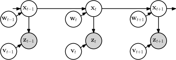
Figure 1: Graphical model of the dynamic system. The shaded nodes are the measured variables ${\boldsymbol{\mathbf{z}}}_{t}$, the unshaded nodes are unobserved variables. The arrows represent probabilistic dependencies between the variables.

The noise covariance matrices ${\mathbf{Q}}$, ${\mathbf{R}}$, the system function $f$, and the measurement function $g$ are assumed known. If not stated otherwise, we assume nonlinear functions $f$ and $g$. The initial state ${\boldsymbol{\mathbf{x}}}_{0}$ of the time series is distributed according to a Gaussian prior distribution ${p}({\boldsymbol{\mathbf{x}}}_{0})=\mathcal{N}({\boldsymbol{\mathbf{\mu}}}_{0}^{x},{\mathbf{\Sigma}}_{0}^{x})$. The purpose of filtering and smoothing is to find approximations to the posterior distributions ${p}({\boldsymbol{\mathbf{x}}}_{t}|{\boldsymbol{\mathbf{z}}}_{1:\tau})$, where a subscript $1\!:\!\tau$ abbreviates $1,\dotsc,\tau$, with $\tau\!=\!t$ for filtering and $\tau\!=\!T$ for smoothing.

In this paper, we consider Gaussian approximations $\mathcal{N}({\boldsymbol{\mathbf{x}}}_{t}\,|\,{\boldsymbol{\mathbf{\mu}}}_{t|\tau}^{x},{\mathbf{\Sigma}}_{t|\tau}^{x})$ of the latent state posteriors ${p}({\boldsymbol{\mathbf{x}}}_{t}|{\boldsymbol{\mathbf{z}}}_{1:\tau})$. We use the shorthand notation ${\boldsymbol{\mathbf{a}}}_{b|c}^{d}$ where ${\boldsymbol{\mathbf{a}}}={\boldsymbol{\mathbf{\mu}}}$ denotes the mean ${\boldsymbol{\mathbf{\mu}}}$ and ${\boldsymbol{\mathbf{a}}}={\mathbf{\Sigma}}$ denotes the covariance, $b$ denotes the time step under consideration, $c$ denotes the time step up to which we consider measurements, and $d\in\{x,z\}$ denotes either the latent space ($x$) or the observed space ($z$).

Let us assume a prior ${p}({\boldsymbol{\mathbf{x}}}_{0})={p}({\boldsymbol{\mathbf{x}}}_{0}|\emptyset)$ and a sequence ${{\boldsymbol{\mathbf{z}}}}_{1},\dotsc,{\boldsymbol{\mathbf{z}}}_{T}$ of noisy measurements of the latent states ${\boldsymbol{\mathbf{x}}}_{0},\dotsc,{\boldsymbol{\mathbf{x}}}_{T}$ through the measurement function $g$. The objective of filtering is to compute a posterior distribution ${p}({\boldsymbol{\mathbf{x}}}_{t}|{{\boldsymbol{\mathbf{z}}}}_{1:t})$ over the latent state as soon as a new measurement ${\boldsymbol{\mathbf{z}}}_{t}$ is available. Smoothing extends filtering and aims to compute the posterior state distribution of the hidden states ${\boldsymbol{\mathbf{x}}}_{t}$, $t=0,\dotsc,T$, given all measurements ${\boldsymbol{\mathbf{z}}}_{1},\dotsc,{\boldsymbol{\mathbf{z}}}_{T}$ (see e.g., [1, 22]).

2 Gaussian Filtering

Given a prior ${p}({\boldsymbol{\mathbf{x}}}_{0})$ on the initial state and a dynamic system (e.g., Eqs. (1)–(2)), the objective of filtering is to infer a posterior distribution ${p}({\boldsymbol{\mathbf{x}}}_{t}|{\boldsymbol{\mathbf{z}}}_{1:t})$ of the hidden state ${\boldsymbol{\mathbf{x}}}_{t}$, $t=1,\dotsc,T$, incorporating the evidence of the measurements ${\boldsymbol{\mathbf{z}}}_{1:t}$. Specific for Gaussian filtering is that posterior distributions are approximated by Gaussians [22]. Approximations are required since generally a Gaussian distribution mapped through a nonlinear function does not stay Gaussian.

Assume a Gaussian filter distribution ${p}({\boldsymbol{\mathbf{x}}}_{t-1}|{{\boldsymbol{\mathbf{z}}}}_{1:t-1})=\mathcal{N}({\boldsymbol{\mathbf{\mu}}}_{t-1|t-1}^{x},{\mathbf{\Sigma}}_{t-1|t-1}^{x})$ is given (if not, we employ the prior ${p}({\boldsymbol{\mathbf{x}}}_{0})={p}({\boldsymbol{\mathbf{x}}}_{0}|\emptyset)=\mathcal{N}({\boldsymbol{\mathbf{\mu}}}_{0|\emptyset}^{x},{\mathbf{\Sigma}}_{0|\emptyset}^{x}))$ on the initial state. Using Bayes’ theorem, the filter distribution at time $t$ is

$${p}({\boldsymbol{\mathbf{x}}}_{t}|{{\boldsymbol{\mathbf{z}}}}_{1:t}) =\frac{{p}({\boldsymbol{\mathbf{x}}}_{t},{\boldsymbol{\mathbf{z}}}_{t}|{\boldsymbol{\mathbf{z}}}_{1:t-1})}{{p}({\boldsymbol{\mathbf{z}}}_{t}|{\boldsymbol{\mathbf{z}}}_{1:t-1})}\propto{p}({\boldsymbol{\mathbf{z}}}_{t}|{\boldsymbol{\mathbf{x}}}_{t}){p}({\boldsymbol{\mathbf{x}}}_{t}|{\boldsymbol{\mathbf{z}}}_{1:t-1})\,.$$ (3)

Proposition 1 (Filter Distribution).

Gaussian filters approximate the filter distribution ${p}({\boldsymbol{\mathbf{x}}}_{t}|{\boldsymbol{\mathbf{z}}}_{1:t})$ using a Gaussian distribution $\mathcal{N}({\boldsymbol{\mathbf{\mu}}}_{t|t}^{x},{\mathbf{\Sigma}}_{t|t}^{x})$. The moments of this approximation are in general computed through

$${\boldsymbol{\mathbf{\mu}}}_{t|t}^{x} =\hat{{\boldsymbol{\mathbf{\mu}}}}_{t|t-1}^{x}+\hat{{\mathbf{\Sigma}}}_{t|t-1}^{xz}(\hat{{\mathbf{\Sigma}}}_{t|t-1}^{z})^{-1}({\boldsymbol{\mathbf{z}}}_{t}-\hat{{\boldsymbol{\mathbf{\mu}}}}_{t|t-1}^{z})\,,$$ (4)

$${\mathbf{\Sigma}}_{t|t}^{x} =\hat{{\mathbf{\Sigma}}}_{t|t-1}^{x}-\hat{{\mathbf{\Sigma}}}_{t|t-1}^{xz}(\hat{{\mathbf{\Sigma}}}_{t|t-1}^{z})^{-1}\hat{{\mathbf{\Sigma}}}_{t|t-1}^{zx}\,.$$ (5)

Since the true moments of the joint distribution ${p}({\boldsymbol{\mathbf{x}}}_{t},{\boldsymbol{\mathbf{z}}}_{t}|{\boldsymbol{\mathbf{z}}}_{1:t-1})$ can in general not be computed analytically, approximations/estimates are used (hence the $\hat{~{}}$-symbols).

Proof.

Generally, filtering proceeds by alternating between predicting (time update) and correcting (measurement update) [1, 22]:

1. Time update (predictor)

   1. Compute the predictive distribution ${p}({\boldsymbol{\mathbf{x}}}_{t}|{\boldsymbol{\mathbf{z}}}_{1:t-1})$.

2. Measurement update (corrector)

   1. Compute the joint distribution ${p}({\boldsymbol{\mathbf{x}}}_{t},{\boldsymbol{\mathbf{z}}}_{t}|{{\boldsymbol{\mathbf{z}}}}_{1:t-1})$ of the next latent state and the next measurement.

   2. Measure ${\boldsymbol{\mathbf{z}}}_{t}$.

   3. Compute the posterior ${p}({\boldsymbol{\mathbf{x}}}_{t}|{{\boldsymbol{\mathbf{z}}}}_{1:t})$.

In the following, we detail these steps to prove Prop. 1.

2.1 Time Update (Predictor)

1. Compute the predictive distribution ${p}({\boldsymbol{\mathbf{x}}}_{t}|{\boldsymbol{\mathbf{z}}}_{1:t-1})$. The predictive distribution of state ${\boldsymbol{\mathbf{x}}}$ at time $t$ given the evidence of measurements up to time $t-1$ is

   $${p}({\boldsymbol{\mathbf{x}}}_{t}|{\boldsymbol{\mathbf{z}}}_{1:t-1})\!=\!\int\!{p}({\boldsymbol{\mathbf{x}}}_{t}|{\boldsymbol{\mathbf{x}}}_{t-1}){p}({\boldsymbol{\mathbf{x}}}_{t-1}|{\boldsymbol{\mathbf{z}}}_{1:t-1})\operatorname{d}\!{\boldsymbol{\mathbf{x}}}_{t-1}\,,$$ (6)

   where ${p}({\boldsymbol{\mathbf{x}}}_{t}|{\boldsymbol{\mathbf{x}}}_{t-1})=\mathcal{N}({\boldsymbol{\mathbf{x}}}_{t}\,|\,f({\boldsymbol{\mathbf{x}}}_{t-1}),{\mathbf{Q}})$ is the transition probability. In Gaussian filters, the predictive distribution ${p}({\boldsymbol{\mathbf{x}}}_{t}|{\boldsymbol{\mathbf{z}}}_{1:t-1})$ in Eq. (6) is approximated by a Gaussian distribution, whose exact mean and covariance are given by

   $${\boldsymbol{\mathbf{\mu}}}_{t|t-1}^{x} \!\coloneqq\!\mathds{E}_{{\boldsymbol{\mathbf{x}}}_{t}}[{\boldsymbol{\mathbf{x}}}_{t}|{\boldsymbol{\mathbf{z}}}_{1:t-1}]\!=\!\mathds{E}_{{\boldsymbol{\mathbf{x}}}_{t-1},{\boldsymbol{\mathbf{w}}}_{t}}[f({\boldsymbol{\mathbf{x}}}_{t-1})\!+\!{\boldsymbol{\mathbf{w}}}_{t}|{\boldsymbol{\mathbf{z}}}_{1:t-1}]=\int f({\boldsymbol{\mathbf{x}}}_{t-1}){p}({\boldsymbol{\mathbf{x}}}_{t-1}|{\boldsymbol{\mathbf{z}}}_{1:t-1})\operatorname{d}\!{\boldsymbol{\mathbf{x}}}_{t-1}\,,$$ (7)

   $${\mathbf{\Sigma}}_{t|t-1}^{x} \coloneqq\mathrm{cov}_{{\boldsymbol{\mathbf{x}}}_{t}}[{\boldsymbol{\mathbf{x}}}_{t}|{\boldsymbol{\mathbf{z}}}_{1:t-1}]=\mathrm{cov}_{{\boldsymbol{\mathbf{x}}}_{t-1}}[f({\boldsymbol{\mathbf{x}}}_{t-1})|{\boldsymbol{\mathbf{z}}}_{1:t-1}]+\mathrm{cov}_{{\boldsymbol{\mathbf{w}}}_{t}}[{\boldsymbol{\mathbf{w}}}_{t}]$$

   $$=\underbrace{\int f({\boldsymbol{\mathbf{x}}}_{t-1})f({\boldsymbol{\mathbf{x}}}_{t-1})^{\top}{p}({\boldsymbol{\mathbf{x}}}_{t-1}|{\boldsymbol{\mathbf{z}}}_{1:t-1})\operatorname{d}\!{\boldsymbol{\mathbf{x}}}_{t-1}-{\boldsymbol{\mathbf{\mu}}}_{t|t-1}^{x}\big{(}{\boldsymbol{\mathbf{\mu}}}_{t|t-1}^{x})^{\top}}_{=\mathrm{cov}_{{\boldsymbol{\mathbf{x}}}_{t-1}}[f({\boldsymbol{\mathbf{x}}}_{t-1})|{\boldsymbol{\mathbf{z}}}_{1:t-1}]}+\underbrace{{\mathbf{Q}}}_{=\mathrm{cov}_{{\boldsymbol{\mathbf{w}}}_{t}}[{\boldsymbol{\mathbf{w}}}_{t}]}$$ (8)

   respectively. In Eq. (7), we exploited that the noise term ${\boldsymbol{\mathbf{w}}}_{t}$ in Eq. (1) has mean zero and is independent. A Gaussian approximation to the time update ${p}({\boldsymbol{\mathbf{x}}}_{t}|{\boldsymbol{\mathbf{z}}}_{1:t-1})$ is then given by $\mathcal{N}({\boldsymbol{\mathbf{x}}}_{t}\,|\,{\boldsymbol{\mathbf{\mu}}}_{t|t-1}^{x},{\mathbf{\Sigma}}_{t|t-1}^{x})$.

2.2 Measurement Update (Corrector)

1. Compute the joint distribution

   $${p}({\boldsymbol{\mathbf{x}}}_{t},{\boldsymbol{\mathbf{z}}}_{t}|{\boldsymbol{\mathbf{z}}}_{1:t-1})={p}({\boldsymbol{\mathbf{z}}}_{t}|{\boldsymbol{\mathbf{x}}}_{t})\underbrace{{p}({\boldsymbol{\mathbf{x}}}_{t}|{\boldsymbol{\mathbf{z}}}_{1:t-1})}_{\text{time update}}\,.$$ (9)

   In Gaussian filters, a Gaussian approximation to this joint is an intermediate step toward the desired Gaussian approximation of the posterior ${p}({\boldsymbol{\mathbf{x}}}_{t}|{\boldsymbol{\mathbf{z}}}_{1:t})$. If the mean and the covariance of the joint in Eq. (9) can be computed or estimated, the desired filter distribution corresponds to the conditional ${p}({\boldsymbol{\mathbf{x}}}_{t}|{\boldsymbol{\mathbf{z}}}_{1:t})$ and is given in closed form [3].

   Our objective is to compute a Gaussian approximation

   $$\mathcal{N}\left(\begin{bmatrix}{\boldsymbol{\mathbf{\mu}}}_{t|t-1}^{x}\\ {\boldsymbol{\mathbf{\mu}}}_{t|t-1}^{z}\end{bmatrix},\begin{bmatrix}{\mathbf{\Sigma}}_{t|t-1}^{x}&{\mathbf{\Sigma}}_{t|t-1}^{xz}\\ {\mathbf{\Sigma}}_{t|t-1}^{zx}&{\mathbf{\Sigma}}_{t|t-1}^{z}\end{bmatrix}\right)$$ (10)

   to the joint ${p}({\boldsymbol{\mathbf{x}}}_{t},{\boldsymbol{\mathbf{z}}}_{t}|{\boldsymbol{\mathbf{z}}}_{1:t-1})$ in Eq. (9). Since a Gaussian approximation $\mathcal{N}({\boldsymbol{\mathbf{\mu}}}_{t|t-1}^{x},{\mathbf{\Sigma}}_{t|t-1}^{x})$ to the marginal ${p}({\boldsymbol{\mathbf{x}}}_{t}|{\boldsymbol{\mathbf{z}}}_{1:t-1})$ is known from the time update, it remains to compute the marginal ${p}({\boldsymbol{\mathbf{z}}}_{t}|{\boldsymbol{\mathbf{z}}}_{1:t-1})$ and the cross-covariance ${\mathbf{\Sigma}}_{t|t-1}^{xz}\coloneqq\mathrm{cov}_{{\boldsymbol{\mathbf{x}}}_{t},{\boldsymbol{\mathbf{z}}}_{t}}[{\boldsymbol{\mathbf{x}}}_{t},{\boldsymbol{\mathbf{z}}}_{t}|{\boldsymbol{\mathbf{z}}}_{1:t-1}]$.

   • The marginal ${p}({\boldsymbol{\mathbf{z}}}_{t}|{{\boldsymbol{\mathbf{z}}}}_{1:t-1})$ of the joint in Eq. (10) is

     $${p}({\boldsymbol{\mathbf{z}}}_{t}|{\boldsymbol{\mathbf{z}}}_{1:t-1})=\int{p}({\boldsymbol{\mathbf{z}}}_{t}|{\boldsymbol{\mathbf{x}}}_{t}){p}({\boldsymbol{\mathbf{x}}}_{t}|{\boldsymbol{\mathbf{z}}}_{1:t-1})\operatorname{d}\!{\boldsymbol{\mathbf{x}}}_{t}\,,$$

     where the state ${\boldsymbol{\mathbf{x}}}_{t}$ is integrated out according to the time update ${p}({\boldsymbol{\mathbf{x}}}_{t}|{\boldsymbol{\mathbf{z}}}_{1:t-1})$. The measurement Eq. (2), yields ${p}({\boldsymbol{\mathbf{z}}}_{t}|{\boldsymbol{\mathbf{x}}}_{t})=\mathcal{N}(g({\boldsymbol{\mathbf{x}}}_{t}),{\mathbf{R}})$. Hence, the exact mean of the marginal is

     $${\boldsymbol{\mathbf{\mu}}}_{t|t-1}^{z} \coloneqq\mathds{E}_{{\boldsymbol{\mathbf{z}}}_{t}}[{\boldsymbol{\mathbf{z}}}_{t}|{\boldsymbol{\mathbf{z}}}_{1:t-1}]=\mathds{E}_{{\boldsymbol{\mathbf{x}}}_{t}}[g({\boldsymbol{\mathbf{x}}}_{t})|{\boldsymbol{\mathbf{z}}}_{1:t-1}]=\int g({\boldsymbol{\mathbf{x}}}_{t})\underbrace{{p}({\boldsymbol{\mathbf{x}}}_{t}|{\boldsymbol{\mathbf{z}}}_{1:t-1})}_{\text{time update}}\operatorname{d}\!{\boldsymbol{\mathbf{x}}}_{t}$$ (11)

     since the noise term ${\boldsymbol{\mathbf{v}}}_{t}$ in the measurement Eq. (2) is independent and has zero mean. Similarly, the exact covariance of the marginal ${p}({\boldsymbol{\mathbf{z}}}_{t}|{\boldsymbol{\mathbf{z}}}_{1:t-1})$ is

     $${\mathbf{\Sigma}}_{t|t-1}^{z} =\mathrm{cov}_{{\boldsymbol{\mathbf{z}}}_{t}}[{\boldsymbol{\mathbf{z}}}_{t}|{\boldsymbol{\mathbf{z}}}_{1:t-1}=\mathrm{cov}_{{\boldsymbol{\mathbf{x}}}_{t}}[g({\boldsymbol{\mathbf{x}}}_{t})|{\boldsymbol{\mathbf{z}}}_{1:t-1}]+\mathrm{cov}_{{\boldsymbol{\mathbf{v}}}_{t}}[{\boldsymbol{\mathbf{v}}}_{t}]$$

     $$=\underbrace{\int g({\boldsymbol{\mathbf{x}}}_{t})g({\boldsymbol{\mathbf{x}}}_{t})^{\top}{p}({\boldsymbol{\mathbf{x}}}_{t}|{\boldsymbol{\mathbf{z}}}_{1:t-1})\operatorname{d}\!{\boldsymbol{\mathbf{x}}}_{t}-{\boldsymbol{\mathbf{\mu}}}_{t|t-1}^{z}\big{(}{\boldsymbol{\mathbf{\mu}}}_{t|t-1}^{z})^{\top}}_{=\mathrm{cov}_{{\boldsymbol{\mathbf{x}}}_{t}}[g({\boldsymbol{\mathbf{x}}}_{t})|{\boldsymbol{\mathbf{z}}}_{1:t-1}]}+\underbrace{{\mathbf{R}}}_{=\mathrm{cov}_{{\boldsymbol{\mathbf{v}}}_{t}}[{\boldsymbol{\mathbf{v}}}_{t}]}\,.$$ (12)

     Hence, a Gaussian approximation to the marginal measurement distribution ${p}({\boldsymbol{\mathbf{z}}}_{t}|{\boldsymbol{\mathbf{z}}}_{1:t-1})$ is given by

     $$\mathcal{N}({\boldsymbol{\mathbf{z}}}_{t}\,|\,{\boldsymbol{\mathbf{\mu}}}_{t|t-1}^{z},{\mathbf{\Sigma}}_{t|t-1}^{z})\,,$$ (13)

     with the mean and covariance given in Eqs. (11) and (12), respectively.

   • Due to the independence of ${\boldsymbol{\mathbf{v}}}_{t}$, the exact cross-covariance terms of the joint in Eq. (10) are

     $${\mathbf{\Sigma}}_{t|t-1}^{xz} =\mathrm{cov}_{{\boldsymbol{\mathbf{x}}}_{t},{\boldsymbol{\mathbf{z}}}_{t}}[{\boldsymbol{\mathbf{x}}}_{t},{\boldsymbol{\mathbf{z}}}_{t}|{\boldsymbol{\mathbf{z}}}_{1:t-1}]=\mathds{E}_{{\boldsymbol{\mathbf{x}}}_{t},{\boldsymbol{\mathbf{z}}}_{t}}[{\boldsymbol{\mathbf{x}}}_{t}{\boldsymbol{\mathbf{z}}}_{t}^{\top}|{\boldsymbol{\mathbf{z}}}_{1:t-1}]-\mathds{E}_{{\boldsymbol{\mathbf{x}}}_{t}}[{\boldsymbol{\mathbf{x}}}_{t}|{\boldsymbol{\mathbf{z}}}_{1:t-1}]\mathds{E}_{{\boldsymbol{\mathbf{z}}}_{t}}[{\boldsymbol{\mathbf{z}}}_{t}|{\boldsymbol{\mathbf{z}}}_{1:t-1}]^{\top}$$

     $$=\iint{\boldsymbol{\mathbf{x}}}_{t}{\boldsymbol{\mathbf{z}}}_{t}^{\top}{p}({\boldsymbol{\mathbf{x}}}_{t},{\boldsymbol{\mathbf{z}}}_{t}|{\boldsymbol{\mathbf{z}}}_{1:t-1})\operatorname{d}\!{\boldsymbol{\mathbf{z}}}_{t}\operatorname{d}\!{\boldsymbol{\mathbf{x}}}_{t}-{\boldsymbol{\mathbf{\mu}}}_{t|t-1}^{x}({\boldsymbol{\mathbf{\mu}}}_{t|t-1}^{z})^{\top}\,.$$

     Plugging in the measurement Eq. (2), we obtain

     $${\mathbf{\Sigma}}_{t|t-1}^{xz} =\int{\boldsymbol{\mathbf{x}}}_{t}g({\boldsymbol{\mathbf{x}}}_{t})^{\top}{p}({\boldsymbol{\mathbf{x}}}_{t}|{\boldsymbol{\mathbf{z}}}_{1:t-1})\operatorname{d}\!{\boldsymbol{\mathbf{x}}}_{t}-{\boldsymbol{\mathbf{\mu}}}_{t|t-1}^{x}({\boldsymbol{\mathbf{\mu}}}_{t|t-1}^{z})^{\top}\,.$$ (14)

2. Measure ${\boldsymbol{\mathbf{z}}}_{t}$.

3. Compute a Gaussian approximation of the posterior ${p}({\boldsymbol{\mathbf{x}}}_{t}|{\boldsymbol{\mathbf{z}}}_{1:t})$. This boils down to computing a conditional from the Gaussian approximation to the joint distribution ${p}({\boldsymbol{\mathbf{x}}}_{t},{\boldsymbol{\mathbf{z}}}_{t}|{\boldsymbol{\mathbf{z}}}_{1:t-1})$ in Eq. (10). The expressions from Eqs. (7), (8), (11), (12), and (14), yield a Gaussian approximation $\mathcal{N}({\boldsymbol{\mathbf{x}}}_{t}\,|\,{\boldsymbol{\mathbf{\mu}}}_{t|t}^{x},{\mathbf{\Sigma}}_{t|t}^{x})$ of the filter distribution ${p}({\boldsymbol{\mathbf{x}}}_{t}|{\boldsymbol{\mathbf{z}}}_{1:t})$, where

   $${\boldsymbol{\mathbf{\mu}}}_{t|t}^{x} ={\boldsymbol{\mathbf{\mu}}}_{t|t-1}^{x}+{\mathbf{\Sigma}}_{t|t-1}^{xz}\big{(}{\mathbf{\Sigma}}_{t|t-1}^{z}\big{)}^{-1}({\boldsymbol{\mathbf{z}}}_{t}-{\boldsymbol{\mathbf{\mu}}}_{t|t-1}^{z})\,,$$ (15)

   $${\mathbf{\Sigma}}_{t|t}^{x} ={\mathbf{\Sigma}}_{t|t-1}^{x}-{\mathbf{\Sigma}}_{t|t-1}^{xz}\big{(}{\mathbf{\Sigma}}_{t|t-1}^{z}\big{)}^{-1}{\mathbf{\Sigma}}_{t|t-1}^{zx}\,.$$ (16)

Generally, the required integrals in Eqs. (7), (8), (11), (12), and (14) cannot be computed analytically. Hence, approximations of the moments are typically used in Eqs. (15) and (16). This concludes the proof of Prop. 1. ∎

2.3 Sufficient Conditions for Gaussian Filtering

In any Bayes filter [22], the sufficient components to computing the Gaussian filter distribution in Eqs. (15) and (16) are the mean and the covariance of the joint distribution ${p}({\boldsymbol{\mathbf{x}}}_{t},{\boldsymbol{\mathbf{z}}}_{t}|{\boldsymbol{\mathbf{z}}}_{1:t-1})$. Generally, the required integrals in Eqs. (7), (8), (11), (12), and (14) cannot be computed analytically. One exception are linear functions $f$ and $g$, where the analytic solutions to the integrals are embodied in the Kalman filter [12]: Using the rules of predicting in linear Gaussian systems, the Kalman filter equations can be recovered when plugging in the respective means and covariances into Eq. (15) and (16) [20, 16, 1, 3, 22]. In many nonlinear dynamic systems, filtering algorithms approximate probability distributions (see e.g., the UKF [11] and the CKF [2]) or the functions $f$ and $g$ (see e.g., the EKF [15] or the GP-Bayes filters [6, 13]). Using the means and (cross-)covariances computed by these algorithms and plugging them into Eqs. (15)–(16), recovers the corresponding filter update equations for the EKF, the UKF, the CKF, and the GP-Bayes filters.

3 Gaussian RTS Smoothing

In this section, we present a general probabilistic perspective on Gaussian RTS smoothers and derive sufficient conditions for Gaussian smoothing.

The smoothed state distribution is the posterior distribution of the hidden state given all measurements

$${p}({\boldsymbol{\mathbf{x}}}_{t}|{\boldsymbol{\mathbf{z}}}_{1:T})\,,\,\,t=T,\dotsc,0\,.$$ (17)

Proposition 2 (Smoothing Distribution).

For Gaussian smoothers, the mean and the covariance of a Gaussian approximation to the distribution ${p}({\boldsymbol{\mathbf{x}}}_{t}|{\boldsymbol{\mathbf{z}}}_{1:T})$ are generally computed as

$${\boldsymbol{\mathbf{\mu}}}_{t-1|T}^{x} =\hat{{\boldsymbol{\mathbf{\mu}}}}_{t-1|t-1}^{x}+\hat{{\mathbf{J}}}_{t-1}(\hat{{\boldsymbol{\mathbf{\mu}}}}_{t|T}^{x}-\hat{{\boldsymbol{\mathbf{\mu}}}}_{t|t-1}^{x})\,,$$ (18)

$${\mathbf{\Sigma}}_{t-1|T}^{x} =\hat{{\mathbf{\Sigma}}}_{t-1|t-1}^{x}+\hat{{\mathbf{J}}}_{t-1}(\hat{{\mathbf{\Sigma}}}_{t|T}^{x}-\hat{{\mathbf{\Sigma}}}_{t|t-1}^{x})\hat{{\mathbf{J}}}_{t-1}^{\top}\,,$$ (19)

$${\mathbf{J}}_{t-1} =\mathrm{cov}[{\boldsymbol{\mathbf{x}}}_{t-1},{\boldsymbol{\mathbf{x}}}_{t}|{\boldsymbol{\mathbf{z}}}_{1:t-1}]\mathrm{cov}[{\boldsymbol{\mathbf{x}}}_{t}|{\boldsymbol{\mathbf{z}}}_{1:t-1}]^{-1}$$

$$={\mathbf{\Sigma}}_{t-1,t|t-1}^{x}({\mathbf{\Sigma}}_{t|t-1}^{x})^{-1}\,.$$ (20)

Proof.

The smoothed state distribution at the terminal time step $T$ is equivalent to the filter distribution ${p}({\boldsymbol{\mathbf{x}}}_{T}|{\boldsymbol{\mathbf{z}}}_{1:T})$ [1, 3]. The distributions ${p}({\boldsymbol{\mathbf{x}}}_{t-1}|{\boldsymbol{\mathbf{z}}}_{1:T})$, $t=T,\dotsc,1$, of the smoothed states can be computed recursively according to

$${p}({\boldsymbol{\mathbf{x}}}_{t-1}|{\boldsymbol{\mathbf{z}}}_{1:T}) =\int{p}({\boldsymbol{\mathbf{x}}}_{t-1}|{\boldsymbol{\mathbf{x}}}_{t},{\boldsymbol{\mathbf{z}}}_{1:T}){p}({\boldsymbol{\mathbf{x}}}_{t}|{\boldsymbol{\mathbf{z}}}_{1:T})\operatorname{d}\!{\boldsymbol{\mathbf{x}}}_{t}=\int{p}({\boldsymbol{\mathbf{x}}}_{t-1}|{\boldsymbol{\mathbf{x}}}_{t},{\boldsymbol{\mathbf{z}}}_{1:t-1}){p}({\boldsymbol{\mathbf{x}}}_{t}|{\boldsymbol{\mathbf{z}}}_{1:T})\operatorname{d}\!{\boldsymbol{\mathbf{x}}}_{t}$$ (21)

by integrating out the smoothed hidden state at time step $t$. In Eq. (21), we exploited that ${\boldsymbol{\mathbf{x}}}_{t-1}$ is conditionally independent of the future measurements ${\boldsymbol{\mathbf{z}}}_{t:T}$ given ${\boldsymbol{\mathbf{x}}}_{t}$.

To compute the smoothed state distribution in Eq. (21), we need to multiply a distribution in ${\boldsymbol{\mathbf{x}}}_{t}$ with a distribution in ${\boldsymbol{\mathbf{x}}}_{t-1}$ and integrate over ${\boldsymbol{\mathbf{x}}}_{t}$. To do so, we follow the steps:

1. Compute the conditional ${p}({\boldsymbol{\mathbf{x}}}_{t-1}|{\boldsymbol{\mathbf{x}}}_{t},{\boldsymbol{\mathbf{z}}}_{1:t-1})$.

2. Formulate ${p}({\boldsymbol{\mathbf{x}}}_{t-1}|{\boldsymbol{\mathbf{x}}}_{t},{\boldsymbol{\mathbf{z}}}_{1:T})$ as an unnormalized distribution in ${\boldsymbol{\mathbf{x}}}_{t}$.

3. Multiply the new distribution with ${p}({\boldsymbol{\mathbf{x}}}_{t}|{\boldsymbol{\mathbf{z}}}_{1:T})$.

4. Solve the integral in Eq. (21).

We now examine these steps in detail. Assume a known (Gaussian) smoothed state distribution ${p}({\boldsymbol{\mathbf{x}}}_{t}|{\boldsymbol{\mathbf{z}}}_{1:T})$.

1. Compute a Gaussian approximation to the conditional ${p}({\boldsymbol{\mathbf{x}}}_{t-1}|{\boldsymbol{\mathbf{x}}}_{t},{\boldsymbol{\mathbf{z}}}_{1:t-1})$. We compute the conditional in two steps: First, we compute a Gaussian approximation to the joint distribution ${p}({\boldsymbol{\mathbf{x}}}_{t},{\boldsymbol{\mathbf{x}}}_{t-1}|{\boldsymbol{\mathbf{z}}}_{1:t-1})$. Second, we apply the rules of computing conditionals to this joint Gaussian. Let us start with a Gaussian approximation

   $$\mathcal{N}\left(\begin{bmatrix}{\boldsymbol{\mathbf{\mu}}}_{t-1|t-1}^{x}\\ {\boldsymbol{\mathbf{\mu}}}_{t|t-1}^{x}\end{bmatrix},\begin{bmatrix}{\mathbf{\Sigma}}_{t-1|t-1}^{x}&{\mathbf{\Sigma}}_{t-1,t|t-1}^{x}\\ ({\mathbf{\Sigma}}_{t-1,t|t-1}^{x})^{\top}&{\mathbf{\Sigma}}_{t|t-1}^{x}\end{bmatrix}\right)$$ (22)

   to the joint ${p}({\boldsymbol{\mathbf{x}}}_{t-1},{\boldsymbol{\mathbf{x}}}_{t}|{\boldsymbol{\mathbf{z}}}_{1:t-1})$ and have a closer look at its components: A Gaussian approximation of the filter distribution ${p}({\boldsymbol{\mathbf{x}}}_{t-1}|{\boldsymbol{\mathbf{z}}}_{1:t-1})$ at time step $t-1$ is known and is the first marginal distribution in Eq. (22). The second marginal $\mathcal{N}({\boldsymbol{\mathbf{\mu}}}_{t|t-1}^{x},{\mathbf{\Sigma}}_{t|t-1}^{x})$ is the time update and also known from filtering. To fully determine the joint in Eq. (22), we require the cross-covariance matrix

   $${\mathbf{\Sigma}}_{t-1,t|t-1}^{x} =\iint{\boldsymbol{\mathbf{x}}}_{t-1}f({\boldsymbol{\mathbf{x}}}_{t-1})^{\top}{p}({\boldsymbol{\mathbf{x}}}_{t-1}|{\boldsymbol{\mathbf{z}}}_{1:t-1})\operatorname{d}\!{\boldsymbol{\mathbf{x}}}_{t-1}-{\boldsymbol{\mathbf{\mu}}}_{t-1|t-1}^{x}({\boldsymbol{\mathbf{\mu}}}_{t|t-1}^{x})^{\top}\,,$$ (23)

   where we used the means ${\boldsymbol{\mathbf{\mu}}}_{t-1|t-1}^{x}$ and ${\boldsymbol{\mathbf{\mu}}}_{t|t-1}^{x}$ of the measurement update and the time update, respectively. The zero-mean independent noise in the system Eq. (1) does not influence the cross-covariance matrix. The cross-covariance matrix in Eq. (23) can be pre-computed during filtering since it does not depend on future measurements.

   This concludes the first step (computation of the joint Gaussian) of the computation of the desired conditional.

   In the second step, we apply the rules of Gaussian conditioning to obtain the desired conditional distribution ${p}({\boldsymbol{\mathbf{x}}}_{t-1}|{\boldsymbol{\mathbf{x}}}_{t},{\boldsymbol{\mathbf{z}}}_{1:t-1})$. For a shorthand notation, we define

   $${\mathbf{J}}_{t-1}\coloneqq{\mathbf{\Sigma}}_{t-1,t|t-1}^{x}({\mathbf{\Sigma}}_{t|t-1}^{x})^{-1}\,,$$ (24)

   and obtain a Gaussian approximation $\mathcal{N}({\boldsymbol{\mathbf{x}}}_{t-1}\,|\,{\boldsymbol{\mathbf{m}}},{\mathbf{S}})$ of the conditional distribution ${p}({\boldsymbol{\mathbf{x}}}_{t-1}|{\boldsymbol{\mathbf{x}}}_{t},{\boldsymbol{\mathbf{z}}}_{1:t-1})$ with

   $${\boldsymbol{\mathbf{m}}} ={\boldsymbol{\mathbf{\mu}}}_{t-1|t-1}^{x}+{\mathbf{J}}_{t-1}({\boldsymbol{\mathbf{x}}}_{t}-{\boldsymbol{\mathbf{\mu}}}_{t|t-1}^{x})\,,$$ (25)

   $${\mathbf{S}} ={\mathbf{\Sigma}}_{t-1|t-1}^{x}-{\mathbf{J}}_{t-1}({\mathbf{\Sigma}}_{t-1,t|t-1}^{x})^{\top}\,.$$ (26)

2. Formulate $\mathcal{N}({\boldsymbol{\mathbf{x}}}_{t-1}\,|\,{\boldsymbol{\mathbf{m}}},{\mathbf{S}})$ as an unnormalized distribution in ${\boldsymbol{\mathbf{x}}}_{t}$. The square-root of the exponent of $\mathcal{N}({\boldsymbol{\mathbf{x}}}_{t-1}\,|\,{\boldsymbol{\mathbf{m}}},{\mathbf{S}})$ contains

   $${\boldsymbol{\mathbf{x}}}_{t-1}-{\boldsymbol{\mathbf{m}}} ={\boldsymbol{\mathbf{r}}}({\boldsymbol{\mathbf{x}}}_{t-1})-{\mathbf{J}}_{t-1}{\boldsymbol{\mathbf{x}}}_{t}$$

   with ${\boldsymbol{\mathbf{r}}}({\boldsymbol{\mathbf{x}}}_{t-1})={\boldsymbol{\mathbf{x}}}_{t-1}-{\boldsymbol{\mathbf{\mu}}}_{t-1|t-1}^{x}+{\mathbf{J}}_{t-1}{\boldsymbol{\mathbf{\mu}}}_{t|t-1}^{x}$, which is a linear function of both ${\boldsymbol{\mathbf{x}}}_{t-1}$ and ${\boldsymbol{\mathbf{x}}}_{t}$. We now reformulate the conditional Gaussian $\mathcal{N}({\boldsymbol{\mathbf{x}}}_{t-1}\,|\,{\boldsymbol{\mathbf{m}}},{\mathbf{S}})$ as a Gaussian in ${\mathbf{J}}_{t-1}{\boldsymbol{\mathbf{x}}}_{t}$ with mean ${\boldsymbol{\mathbf{r}}}({\boldsymbol{\mathbf{x}}}_{t-1})$ and the unchanged covariance matrix ${\mathbf{S}}$. We obtain the conditional

   $$\mathcal{N}({\boldsymbol{\mathbf{x}}}_{t-1}\,|\,{\boldsymbol{\mathbf{m}}},{\mathbf{S}}) =c_{1}\mathcal{N}({\boldsymbol{\mathbf{x}}}_{t}\,|\,{\boldsymbol{\mathbf{a}}},{\mathbf{A}})\,,$$ (27)

   $$\text{with}\quad c_{1} =\sqrt{|2\pi({\mathbf{J}}_{t-1}^{\top}{\mathbf{S}}^{-1}{\mathbf{J}}_{t-1})^{-1}|/|2\pi{\mathbf{S}}|}\,,$$

   and ${\boldsymbol{\mathbf{a}}}={\mathbf{J}}_{t-1}^{-1}{\boldsymbol{\mathbf{r}}}({\boldsymbol{\mathbf{x}}}_{t-1})\,,{\mathbf{A}}=({\mathbf{J}}_{t-1}^{\top}{\mathbf{S}}^{-1}{\mathbf{J}}_{t-1})^{-1}$. Note that $\mathcal{N}({\boldsymbol{\mathbf{x}}}_{t-1}\,|\,{\boldsymbol{\mathbf{m}}},{\mathbf{S}})$ is an unnormalized Gaussian in ${\boldsymbol{\mathbf{x}}}_{t}$, see Eq. (27). The matrix ${\mathbf{J}}_{t-1}$ defined in Eq. (24) is quadratic, but not necessarily invertible, in which case we take the pseudo-inverse. However, we will see that this inversion will be unnecessary to obtain the final result.

3. Multiply the new distribution with ${p}({\boldsymbol{\mathbf{x}}}_{t}|{\boldsymbol{\mathbf{z}}}_{1:T})$. To determine ${p}({\boldsymbol{\mathbf{x}}}_{t-1}|{\boldsymbol{\mathbf{z}}}_{1:T})$, we multiply the Gaussian in Eq. (27) with the smoothed Gaussian state distribution $\mathcal{N}({\boldsymbol{\mathbf{x}}}_{t}\,|\,{\boldsymbol{\mathbf{\mu}}}_{t|T}^{x},{\mathbf{\Sigma}}_{t|T}^{x})$, which yields the Gaussian approximation

   $$c_{1}\mathcal{N}({\boldsymbol{\mathbf{x}}}_{t}\,|\,{\boldsymbol{\mathbf{a}}},{\mathbf{A}})\mathcal{N}({\boldsymbol{\mathbf{x}}}_{t}\,|\,{\boldsymbol{\mathbf{\mu}}}_{t|T}^{x},{\mathbf{\Sigma}}_{t|T}^{x}) =c_{1}c_{2}({\boldsymbol{\mathbf{a}}})\mathcal{N}({\boldsymbol{\mathbf{x}}}_{t}\,|\,{\boldsymbol{\mathbf{b}}},{\mathbf{B}})$$ (28)

   of ${p}({\boldsymbol{\mathbf{x}}}_{t-1},{\boldsymbol{\mathbf{x}}}_{t}|{\boldsymbol{\mathbf{z}}}_{1:T})$, for some ${\boldsymbol{\mathbf{b}}}$, ${\mathbf{B}}$, where $c_{2}({\boldsymbol{\mathbf{a}}})$ is the inverse normalization constant of $\mathcal{N}({\boldsymbol{\mathbf{x}}}_{t}\,|\,{\boldsymbol{\mathbf{b}}},{\mathbf{B}})$.

4. Solve the integral in Eq. (21). Since we integrate over ${\boldsymbol{\mathbf{x}}}_{t}$ in Eq. (21), we are solely interested in the parts that make Eq. (28) unnormalized, i.e., the constants $c_{1}$ and $c_{2}({\boldsymbol{\mathbf{a}}})$, which are independent of ${\boldsymbol{\mathbf{x}}}_{t}$. The constant $c_{2}({\boldsymbol{\mathbf{a}}})$ in Eq. (28) can be rewritten as $c_{2}({\boldsymbol{\mathbf{x}}}_{t-1})$ by reversing the step that inverted the matrix ${\mathbf{J}}_{t-1}$, see Eq. (27). Then, $c_{2}({\boldsymbol{\mathbf{x}}}_{t-1})$ is given by

   $$c_{2}({\boldsymbol{\mathbf{x}}}_{t-1})=c_{1}^{-1}\mathcal{N}({\boldsymbol{\mathbf{x}}}_{t-1}\,|\,{\boldsymbol{\mathbf{\mu}}}_{t-1|T}^{x},{\mathbf{\Sigma}}_{t-1|T}^{x})\,,$$ (29)

   $${\boldsymbol{\mathbf{\mu}}}_{t-1|T}^{x}={\boldsymbol{\mathbf{\mu}}}_{t-1|t-1}^{x}+{\mathbf{J}}_{t-1}({\boldsymbol{\mathbf{\mu}}}_{t|T}^{x}-{\boldsymbol{\mathbf{\mu}}}_{t|t-1}^{x})\,,$$ (30)

   $${\mathbf{\Sigma}}_{t-1|T}^{x}={\mathbf{\Sigma}}_{t-1|t-1}^{x}+{\mathbf{J}}_{t-1}({\mathbf{\Sigma}}_{t|T}^{x}-{\mathbf{\Sigma}}_{t|t-1}^{x}){\mathbf{J}}_{t-1}^{\top}\,.$$ (31)

   Since $c_{1}c_{1}^{-1}=1$ (plug Eq. (29) into Eq. (28)), the desired smoothed state distribution is

   $${p}({\boldsymbol{\mathbf{x}}}_{t-1}|{\boldsymbol{\mathbf{z}}}_{1:T})=\mathcal{N}({\boldsymbol{\mathbf{x}}}_{t-1}\,|\,{\boldsymbol{\mathbf{\mu}}}_{t-1|T}^{x},{\mathbf{\Sigma}}_{t-1|T}^{x})\,,$$ (32)

   where the mean and the covariance are given in Eq. (30) and Eq. (31), respectively.

This result concludes the proof of Prop. 2. ∎

3.1 Sufficient Conditions for Smoothing

After filtering, to determine a Gaussian approximation to the distribution ${p}({\boldsymbol{\mathbf{x}}}_{t-1}|{\boldsymbol{\mathbf{z}}}_{1:T})$ of the smoothed state at time $t-1$, only a few additional ingredients are required: the matrix ${\mathbf{J}}_{t-1}$ in Eq. (24) and Gaussian approximations to the smoothed state distribution ${p}({\boldsymbol{\mathbf{x}}}_{t}|{\boldsymbol{\mathbf{z}}}_{1:T})$ at time $t$ and the predictive distribution ${p}({\boldsymbol{\mathbf{x}}}_{t}|{\boldsymbol{\mathbf{z}}}_{1:t-1})$. Everything but the matrix ${\mathbf{J}}_{t-1}$ can be precomputed either during filtering or in a previous step of the smoothing recursion. Note that ${\mathbf{J}}_{t-1}$ can also be precomputed during filtering.

Hence, for Gaussian RTS smoothing it is sufficient to determine Gaussian approximations to both the joint distribution ${p}({\boldsymbol{\mathbf{x}}}_{t},{\boldsymbol{\mathbf{z}}}_{t}|{\boldsymbol{\mathbf{z}}}_{1:t-1})$ of the state and the measurement for the filter step and the joint distribution ${p}({\boldsymbol{\mathbf{x}}}_{t-1},{\boldsymbol{\mathbf{x}}}_{t}|{\boldsymbol{\mathbf{z}}}_{1:t-1})$ of two consecutive states.

4 Implications and Theoretical Results

Using the results from Secs. 2 and 3, we conclude that for filtering and RTS smoothing it is sufficient to compute or estimate the means and the covariances of the joint distribution ${p}({\boldsymbol{\mathbf{x}}}_{t-1},{\boldsymbol{\mathbf{x}}}_{t}|{\boldsymbol{\mathbf{z}}}_{1:t-1})$ between two consecutive states (smoothing) and the joint distribution ${p}({\boldsymbol{\mathbf{x}}}_{t},{\boldsymbol{\mathbf{z}}}_{t}|{\boldsymbol{\mathbf{z}}}_{1:t-1})$ between a state and the subsequent measurement (filtering and smoothing). This result has two implications:

1. Gaussian filters/smoothers can be distinguished by their approximations to these joint distributions.

2. If there exists an algorithm to compute or to estimate the means and the covariances of the joint distributions ${p}({\boldsymbol{\mathbf{x}}},h({\boldsymbol{\mathbf{x}}}))$, where $h\in\{f,g\}$, the algorithm can be used for filtering and RTS smoothing.

In the following, we first consider common filtering and smoothing algorithms and describe how they compute Gaussian approximations to the joint distributions ${p}({\boldsymbol{\mathbf{x}}}_{t-1},{\boldsymbol{\mathbf{x}}}_{t}|{\boldsymbol{\mathbf{z}}}_{1:t-1})$ and ${p}({\boldsymbol{\mathbf{x}}}_{t},{\boldsymbol{\mathbf{z}}}_{t}|{\boldsymbol{\mathbf{z}}}_{1:t-1})$, respectively, which emphasizes the first implication (Sec. 4.1). After that, for the second implication of our results, we take an algorithm for estimating means and covariances of joint distributions and turn this algorithm into a filter/smoother (Sec. 4.2).

4.1 Current Algorithms for Computing the Joint Distributions

Table 1: Computing the means and the covariances of $p({\boldsymbol{\mathbf{x}}}_{t},{\boldsymbol{\mathbf{z}}}_{t}|{\boldsymbol{\mathbf{z}}}_{1:t-1})$ and $p({\boldsymbol{\mathbf{x}}}_{t-1},{\boldsymbol{\mathbf{x}}}_{t}|{\boldsymbol{\mathbf{z}}}_{1:t-1})$.

	Kalman filter/smoother	EKF/EKS	UKF/URTSS and CKF/CKS⋆
$\hat{{\boldsymbol{\mathbf{\mu}}}}_{t|t-1}^{x}$	${\boldsymbol{\mathbf{F}}}{\boldsymbol{\mathbf{\mu}}}_{t-1|t-1}^{x}$	$\tilde{{\boldsymbol{\mathbf{F}}}}\hat{{\boldsymbol{\mathbf{\mu}}}}_{t-1|t-1}^{x}$	$\sum_{i=0}^{2D}w_{m}^{(i)}f({\boldsymbol{\mathbf{X}}}_{t-1|t-1}^{(i)})$
$\hat{{\boldsymbol{\mathbf{\mu}}}}_{t|t-1}^{z}$	${\boldsymbol{\mathbf{G}}}{\boldsymbol{\mathbf{\mu}}}_{t|t-1}^{x}$	$\tilde{{\boldsymbol{\mathbf{G}}}}\hat{{\boldsymbol{\mathbf{\mu}}}}_{t|t-1}^{x}$	$\sum_{i=0}^{2D}w_{m}^{(i)}g({\boldsymbol{\mathbf{X}}}_{t|t-1}^{(i)})$
$\hat{{\boldsymbol{\mathbf{\Sigma}}}}_{t|t-1}^{x}$	${\boldsymbol{\mathbf{F}}}{\boldsymbol{\mathbf{\Sigma}}}_{t-1|t-1}^{x}{\boldsymbol{\mathbf{F}}}^{\top}+{\boldsymbol{\mathbf{Q}}}$	$\tilde{{\boldsymbol{\mathbf{F}}}}\hat{{\boldsymbol{\mathbf{\Sigma}}}}_{t-1|t-1}^{x}\tilde{{\boldsymbol{\mathbf{F}}}}^{\top}+{\boldsymbol{\mathbf{Q}}}$	$\sum_{i=0}^{2D}w_{c}^{(i)}(f({\boldsymbol{\mathbf{X}}}_{t-1|t-1}^{(i)})-{\boldsymbol{\mathbf{\mu}}}_{t|t-1}^{x})^{2}+{\boldsymbol{\mathbf{Q}}}$
$\hat{{\boldsymbol{\mathbf{\Sigma}}}}_{t|t-1}^{z}$	${\boldsymbol{\mathbf{G}}}{\boldsymbol{\mathbf{\Sigma}}}_{t|t-1}^{x}{\boldsymbol{\mathbf{G}}}^{\top}+{\boldsymbol{\mathbf{R}}}$	$\tilde{{\boldsymbol{\mathbf{G}}}}\hat{{\boldsymbol{\mathbf{\Sigma}}}}_{t|t-1}^{x}\tilde{{\boldsymbol{\mathbf{G}}}}^{\top}+{\boldsymbol{\mathbf{R}}}$	$\sum_{i=0}^{2D}w_{c}^{(i)}(g({\boldsymbol{\mathbf{X}}}_{t|t-1}^{(i)})-{\boldsymbol{\mathbf{\mu}}}_{t|t-1}^{z})^{2}+{\boldsymbol{\mathbf{R}}}$
$\hat{{\boldsymbol{\mathbf{\Sigma}}}}_{t|t-1}^{xz}$	${\boldsymbol{\mathbf{\Sigma}}}_{t|t-1}^{x}{\boldsymbol{\mathbf{G}}}^{\top}$	$\hat{{\boldsymbol{\mathbf{\Sigma}}}}_{t|t-1}^{x}\tilde{{\boldsymbol{\mathbf{G}}}}^{\top}$	$\sum_{i=0}^{2D}w_{c}^{(i)}({\boldsymbol{\mathbf{X}}}_{t|t-1}^{(i)}-{\boldsymbol{\mathbf{\mu}}}_{t|t-1}^{x})(g({\boldsymbol{\mathbf{X}}}_{t|t-1}^{(i)})-{\boldsymbol{\mathbf{\mu}}}_{t|t-1}^{z})^{\top}$
$\hat{{\boldsymbol{\mathbf{\Sigma}}}}_{t-1,t|t}^{x}$	${\boldsymbol{\mathbf{\Sigma}}}_{t-1|t-1}^{x}{\boldsymbol{\mathbf{F}}}^{\top}$	$\hat{{\boldsymbol{\mathbf{\Sigma}}}}_{t-1|t-1}^{x}\tilde{{\boldsymbol{\mathbf{F}}}}^{\top}$	$\sum_{i=0}^{2D}w_{c}^{(i)}({\boldsymbol{\mathbf{X}}}_{t-1|t-1}^{(i)}-{\boldsymbol{\mathbf{\mu}}}_{t-1|t-1}^{x})(f({\boldsymbol{\mathbf{X}}}_{t|t-1}^{(i)})-{\boldsymbol{\mathbf{\mu}}}_{t|t-1}^{x})^{\top}$

Tab. 1 gives an overview of how the Kalman filter, the EKF, the UKF, and the CKF represent the means and the (cross-)covariances of the joint distributions ${p}({\boldsymbol{\mathbf{x}}}_{t},{\boldsymbol{\mathbf{z}}}_{t}|{\boldsymbol{\mathbf{z}}}_{1:t-1})$ and ${p}({\boldsymbol{\mathbf{x}}}_{t-1},{\boldsymbol{\mathbf{x}}}_{t}|{\boldsymbol{\mathbf{z}}}_{1:t-1})$. In Tab. 1, we use the shorthand notation ${\boldsymbol{\mathbf{a}}}^{2}\coloneqq{\boldsymbol{\mathbf{a}}}{\boldsymbol{\mathbf{a}}}^{\top}$. For example, we defined $(f({\mathbf{X}}_{t-1|t-1}^{(i)})-{\boldsymbol{\mathbf{\mu}}}_{t|t-1}^{x})^{2}\coloneqq(f({\mathbf{X}}_{t-1|t-1}^{(i)})-{\boldsymbol{\mathbf{\mu}}}_{t|t-1}^{x})(f({\mathbf{X}}_{t-1|t-1}^{(i)})-{\boldsymbol{\mathbf{\mu}}}_{t|t-1}^{x})^{\top}$.

In the Kalman filter, the transition function $f$ and the measurement function are linear and represented by the matrices ${\mathbf{F}}$ and ${\mathbf{G}}$, respectively. The EKF linearizes $f$ and $g$ resulting in the matrices $\tilde{{\mathbf{F}}}$ and $\tilde{{\mathbf{G}}}$, respectively. The UKF computes $2D+1$ sigma points ${\mathbf{X}}$ and uses their mappings through $f$ and $g$ to compute the desired moments, where $w_{m}$ and $w_{c}$ are the weights used for computing the mean and the covariance, respectively (see [22], pp. 65). The CKF computations are nearly equivalent to the UKF’s computations with slight modifications: First, the CKF only requires $2D$ cubature points ${\mathbf{X}}$. The cubature points are chosen as the intersection of a $D$-dimensional unit sphere with the coordinate system. Thus, the sums run from 1 to $2D$. Second, the weights $w_{c}=1/D=w_{m}$ are all equal [2].

Although none of these algorithms computes the joint distributions ${p}({\boldsymbol{\mathbf{x}}}_{t},{\boldsymbol{\mathbf{z}}}_{t}|{\boldsymbol{\mathbf{z}}}_{1:t-1})$ and ${p}({\boldsymbol{\mathbf{x}}}_{t-1},{\boldsymbol{\mathbf{x}}}_{t}|{\boldsymbol{\mathbf{z}}}_{1:t-1})$ explicitly, they all do so implicitly. Using the means and covariances in Fig. 1 in the filtering and smoothing Eqs. (4), (5), (18), and (19), the results from the original papers [12, 19, 15, 11, 21, 2] are recovered. To the best of our knowledge, Tab. 1 is the first presentation of the CKS.

4.2 Gibbs-Filter and Gibbs-RTS Smoother

We now derive a Gaussian filter and RTS smoother based on Gibbs sampling [9]. Gibbs sampling is an example of a Markov Chain Monte Carlo (MCMC) algorithm and often used to infer the parameters of the distribution of a given data set. In the context of filtering and RTS smoothing, we use Gibbs sampling for inferring the mean and the covariance of the distributions ${p}({\boldsymbol{\mathbf{x}}}_{t-1},{\boldsymbol{\mathbf{x}}}_{t}|{\boldsymbol{\mathbf{z}}}_{1:t-1})$ and ${p}({\boldsymbol{\mathbf{x}}}_{t},{\boldsymbol{\mathbf{z}}}_{t}|{\boldsymbol{\mathbf{z}}}_{1:t-1})$, respectively, which is sufficient for Gaussian filtering and RTS smoothing, see Sec. 4.

Algorithm 1 Gibbs-RTSS

1:init: ${p}(x_{0}),{\mathbf{Q}},{\mathbf{R}},f,g$ $\triangleright$ initializations

2:for $t=1$ to $T$ do $\triangleright$ forward sweep (Gibbs-filter)

3:     infer moments of ${p}({\boldsymbol{\mathbf{x}}}_{t-1},{\boldsymbol{\mathbf{x}}}_{t}|{\boldsymbol{\mathbf{z}}}_{1:t-1})$ $\triangleright$ $\approx$ alg. 2

4:     infer moments of ${p}({\boldsymbol{\mathbf{x}}}_{t},{\boldsymbol{\mathbf{z}}}_{t}|{\boldsymbol{\mathbf{z}}}_{1:t-1})$ $\triangleright$ alg. 2

5:     measure ${\boldsymbol{\mathbf{z}}}_{t}$

6:     compute ${\boldsymbol{\mathbf{\mu}}}_{t|t}^{x},{\mathbf{\Sigma}}_{t|t}^{x},{\mathbf{J}}_{t-1}$ $\triangleright$ Eqs. (15), (16), (24)

7:end for

8:for $t=T$ to $1$ do $\triangleright$ backward sweep

9:     compute ${\boldsymbol{\mathbf{\mu}}}_{t-1|T}^{x},{\mathbf{\Sigma}}_{t-1|T}^{x}$ $\triangleright$ Eqs. (30), (31)

10:end for

Alg. 1 details the high-level steps of the Gibbs-RTSS.

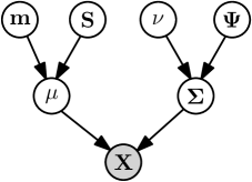
Figure 2: Graphical model for the Gibbs-filter/RTSS. ${\mathbf{X}}$ are data from a joint distribution, ${\boldsymbol{\mathbf{\mu}}}$ and ${\mathbf{\Sigma}}$ are the mean and the covariance of ${\mathbf{X}}$. The parameters of the conjugate priors on the mean and the covariance are denoted by ${\boldsymbol{\mathbf{m}}},{\mathbf{S}}$ and ${\mathbf{\Psi}},\nu$, respectively.

At each time step, we use Gibbs sampling to infer the moments of the joint distributions ${p}({\boldsymbol{\mathbf{x}}}_{t-1},{\boldsymbol{\mathbf{x}}}_{t}|{\boldsymbol{\mathbf{z}}}_{1:t-1})$ and ${p}({\boldsymbol{\mathbf{x}}}_{t},{\boldsymbol{\mathbf{z}}}_{t}|{\boldsymbol{\mathbf{z}}}_{1:t-1})$. Fig. 2 shows the graphical model for inferring the mean ${\boldsymbol{\mathbf{\mu}}}$ and the covariance ${\mathbf{\Sigma}}$ from the joint data set ${\mathbf{X}}$ using Gibbs sampling. The parameters of the conjugate priors on the mean ${\boldsymbol{\mathbf{\mu}}}$ and the covariance ${\mathbf{\Sigma}}$ are denoted by ${\boldsymbol{\mathbf{m}}},{\mathbf{S}}$ and ${\mathbf{\Psi}},\nu$, respectively.

To infer the moments of the joint ${p}({\boldsymbol{\mathbf{x}}}_{t-1},{\boldsymbol{\mathbf{x}}}_{t}|{\boldsymbol{\mathbf{z}}}_{1:t-1})$, we first generate i.i.d. samples from the filter distribution ${p}({\boldsymbol{\mathbf{x}}}_{t-1}|{\boldsymbol{\mathbf{z}}}_{1:t-1})$ and map them through the transition function $f$. The samples and their mappings serve as samples ${\mathbf{X}}$ from the joint distribution ${p}({\boldsymbol{\mathbf{x}}}_{t-1},{\boldsymbol{\mathbf{x}}}_{t}|{\boldsymbol{\mathbf{z}}}_{1:t-1})$. With a conjugate Gaussian prior $\mathcal{N}({\boldsymbol{\mathbf{\mu}}}\,|\,{\boldsymbol{\mathbf{m}}},{\mathbf{S}})$ on the joint mean, and a conjugate inverse Wishart prior distribution $\mathcal{IW}({\mathbf{\Sigma}}|{\mathbf{\Psi}},\nu)$ on the joint covariance matrix, we infer the posterior distributions on ${\boldsymbol{\mathbf{\mu}}}$ and ${\mathbf{\Sigma}}$. By sampling from these posterior distributions, we obtain unbiased estimates of the desired mean and the covariance of the joint ${p}({\boldsymbol{\mathbf{x}}}_{t-1},{\boldsymbol{\mathbf{x}}}_{t}|{\boldsymbol{\mathbf{z}}}_{1:t-1})$ as the sample average (after a burn in).

To infer the mean and the covariance of the joint ${p}({\boldsymbol{\mathbf{x}}}_{t},{\boldsymbol{\mathbf{z}}}_{t}|{\boldsymbol{\mathbf{z}}}_{1:t-1})$, we proceed similarly: We generate i.i.d. samples from the distribution ${p}({\boldsymbol{\mathbf{x}}}_{t}|{\boldsymbol{\mathbf{z}}}_{1:t-1})$, which are subsequently mapped through the measurement function. The combined data set of i.i.d. samples and their mappings define the joint data set ${\mathbf{X}}$. Again, we choose a conjugate Gaussian prior on the mean vector and a conjugate inverse Wishart prior on the covariance matrix of the joint ${p}({\boldsymbol{\mathbf{x}}}_{t},{\boldsymbol{\mathbf{z}}}_{t}|{\boldsymbol{\mathbf{z}}}_{1:t-1})$. Using Gibbs sampling, we sample means and covariances from the posteriors and obtain unbiased estimates for the mean and the covariance of the joint ${p}({\boldsymbol{\mathbf{x}}}_{t},{\boldsymbol{\mathbf{z}}}_{t}|{\boldsymbol{\mathbf{z}}}_{1:t-1})$.

Alg. 2 outlines the steps for computing the joint distribution ${p}({\boldsymbol{\mathbf{x}}}_{t},{\boldsymbol{\mathbf{z}}}_{t}|{\boldsymbol{\mathbf{z}}}_{1:t-1})$.

Algorithm 2 Inferring the mean ${\boldsymbol{\mathbf{\mu}}}_{x,z}$ and the covariance ${\mathbf{\Sigma}}_{x,z}$ of ${p}({\boldsymbol{\mathbf{x}}}_{t},{\boldsymbol{\mathbf{z}}}_{t}|{\boldsymbol{\mathbf{z}}}_{1:t-1})$ using Gibbs sampling

1:pass in marginal distribution ${p}({\boldsymbol{\mathbf{x}}}_{t}|{\boldsymbol{\mathbf{z}}}_{1:t-1})$, burn-in period $B$, number $L$ of Gibbs iterations, size $N$ of data set

2:init. conjugate priors on joint mean and covariance $\mathcal{N}({\boldsymbol{\mathbf{\mu}}}_{x,z}\,|\,{\boldsymbol{\mathbf{m}}},{\mathbf{S}})$ and $\mathcal{IW}({\mathbf{\Sigma}}_{x,z}|{\mathbf{\Psi}},\nu)$

3:${\mathbf{X}}\coloneqq[{\boldsymbol{\mathbf{x}}}_{t}^{(i)},g({\boldsymbol{\mathbf{x}}}_{t}^{(i)})+{\boldsymbol{\mathbf{v}}}_{t}^{(i)}]_{i=1}^{N}$ $\triangleright$ generate joint data set

4:sample ${\boldsymbol{\mathbf{\mu}}}_{1}\sim\mathcal{N}({\boldsymbol{\mathbf{m}}},{\mathbf{S}})$

5:sample ${\mathbf{\Sigma}}_{1}\sim\mathcal{I}W({\mathbf{\Psi}},\nu)$

6:for $j=1$ to $L$ do $\triangleright$ for $L$ Gibbs iterations do

7:     update ${\boldsymbol{\mathbf{m}}}|{\mathbf{X}},{\boldsymbol{\mathbf{\mu}}}_{j},{\mathbf{\Sigma}}_{j}$ $\triangleright$ posterior parameter (mean) of ${p}({\boldsymbol{\mathbf{\mu}}}_{j})$

8:     update ${\mathbf{S}}|{\mathbf{X}},{\boldsymbol{\mathbf{\mu}}}_{j},{\mathbf{\Sigma}}_{j}$ $\triangleright$ posterior parameter (covariance) of ${p}({\boldsymbol{\mathbf{\mu}}}_{j})$

9:     sample ${\boldsymbol{\mathbf{\mu}}}_{j+1}\sim\mathcal{N}({\boldsymbol{\mathbf{m}}},{\mathbf{S}})$ $\triangleright$ sample mean of the joint

10:     update ${\mathbf{\Psi}}|{\mathbf{X}},{\boldsymbol{\mathbf{\mu}}}_{j+1},{\mathbf{\Sigma}}_{j}$ $\triangleright$ posterior hyper-parameter (scale matrix) of ${p}({\boldsymbol{\mathbf{\Sigma}}}_{j})$

11:     update $\nu|{\mathbf{X}},{\boldsymbol{\mathbf{\mu}}}_{j+1},{\mathbf{\Sigma}}_{j}$ $\triangleright$ posterior hyper-parameter (degrees of freedom) of ${p}({\boldsymbol{\mathbf{\Sigma}}}_{j})$

12:     sample ${\mathbf{\Sigma}}_{j+1}\sim\mathcal{IW}({\mathbf{\Psi}},\nu)$ $\triangleright$ sample covariance of the joint

13:end for

14:${\boldsymbol{\mathbf{\mu}}}_{x,z}\coloneqq\mathds{E}[{\boldsymbol{\mathbf{\mu}}}_{B+1:L}]$ $\triangleright$ unbiased estimate of the mean of the joint distribution

15:${\mathbf{\Sigma}}_{x,z}\coloneqq\mathds{E}[{\mathbf{\Sigma}}_{B+1:L}]$ $\triangleright$ unbiased estimate of the covariance of the joint distribution

16:return ${\boldsymbol{\mathbf{\mu}}}_{x,z},{\mathbf{\Sigma}}_{x,z}$ $\triangleright$ return inferred mean and covariance of the joint

Since the chosen priors for the mean and the covariance are conjugate priors, all updates of the posterior hyper-parameters can be computed analytically [10].

The moments of ${p}({\boldsymbol{\mathbf{x}}}_{t-1},{\boldsymbol{\mathbf{x}}}_{t}|{\boldsymbol{\mathbf{z}}}_{1:t-1})$, which are required for smoothing, are computed similarly by exchanging the pass-in distributions and the mapping function.

5 Numerical Evaluation

As a proof of concept, we show that the Gibbs-RTSS proposed in Sec. 4.2 performs well in linear and nonlinear systems. As performance measures, we consider the expected root mean square error (RMSE) and the expected negative log-likelihood (NLL) per data point in the trajectory. For a single trajectory, the NLL is given by

NLL $$=-\frac{1}{T+1}\sum_{t=0}^{T}\log\mathcal{N}(x_{t}^{\text{truth}}|\mu_{t|\tau}^{x},(\sigma_{t|\tau}^{x})^{2})\,,$$ (33)

where $\tau=t$ for filtering and $\tau=T$ for smoothing. While the RMSE solely penalizes the distance of the true state and the mean of the filtering/smoothing distribution, the NLL measures the coherence of the filtering/smoothing distributions, i.e., the NLL values are high if $x_{t}^{\text{truth}}$ is an unlikely observation under ${p}(x_{t}|\mu_{t|\tau}^{x},(\sigma_{t|\tau}^{x})^{2})$, $\tau\in\{t,T\}$. In our experiments, we chose a time horizon $T=50$.

5.1 Proof of Concept: Linear System

First, we tested the performance of the Gibbs-filter/RTSS in the linear system

$$x_{t} =x_{t-1}+w_{t}$$ (34)

$$z_{t} =-2\,x_{t}+v_{t}\,,$$ (35)

where $w_{t}\sim\mathcal{N}(0,1),v_{t}\sim\mathcal{N}(0,10),p(x_{0})=\mathcal{N}(0,5)$. In a linear system, the (E)KF is optimal and unbiased [1]. The Gibbs-filter/RTSS perform as well as the EKF/EKS as shown in Fig. 3, which shows the expected performances (with the corresponding standard errors) of the filters/smoothers over 100 independent runs, where $x_{0}\sim{p}(x_{0})$. The Gibbs-sampler parameters were set to $(N,L,B)=(1000,200,100)$, Alg. 2.

	EKF	Gibbs-filter⋆	EKS	Gibbs-RTSS⋆
RMSE	$1.11\pm 0.014$	$1.12\pm 0.014$	$0.88\pm 0.011$	$0.89\pm 0.011$
NLL	$1.52\pm 0.012$	$1.52\pm 0.012$	$1.30\pm 0.013$	$1.30\pm 0.012$

Figure 3: Expected performances (linear system) with standard error of the mean. The results obtained from the optimal linear algorithm and the Gibbs-filter/RTSS are nearly identical.

5.2 Nonlinear System: Non-stationary Growth Model

As a nonlinear example, we consider the dynamic system

$$x_{t} =\tfrac{x_{t-1}}{2}+\tfrac{25x_{t-1}}{1+x_{t-1}^{2}}+8\cos(1.2\,(t-1))+w_{t}\,,$$ (36)

$$z_{t} =\tfrac{x_{t}^{2}}{20}+v_{t}\,,$$ (37)

with exactly the same setup as in [8]: $w_{t}\sim\mathcal{N}(0,1)$, $v_{t}\sim\mathcal{N}(0,10)$, and $p(x_{0})=\mathcal{N}(x_{0}|0,5)$. This system is challenging for Gaussian filters due to its quadratic measurement equation and its highly nonlinear system equation.

We run the Gibbs-RTSS, the EKS, the CKS, and the URTSS [21] for comparison. We chose the Gibbs parameters $(N,L,B)=(1000,200,100)$. For 100 independent runs starting from $x_{0}\sim{p}(x_{0})$, we report the expected RMSE and NLL performance measures in Fig. 4.

filters	Gibbs-filter⋆	EKF	CKF	UKF
RMSE	$\mathbf{5.04\pm 0.088}$	$11.1\pm 0.29$	$6.18\pm 0.17$	$8.57\pm 0.16$
NLL	$\mathbf{2.87\pm 0.12}$	$26.1\pm 1.18$	$9.96\pm 0.75$	$13.6\pm 0.68$
smoothers	Gibbs-RTSS⋆	EKS	CKS⋆	URTSS
RMSE	$\mathbf{4.01\pm 0.085}$	$10.6\pm 0.28$	$5.66\pm 0.20$	$8.02\pm 0.16$
NLL	${\bf{{\color[rgb]{0.2,0.6,0.2}2.78\pm 0.15}}}$	${\bf{{\color[rgb]{1,0,0}90.6\pm 10.3}}}$	${\bf{{\color[rgb]{1,0,0}28.9\pm 3.31}}}$	${\bf{{\color[rgb]{1,0,0}16.3\pm 0.16}}}$

Figure 4: Expected performances (nonlinear system) with standard error of the mean. The Gibbs-RTSS is the only coherent smoother, i.e., it improves the filtering results in the NLL measure.

Both high expected NLL-values and the fact that smoothing makes them even higher hint at the incoherencies of the EKF/EKS, the CKF/CKS, and the UKF/URTSS. The Gibbs-RTSS was the only considered smoother that consistently improved the results of the filtering step. Therefore, we conclude that the Gibbs-filter/RTSS is coherent.

Fig. 5 shows example realizations of filtering and smoothing using the Gibbs-filter/RTSS, the EKF/EKS, the CKF/CKS, and the UKF/URTSS, respectively.

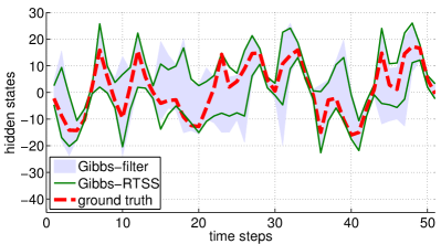
(a) Gibbs-filter (Gibbs-RTSS). RMSE: 5.56 (4.18), NLL: 2.65 (2.45).

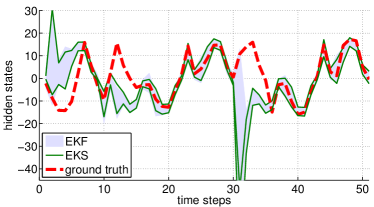
(b) EKF (EKS). RMSE: 11.3 (14.7), NLL: 16.5 (20.8).

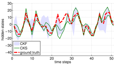
(c) CKF (CKS). RMSE: 5.66 (5.96), NLL: 7.32 (20.7).

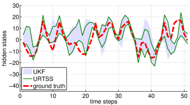
(d) UKF (URTSS). RMSE: 7.87 (7.18), NLL: 8.66 (9.93).

Figure 5: Example trajectories of filtering/smoothing in the nonlinear growth model using 5(a) Gibbs-RTSS, 5(b) EKS, 5(c) CKS, 5(d) URTSS. The filter distributions are represented by the shaded areas ($95\%$ confidence area), the smoothing distributions are shown by solid green lines ($95\%$ confidence area). The actual realization of the latent state is the dashed red graph.

The Gibbs-filter/RTSS appropriately inferred the variances of the latent state while the other filters/smoothers did not (neither of them is moment-preserving), which can lead to incoherent filtering/smoothing distributions [5], see also Fig. 4.

6 Discussion

Our Gibbs-filter/RTSS differs from [4], where Gibbs sampling is used to infer the noise in a linear system. Instead, we infer the means and covariances of the full joint distributions ${p}({\boldsymbol{\mathbf{x}}}_{t-1},{\boldsymbol{\mathbf{x}}}_{t}|{\boldsymbol{\mathbf{z}}}_{1:t-1})$ and ${p}({\boldsymbol{\mathbf{x}}}_{t},{\boldsymbol{\mathbf{z}}}_{t}|{\boldsymbol{\mathbf{z}}}_{1:t-1})$ in nonlinear systems from data. Neither the Gibbs-filter nor the Gibbs-RTSS require to know the noise matrices ${\mathbf{R}},{\mathbf{Q}}$, but they can be inferred as a part of the joint distributions if access to the dynamic system is given. Unlike the Gaussian particle filter [14], the proposed Gibbs-filter is not a particle filter. Therefore, it does not suffer from degeneracy due to importance sampling.

Although the Gibbs-filter is computationally more involved than the EKF/UKF/CKF, it can be used as a baseline method to evaluate the accuracy and coherence of more efficient algorithms: When using sufficiently many samples the Gibbs-filter can be considered a close approximation to a moment-preserving filter in nonlinear stochastic systems.

The sampling approach to inferring the means and covariances of two joint distributions proposed in this paper can be extended to infer the means and covariances of a single joint, namely, ${p}({\boldsymbol{\mathbf{x}}}_{t-1},{\boldsymbol{\mathbf{x}}}_{t},{\boldsymbol{\mathbf{z}}}_{t}|{\boldsymbol{\mathbf{z}}}_{1:t-1})$. This would increase the dimensionality of the parameters to be inferred, but it would remove slight inconsistencies that appear in the present approach: Ideally, the marginals ${p}({\boldsymbol{\mathbf{x}}}_{t}|{\boldsymbol{\mathbf{z}}}_{1:t-1})$, i.e., the time update, which can be obtained from both joints ${p}({\boldsymbol{\mathbf{x}}}_{t-1},{\boldsymbol{\mathbf{x}}}_{t}|{\boldsymbol{\mathbf{z}}}_{1:t-1})$ and ${p}({\boldsymbol{\mathbf{x}}}_{t},{\boldsymbol{\mathbf{z}}}_{t}|{\boldsymbol{\mathbf{z}}}_{1:t-1})$ are identical. Due to the finite number of samples, small errors are introduced. In our experiments, they were small, i.e., the relative difference error was smaller than $10^{-5}$. Using the joint ${p}({\boldsymbol{\mathbf{x}}}_{t-1},{\boldsymbol{\mathbf{x}}}_{t},{\boldsymbol{\mathbf{z}}}_{t}|{\boldsymbol{\mathbf{z}}}_{1:t-1})$ would avoid this kind of error.

The Gibbs-filter/RTSS only need to be able to evaluation the system and measurement functions. No further requirements such as differentiability are needed. A similar procedure for MCMC-based smoothing is applicable when, instead of Gibbs sampling, slice sampling [18] or elliptical slice sampling [17] is used, potentially combined with GPs that model the functions $f$ and $g$.

The Gibbs-RTSS code is publicly available at mloss.org.

In the context of Gaussian process dynamic systems, the GP-EKF, the GP-UKF [13], and the GP-ADF [6] can directly be extended to smoothers using the results from this paper. The GP-URTSS (smoothing extension of the GP-UKF) and the GP-RTSS (smoothing extension of the GP-ADF) are presented in [5].

7 Conclusion

Using a general probabilistic perspective on Gaussian filtering and smoothing, we first showed that it is sufficient to determine Gaussian approximations to two joint probability distributions to perform Gaussian filtering and smoothing. Computational approaches to Gaussian filtering and Rauch-Tung-Striebel smoothing can be distinguished by their respective methods used to determining two joint distributions.

Second, our results allow for a straightforward derivation and implementation of novel Gaussian filtering and smoothing algorithms, e.g., the cubature Kalman smoother. Additionally, we presented a filtering smoothing algorithm based on Gibbs sampling as an example. Our experimental results show that the proposed Gibbs-filter/Gibbs-RTSS compares well with state-of-the-art Gaussian filters and RTS smoothers in terms of robustness and accuracy.

Acknowledgements

The authors thank S. Mohamed, P. Orbanz, M. Krainin, and D. Fox for valuable suggestions and discussions. MPD has been supported by ONR MURI grant N00014-09-1-1052 and by Intel Labs. HO has been partially supported by the Swedish foundation for strategic research in the center MOVIII and by the Swedish Research Council in the Linnaeus center CADICS.

References

- [1] Brian D. O. Anderson and John B. Moore. Optimal Filtering. Dover Publications, Mineola, NY, USA, 2005.
- [2] Ienkaran Arasaratnam and Simon Haykin. Cubature Kalman Filters. IEEE Transactions on Automatic Control, 54(6):1254–1269, 2009.
- [3] Christopher M. Bishop. Pattern Recognition and Machine Learning. Information Science and Statistics. Springer-Verlag, 2006.
- [4] Christopher K. Carter and Robert Kohn. On Gibbs Sampling for State Space Models. Biometrika, 81(3):541–553, August 1994.
- [5] Marc P. Deisenroth. Efficient Reinforcement Learning using Gaussian Processes, volume 9 of Karlsruhe Series on Intelligent Sensor-Actuator-Systems. KIT Scientific Publishing, November 2010. ISBN 978-3-86644-569-7.
- [6] Marc P. Deisenroth, Marco F. Huber, and Uwe D. Hanebeck. Analytic Moment-based Gaussian Process Filtering. In L. Bouttou and M. L. Littman, editors, Proceedings of the 26th International Conference on Machine Learning, pages 225–232, Montreal, QC, Canada, June 2009. Omnipress.
- [7] Marc P. Deisenroth and Henrik Ohlsson. A General Perspective on Gaussian Filtering and Smoothing: Explaining Current and Deriving New Algorithms. In Proccedings of the American Control Conference, 2011. accepted for publication.
- [8] Arnaud Doucet, Simon J. Godsill, and Christophe Andrieu. On Sequential Monte Carlo Sampling Methods for Bayesian Filtering. Statistics and Computing, 10:197–208, 2000.
- [9] Stuart Geman and Donald Geman. Stochastic Relaxation, Gibbs Distributions, and the Bayesian Restoration of Images. IEEE Transactions on Pattern Analysis and Machine Intelligence, 6(6):721–741, 1984.
- [10] Walter R. Gilks, Sylvia Richardson, and David J. Spiegelhalter, editors. Markov Chain Monte Carlo in Practice: Interdisciplinary Statistics. Chapman & Hall, 1996.
- [11] Simon J. Julier and Jeffrey K. Uhlmann. Unscented Filtering and Nonlinear Estimation. Proceedings of the IEEE, 92(3):401–422, March 2004.
- [12] Rudolf E. Kalman. A New Approach to Linear Filtering and Prediction Problems. Transactions of the ASME — Journal of Basic Engineering, 82(Series D):35–45, 1960.
- [13] Jonathan Ko and Dieter Fox. GP-BayesFilters: Bayesian Filtering using Gaussian Process Prediction and Observation Models. Autonomous Robots, 27(1):75–90, July 2009.
- [14] Jayesh H. Kotecha and Petar M. Djuric. Gaussian Particle Filtering. IEEE Transactions on Signal Processing, 51(10):2592–2601, October 2003.
- [15] Peter S. Maybeck. Stochastic Models, Estimation, and Control, volume 141 of Mathematics in Science and Engineering. Academic Press, Inc., 1979.
- [16] Thomas P. Minka. From Hidden Markov Models to Linear Dynamical Systems. Technical Report TR 531, Massachusetts Institute of Technology, 1998.
- [17] Iain Murray, Ryan P. Adams, and David J.C. MacKay. Elliptical Slice Sampling. In Y. W. Teh and M. Titterington, editors, Proceedings of the 13th International Conference on Artificial Intelligence and Statistics, JMLR: W&CP 9, pages 541–548, 2010.
- [18] Radford M. Neal. Slice Sampling. Annals of Statistics, 31(3):705–767, 2003.
- [19] H. E. Rauch, F. Tung, and C. T. Striebel. Maximum Likelihood Estimates of Linear Dynamical Systems. AIAA Journal, 3:1445–1450, 1965.
- [20] Sam Roweis and Zoubin Ghahramani. A Unifying Review of Linear Gaussian Models. Neural Computation, 11(2):305–345, 1999.
- [21] Simo Särkkä. Unscented Rauch-Tung-Striebel Smoother. IEEE Transactions on Automatic Control, 53(3):845–849, 2008.
- [22] Sebastian Thrun, Wolfram Burgard, and Dieter Fox. Probabilistic Robotics. The MIT Press, Cambridge, MA, USA, 2005.