$\zeta$-regularised spectral determinants on metric graphs

Abstract

Several general results for the spectral determinant of the Schrödinger operator on metric graphs are reviewed. Then, a simple derivation for the $\zeta$-regularised spectral determinant is proposed, based on the Roth trace formula. Two types of boundary conditions are studied : functions continuous at the vertices and functions whose derivative is continuous at the vertices. The $\zeta$-regularised spectral determinant of the Schrödinger operator acting on functions with the most general boundary conditions is conjectured in conclusion. The relation to the Ihara, Bass and Bartholdi formulae obtained for combinatorial graphs is also discussed.

^(a) Univ. Paris Sud ; CNRS ; LPTMS, UMR 8626, Bât. 100, F-91405 Orsay, France.

^(b) Univ. Paris Sud ; CNRS ; LPS, UMR 8502, Bât. 510, F-91405 Orsay, France.

PACS numbers : 02.70.Hm ; 02.10.Ox

1 Introduction

Spectral determinants (i.e. $\zeta$-functions or $L$-functions) and trace formulae in graphs have attracted a lot of interest in the mathematical literature [22, 34, 35, 20, 21, 3, 15, 37, 2, 5, 17, 25, 19] and in the physical literature as well [32, 33, 4, 26, 1, 10, 11, 6, 23, 14, 42, 7]. In this article we will consider the case of the Laplace $-\Delta$ or the Schrödinger operator $-\Delta+V(x)$ on a metric graph. We denote by $\{E_{n}\}$ the spectrum of the operator $-\Delta+V(x)$, and introduce the spectral determinant by the formal definition

$$S(\gamma)=\det[\gamma-\Delta+V(x)]=\prod_{n}(\gamma+E_{n})\>,$$ (1)

where $\gamma$ is some “spectral parameter”. This object was shown to be a very convenient quantity in order to study several questions in metric graphs, like various properties of the Brownian motion [10, 11, 6, 42, 7] or transport and magnetic properties of networks of metallic wires [32, 33, 1, 14].

Because the operator $-\Delta+V(x)$ acts in a space of infinite dimension, the computation of the spectral determinant (1) requires in practice some regularisation. Starting from the trace of the Green function, i.e. the Laplace transform of the partition function $Z(t)=\sum_{n}{\mbox{\large e}}^{-tE_{n}}$,

$$G(\gamma)=\sum_{n}\frac{1}{\gamma+E_{n}}=\int_{0}^{\infty}{\rm d}{}t\,Z(t)\,{\mbox{\large e}}^{-\gamma{}t}\>,$$ (2)

furnishes a first possible regularisation, used in Refs. [32, 33, 1, 8, 10, 42, 7, 44]. Performing some integration with respect to the spectral parameter we obtain

$$S^{\mathrm{GF}}(\gamma)\stackrel{{\scriptstyle\mbox{\tiny def}}}{{=}}\exp\int_{\gamma_{0}}^{\gamma}{\rm d}\gamma^{\prime}\,G(\gamma^{\prime})=S(\gamma)/S(\gamma_{0})$$ (3)

For example, consider the Laplace operator on a line $[0,L]$ with Neumann boundary conditions. The spectrum is in this case $E_{n}=(n\pi/L)^{2}$ with $n\in\mathbb{N}$ and we obtain $S^{\mathrm{GF}}(\gamma)=\frac{\sqrt{\gamma}\sinh\sqrt{\gamma}{}L}{\sqrt{\gamma}_{0}\sinh\sqrt{\gamma}_{0}{}L}$. This procedure however leaves some arbitrary in the choice of the parameter $\gamma_{0}$.

Another well known regularisation for determinants is the $\zeta$-regularisation whose starting point is to introduce the $\zeta$-function

$$\zeta(s,\gamma)\stackrel{{\scriptstyle\mbox{\tiny def}}}{{=}}\sum_{n}{(\gamma+E_{n})^{-s}}=\frac{1}{\Gamma(s)}\int_{0}^{\infty}{\rm d}{}t\,t^{s-1}\,{\mbox{\large e}}^{-\gamma t}\,Z(t)\>,$$ (4)

that we have expressed as a Mellin transform of the partition function, for convenience for the following discussion. Note that $\zeta(1,\gamma)=G(\gamma)$. The $\zeta$-regularised determinant is then related to a derivative of the $\zeta$-function :

$$S^{\zeta}(\gamma)\stackrel{{\scriptstyle\mbox{\tiny def}}}{{=}}\exp-\frac{\mathrm{d}\zeta}{\mathrm{d}s}(0,\gamma)\>.$$ (5)

In this case no arbitrary is left within the calculation of the determinant. Coming back to the simple example considered above of the Laplace operator on a line $[0,L]$ with Neumann boundary conditions, we get in this case $S^{\zeta}(\gamma)=2\sqrt{\gamma}\sinh\sqrt{\gamma}{}L$ (derived below).

An important remark is that various regularisations only differ by some $\gamma$-independent prefactors. This explains why the choice of the regularisation has no consequence on the properties studied in Refs. [32, 33, 1, 10, 11, 6, 14, 42, 7] since they are always related to derivatives of $\ln{}S(\gamma)$, with respect to the spectral parameter $\gamma$ or other parameters. In a recent work [44] some procedure was proposed in order to construct the spectral determinant of a graph by combinations of the determinants of subgraphs. In this case it is crucial to define precisely the prefactor of the spectral determinant.

In a recent paper [17], Friedlander has derived the $\zeta$-regularised determinant for the Schrödinger operator on a metric graph. One should also mention that the analysis of the regularised determinant of the Laplace operator for general boundary conditions, $\det^{\prime}(-\Delta)$ with the prime indicating exclusion of zero mode contribution is there is some, was the subject of the very recent work [19]. It is the purpose of the present article to propose another derivation of the $\zeta$-regularised determinant for the Schrödinger operator $\det[\gamma-\Delta+V(x)]$. Our approach is based on the Roth trace formula [34] and will allow simple extension of Friedlander’s result to other choices of boundary conditions at the vertices.

In the next section we set notations. In section 3 we mostly recall some known general results obtained by Desbois in Ref. [10] and needed for the following sections. The section 4 focuses on the case of functions continuous at the vertices and section 5 on the case of functions with derivative continuous at vertices. The $\zeta$-regularisation of the spectral determinant is provided in section 6.

2 Metric graphs and Laplace operator

A graph is a set of $V$ vertices (here labelled with greek letters $\alpha$, $\beta$,…) linked by $B$ bonds (denoted as $({\alpha\beta})$,…). Each bond $({\alpha\beta})$ is associated to two arcs (oriented bonds) ${\alpha\beta}$ and ${\beta\alpha}$ (arc will be also labelled with roman indices $a$, $b$,….). For the arc $a=\alpha\beta$, the reversed arc is denoted $\bar{a}=\beta\alpha$. We introduce the adjacency matrix : $a_{\alpha\beta}=1$ if $\alpha$ is linked to $\beta$ by a bond and $a_{\alpha\beta}=0$ otherwise. We denote by $m_{\alpha}=\sum_{\beta}{}a_{\alpha\beta}$ the coordination number (valency) of the vertex. The graph is said to be a metric graph (or a quantum graph) if each bond is identified with a finite interval $(0,l_{\alpha\beta})\in\mathbb{R}$, where $l_{\alpha\beta}$ designates the length of the bond linking the vertices $\alpha$ and $\beta$. In this case we may consider a scalar function $\psi(x)$, characterised by a set of $B$ components $\psi_{\alpha\beta}(x_{\alpha\beta})$ with $x_{\alpha\beta}\in(0,l_{\alpha\beta})$. The component is labelled by the arc in order to specify the direction along which the coordinate is measured [this redundancy of the notation implies the obvious relation $\psi_{\alpha\beta}(x_{\alpha\beta})=\psi_{\beta\alpha}(x_{\beta\alpha})=\psi_{\beta\alpha}(l_{\alpha\beta}-x_{\alpha\beta})$].

Having introduced scalar functions living on the graph we may define the action of the Laplace operator $\Delta$ on such functions. Along a wire it acts as the usual second derivative $(\Delta\psi)_{\alpha\beta}(x)=\frac{\mathrm{d}^{2}}{\mathrm{d}x^{2}}\psi_{\alpha\beta}(x)$. At the vertices, the set of functions on which $\Delta$ acts must satisfy some boundary conditions in order to ensure self adjointness of the operator. Let us denote by $\psi(0)$ and $\psi^{\prime}(0)$ the vectors of size $2B$ gathering the values taken by the components and the derivatives at the vertices $\psi_{\alpha\beta}(0)$ and $\psi^{\prime}_{\alpha\beta}(0)$, respectively. The most general boundary conditions ensuring self adjointness of $\Delta$ are of the form

$$C\,\psi(0)+D\,\psi^{\prime}(0)=0\>,$$ (6)

where the $2B\times 2B$ matrices $C$ and $D$ satisfy (i) $CD^{\dagger}=DC^{\dagger}$. (ii) The $2B\times 4B$ matrix $(C,D)$ has maximal rank (equal to $2B$) [24]. Note that, characterising what arc is connected to what other arc, these two matrices encode all the information on the topology of the graph.

3 General results for the spectral determinant

In this section we mostly recall some results obtained by Desbois [10] for the spectral determinant of the Schrödinger operator for general boundary conditions. We compute the spectral determinant by constructing the Green function $\mathcal{G}(x,y)\stackrel{{\scriptstyle\mbox{\tiny def}}}{{=}}\langle\kern 1.29167ptx\kern 1.29167pt|\frac{1}{\gamma-{\rm D}_{x}^{2}+V(x)}|\kern 1.29167pty\kern 1.29167pt\rangle$, where ${\rm D}_{x}\stackrel{{\scriptstyle\mbox{\tiny def}}}{{=}}\frac{\mathrm{d}}{\mathrm{d}x}-{\rm i}{}A(x)$ is the covariant derivative. Note that the replacement of $\Delta$ by ${\rm D}_{x}^{2}$ is motivated by physical considerations [31, 1, 39]. It might also be useful in order to study winding properties of Brownian curves in the graph [42, 7]. It will affect calculations in a very simple manner through the introduction of additional (magnetic) phases. In the following it will be understood that the $2B$-vector $\psi^{\prime}(0)$ of Eq. (6) gathers the covariant derivatives.

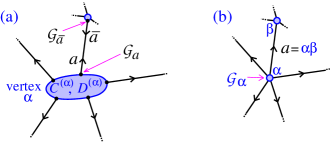
Figure 1: The vertex $\alpha$. (a) For general boundary conditions, matching of the Green function at the vertex is described through two matrices $m_{\alpha}\times m_{\alpha}$ denoted $C^{(\alpha)}$ and $D^{(\alpha)}$ (the blocks of the matrices $C$ and $D$). One must assign a value of the Green function $\mathcal{G}_{a}$ to each arc $a$. (b) For continuous boundary condition at the vertex, the matrices $C^{(\alpha)}$ and $D^{(\alpha)}$ take the form (29). In this case one can assign to each vertex $\alpha$ a single “vertex variable” $\mathcal{G}_{\alpha}$.

3.1 Arc determinant (1)

Let us consider two points $x$ and $y$ belonging to the two arcs $a$ and $b$, respectively. On the arc $a$ we use the set of independent solutions $f_{a}$ and $f_{\bar{a}}$ of the differential equation $[\gamma-\frac{\mathrm{d}^{2}}{\mathrm{d}x^{2}}+V_{a}(x)]f(x)=0$ such that $f_{a}(0)=1$ and $f_{a}(l_{a})=0$ (see appendix A). The Green function depends on two coordinates $x$ and $y$ and therefore on must specify by two indices (here $a$ and $b$) to which arcs they belong to :

$$\mathcal{G}_{a,b}(x_{a},y_{b})= \mathcal{G}_{a}\,f_{a}(x_{a})\,{\mbox{\large e}}^{{\rm i}A_{a}x_{a}}+\mathcal{G}_{\bar{a}}\,f_{\bar{a}}(x_{\bar{a}})\,{\mbox{\large e}}^{{\rm i}A_{\bar{a}}x_{\bar{a}}}$$

$$+\delta_{(a),(b)}\frac{{\mbox{\large e}}^{{\rm i}A_{a}(x_{a}-y_{a})}}{{W}_{a}}\>f_{a}(\mathop{\mathrm{max}}\nolimits\left(x_{a},y_{a}\right))\>f_{\bar{a}}(\mathop{\mathrm{max}}\nolimits\left(x_{\bar{a}},y_{\bar{a}}\right))\>,$$ (7)

where $\mathcal{G}_{a}$ and $\mathcal{G}_{\bar{a}}$ denote the values of the Green function at the two ends of the bond $(a)$ (see figure 1.a). We have introduce the notation $\delta_{(a),(b)}\stackrel{{\scriptstyle\mbox{\tiny def}}}{{=}}\delta_{a,b}+\delta_{a,\bar{b}}$. Note that the dependence of $\mathcal{G}_{a}$ and $\mathcal{G}_{\bar{a}}$ in the coordinate $y$ is implicit. $A_{a}=A(x)$ for $x\in(a)$ is the (constant) vector potential on the bond  and $\theta_{a}=A_{a}l_{a}$ the magnetic flux along the wire. ${W}_{a}=-f^{\prime}_{a}(l_{a})$ is the Wronski determinant of the two linearly independent solutions, Eq. (69). All the values of the Green function at the vertices $\mathcal{G}_{a,b}(0,y_{b})=\mathcal{G}_{a}$ (figure 1.a) are gathered in the vector $\mathcal{G}(0)$ of size $2B$ and all covariant derivatives $({\rm D}_{x}\mathcal{G})_{a,b}(0,y_{b})$ in the vector $\mathcal{G}^{\prime}(0)$. We obtain

$$\mathcal{G}^{\prime}(0)=M\,\mathcal{G}(0)+\left(\begin{array}[]{cccccc}\vdots\\ 0\\ f_{b}(y_{b})\,{\mbox{\large e}}^{-{\rm i}A_{b}y_{b}}\\ f_{\bar{b}}(y_{\bar{b}})\,{\mbox{\large e}}^{-{\rm i}A_{\bar{b}}y_{\bar{b}}}\\ 0\\ \vdots\end{array}\right)\begin{array}[]{cccccc}\phantom{\vdots}\\ \phantom{0}\\ \leftarrow b\\ \leftarrow\bar{b}\\ \phantom{0}\\ \phantom{\vdots}\end{array}$$ (8)

where the matrix $M$ couples an arc $a$ to itself and to the reversed arc $\bar{a}$ :

$$M_{a,b}\stackrel{{\scriptstyle\mbox{\tiny def}}}{{=}}\delta_{a,b}\,f^{\prime}_{a}(0)-\delta_{a,\bar{b}}\,f^{\prime}_{\bar{a}}(l_{a})\,{\mbox{\large e}}^{{\rm i}\theta_{\bar{a}}}\>.$$ (9)

Noticing that $f^{\prime}_{\bar{a}}(l_{a})=f^{\prime}_{a}(l_{a})\in\mathbb{R}$ (see appendix A) and $\theta_{\bar{a}}=-\theta_{a}$ shows that this matrix is Hermitian. Imposing boundary conditions at vertices, $C\,\mathcal{G}(0)+D\,\mathcal{G}^{\prime}(0)=0$, we obtain all values $\mathcal{G}_{a}$, that could be reinjected into Eq. (3.1). The Green function at coinciding points reads :

$$\mathcal{G}_{a,a}(x_{a},x_{a}) =-\left[(C+DM)^{-1}D\right]_{aa}\,f_{a}^{2}-\left[(C+DM)^{-1}D\right]_{a\bar{a}}\,f_{a}f_{\bar{a}}{\mbox{\large e}}^{{\rm i}\theta_{a}}$$

$$-\left[(C+DM)^{-1}D\right]_{\bar{a}a}\,f_{a}f_{\bar{a}}{\mbox{\large e}}^{{\rm i}\theta_{\bar{a}}}-\left[(C+DM)^{-1}D\right]_{\bar{a}\bar{a}}\,f_{\bar{a}}^{2}+\frac{1}{{W}_{a}}f_{a}f_{\bar{a}}$$ (10)

Integration over the Graph may be decomposed as integration over the bonds : $\int_{\mathrm{Graph}}{\rm d}{}x\,\mathcal{G}(x,x)=\sum_{(a)}\int_{0}^{l_{a}}{\rm d}{}x_{a}\,\mathcal{G}_{a,a}(x_{a},x_{a})$. The integration of product of functions $f_{a}$ and $f_{\bar{a}}$ is given by eqs. (71,72), hence

$$G(\gamma)=\int_{\mathrm{Graph}}{\rm d}{}x\,\mathcal{G}(x,x)=\mathop{\mathrm{Tr}}\nolimits\left\{(C+DM)^{-1}D\,\partial_{\gamma}M\right\}-\partial_{\gamma}\sum_{(a)}\ln[-f^{\prime}_{a}(l_{a})]\>,$$ (11)

where the trace runs over the $2B$ arc indices. Up to now, nothing has be assumed on the nature of the boundary conditions. An expansion of the trace provides a trace formula for $\int_{\mathrm{Graph}}{\rm d}{}x\,\mathcal{G}(x,x)$, where the expansion is interpreted as sum of contributions over cycles (orbits) in the graph.

We now suppose that the matrices $C$ and $D$ do not depend on the spectral parameter $\gamma$. Performing and integration $\ln S(\gamma)=\int^{\gamma}{\rm d}\gamma^{\prime}\,G(\gamma^{\prime})$, we obtain the first important result of Desbois :

$$\boxed{S(\gamma)=(-1)^{V}\prod_{(a)}\frac{-1}{f^{\prime}_{a}(l_{a})}\>\det(C+DM)}$$ (12)

where the product runs over the $B$ bonds. This provides a general expression of the spectral determinant in terms of $2B\times 2B$-matrices coupling arcs. We repeat that the matrix $M$ couples reversed arcs and contains local information related to the potential on each bound. On the other hand, the matrices $C$ and $D$, characterising which arcs arrive and issue from the vertices, encode the information on the topology of the graph. Note that the structure $\det(C+DM)$ was also obtained in [19] in the absence of the potential where the determinant $\det^{\prime}(-\Delta)$ was analysed (the prime indicates exclusion of zero mode). When $V(x)=0$ the matrix $M$ takes the form $M_{a,b}=-\sqrt{\gamma}\big{(}\delta_{a,b}\,\coth\sqrt{\gamma}l_{a}-\delta_{a,\bar{b}}\,\frac{1}{\sinh\sqrt{\gamma}l_{a}}\,{\mbox{\large e}}^{{\rm i}\theta_{\bar{a}}}\big{)}$.

The prefactor in Eq. (12) has been chosen arbitrarily and for convenience for the following. We will come back to the question of the prefactor in the section 6.

Limit $\gamma\to\infty$

For large positive spectral parameter we can ignore the potential, therefore $f_{a}^{\prime}(0)\simeq-\sqrt{\gamma}$ and $f_{a}^{\prime}(l_{a})\simeq-\sqrt{\gamma}{\mbox{\large e}}^{-\sqrt{\gamma}\,l_{a}}$. Hence the matrix $M$ becomes diagonal : $M_{a,b}\simeq-\delta_{a,b}\sqrt{\gamma}$ and we obtain

$$S(\gamma)\underset{\gamma\to+\infty}{\simeq}(-1)^{V}2^{-B}\gamma^{-B/2}{\mbox{\large e}}^{\sqrt{\gamma}\,\mathcal{L}}\>\det(C-\sqrt{\gamma}\,D)$$ (13)

where $\mathcal{L}=\sum_{(a)}l_{a}$ is the “total length” of the graph.

Example

Let us consider a ring of perimeter $L$ pierced by a magnetic flux $\theta$ (a graph in which the number of vertices can be reduced to $V=1$ with $B=1$ bond). We denote by $1$ and $\bar{1}$ the two reversed arcs. Let us consider boundary conditions described by the matrices given below by Eq. (29). We obtain

$$S(\gamma)=\frac{\lambda-f_{1}^{\prime}(0)-f_{\bar{1}}^{\prime}(0)+2f_{1}^{\prime}(L)\,\cos\theta}{-f_{1}^{\prime}(L)}\>.$$ (14)

It is interesting to point that this formula has found a practical physical application for a potential of the form $V(x)\propto{}x(L-x)$ in the context of the study of decoherence by electron-electron interaction in a phase coherent metallic ring [43] (hence $f_{1}(x)$ is a Hermite function and $f_{\bar{1}}(x)=f_{1}(L-x)$ due to the property $V(x)=V(L-x)$).

The case $V(x)=0$ is analysed in section 6.

3.2 Arc determinant (2)

The above derivation has privileged the use of variables $\mathcal{G}_{a}$ giving the value of the Green function at the vertices. Another natural choice is to deal with (covariant) derivatives of the Green function at the vertices. We write

$$\mathcal{G}_{a,b}(x_{a},y_{b})= \mathcal{G}^{\prime}_{a}\,g_{a}(x_{a})\,{\mbox{\large e}}^{{\rm i}A_{a}x_{a}}+\mathcal{G}^{\prime}_{\bar{a}}\,g_{\bar{a}}(x_{\bar{a}})\,{\mbox{\large e}}^{{\rm i}A_{\bar{a}}x_{\bar{a}}}$$

$$+\delta_{(a),(b)}\frac{{\mbox{\large e}}^{{\rm i}A_{a}(x_{a}-y_{a})}}{{W}^{g}_{a}}\>g_{a}(\mathop{\mathrm{max}}\nolimits\left(x_{a},y_{a}\right))\>g_{\bar{a}}(\mathop{\mathrm{max}}\nolimits\left(x_{\bar{a}},y_{\bar{a}}\right))$$ (15)

where the functions $g_{a}$ and $g_{\bar{a}}$ are solutions of the Schrödinger equation on the bond $(a)$ for fixed values of the derivative at the boundaries, $g^{\prime}_{a}(0)=1$ and $g^{\prime}_{a}(l_{a})=0$ (see appendix A). Following the lines of the previous subsection, we obtain

$$\mathcal{G}(0)=N\,\mathcal{G}^{\prime}(0)-\left(\begin{array}[]{cccccc}\vdots\\ 0\\ g_{b}(y_{b})\,{\mbox{\large e}}^{-{\rm i}A_{b}y_{b}}\\ g_{\bar{b}}(y_{\bar{b}})\,{\mbox{\large e}}^{-{\rm i}A_{\bar{b}}y_{\bar{b}}}\\ 0\\ \vdots\end{array}\right)\begin{array}[]{cccccc}\phantom{\vdots}\\ \phantom{0}\\ \leftarrow b\\ \leftarrow\bar{b}\\ \phantom{0}\\ \phantom{\vdots}\end{array}$$ (16)

where we have introduced the arc matrix

$$N_{a,b}\stackrel{{\scriptstyle\mbox{\tiny def}}}{{=}}\delta_{a,b}\,g_{a}(0)+\delta_{a,\bar{b}}\,g_{\bar{a}}(l_{a})\,{\mbox{\large e}}^{{\rm i}\theta_{\bar{a}}}\>.$$ (17)

Imposing the boundary conditions at the vertices we obtain the values $\mathcal{G}^{\prime}_{a}$. Reinjecting these expressions in Eq. (3.2), integration over the coordinate and summation over bonds give another general trace formula for the Green function

$$G(\gamma)=\int_{\mathrm{Graph}}{\rm d}{}x\,\mathcal{G}(x,x)=\mathop{\mathrm{Tr}}\nolimits\left\{(CN+D)^{-1}C\,\partial_{\gamma}N\right\}-\partial_{\gamma}\sum_{(a)}\ln[-g_{a}(l_{a})]\>.$$ (18)

For $\gamma$-independent matrices $C$ and $D$, integration over the spectral parameter leads to

$$\boxed{S(\gamma)=(-1)^{V}\prod_{(a)}\frac{-1}{g_{a}(l_{a})}\>\det(CN+D)}$$ (19)

where the $\gamma$-independent prefactor was chosen in order to match with (12). This expression can be directly related to (12) by using the relations (demonstrated in the appendix A)

$$N=M^{-1}\hskip 14.22636pt\mbox{and}\hskip 14.22636pt\det M=\frac{1}{\det N}=\prod_{(a)}\frac{f^{\prime}_{a}(l_{a})}{g_{a}(l_{a})}\>.$$ (20)

Example

We consider again the very simple case of a ring, but this time we choose to consider boundary conditions of the type described below by Eq. (40). We obtain

$$S(\gamma)=\frac{\mu-g_{1}(0)-g_{\bar{1}}(0)-2g_{1}(L)\,\cos\theta}{-g_{1}(L)}\>.$$ (21)

In the absence of potential we obtain

$$S(\gamma)=\mu\sqrt{\gamma}\sinh\sqrt{\gamma}L+2(\cosh\sqrt{\gamma}L+\cos\theta)\>.$$ (22)

The limit $\mu\to\infty$ gives the Neumann determinant of the bond : $S(\gamma)\to\mu\sqrt{\gamma}\sinh\sqrt{\gamma}L=\mu L\gamma\prod_{n=1}^{\infty}(1+(\frac{\sqrt{\gamma}L}{n\pi})^{2})$.

3.3 Arc determinant (3), scattering matrices and $\zeta$-function

The result (12) can be reorganised more conveniently by introducing the arc matrix

$$R=(\sqrt{\gamma}+M)(\sqrt{\gamma}-M)^{-1}$$ (23)

i.e. $M=\sqrt{\gamma}(R+\mathbf{1}_{2B})^{-1}(R-\mathbf{1}_{2B})=\sqrt{\gamma}(R-\mathbf{1}_{2B})(R+\mathbf{1}_{2B})^{-1}$, where $\mathbf{1}_{2B}$ is the $2B\times 2B$ identity matrix. We denote its matrix elements

$$R_{a,b}=\delta_{a,b}\,r_{a}+\delta_{a,\bar{b}}\,t_{\bar{a}}\,{\mbox{\large e}}^{{\rm i}\theta_{\bar{a}}}\>.$$ (24)

These matrix elements have a clear physical meaning : $r_{a}$ and $t_{a}$ are analytic continuations (to negative energies $E\to-\gamma$) of reflection and transmission probability amplitudes through the potential $V_{a}(x)$ (see appendix A) : $R$ is therefore the analytic conitnuation of the bond scattering matrix. We also introduce the analytic continuation of the vertex scattering matrix (scattering matrix interpretation is discussed in Refs. [24, 39, 41])

$$Q=(-C+\sqrt{\gamma}\,D)^{-1}(C+\sqrt{\gamma}\,D)\>,$$ (25)

(for instance we can check that $Q$ is unitary for $\sqrt{\gamma}=-{\rm i}{}k$, reflecting current conservation at the vertex). We obtain another interesting result of Desbois [10] :

$$\boxed{S(\gamma)=(-1)^{V}\prod_{(a)}\frac{-1}{f^{\prime}_{a}(l_{a})}\>\frac{\det(C-\sqrt{\gamma}\,D)}{\det(\mathbf{1}_{2B}+R)}\,\det(\mathbf{1}_{2B}-QR)}$$ (26)

Let us describe the structure of this result : the product over bonds $\prod_{(a)}f^{\prime}_{a}(l_{a})$ and the determinant $\det(\mathbf{1}_{2B}+R)$ involve (local) information about the potential on the bonds (recall that $R$ couples an arc to itself and its reversed arc, only). This is even more clear from Eq. (78) that leads to

$$\prod_{(a)}[-f^{\prime}_{a}(l_{a})]\,\det(\mathbf{1}_{2B}+R)=2^{B}\gamma^{B/2}\prod_{(a)}t_{a}=(4\gamma)^{B/2}\big{[}\prod_{a}\,R_{a,\bar{a}}\big{]}^{1/2}\>,$$ (27)

where the first product runs over the $B$ bonds and the last one over the $2B$ arcs. Now let us consider the determinant $\det(C-\sqrt{\gamma}\,D)$ : organising the arcs by gathering arcs issuing from the same vertex, the matrices $C$ and $D$ take some block diagonal structure, hence $\det(C-\sqrt{\gamma}\,D)$ encodes some (local) informations about the vertices. The last determinant $\det(\mathbf{1}_{2B}-QR)$ mixes informations about potential and the connection of arcs to vertices in a nontrivial way, and characterises the (global) information about the topology.

This last part of the spectral determinant vanishes on the spectrum of $-{\rm D}_{x}^{2}+V(x)$, i.e. for $\gamma=-E_{n}$. Because $Q$ and $R$ have the meaning of scattering matrices, the equation $\det(\mathbf{1}_{2B}-QR)=0$ may be understood as a quantisation condition à la Bohr-Sommerfeld.

It is well known that the determinant $\det(\mathbf{1}_{2B}-QR)$ can be expanded in terms of primitive cycle contributions, with the structure of a $\zeta$-function. We recall that a cycle (a periodic orbit) is the equivalence class of all ordered sets of arcs $\mathcal{C}=(a_{1},a_{2},\cdots,a_{n})$ identical by cyclic permutations and such that $\forall i\in\{1,\cdots,n\}$ end$(a_{i-1})$=begining$(a_{i})$ (with $a_{0}\equiv a_{n}$). An orbit is said primitive, and denoted $\widetilde{\mathcal{C}}$, if it cannot be decomposed as a repetition of a smaller orbit. We define the weight of the orbit $\mathcal{C}$ as $v(\mathcal{C})\,b(\mathcal{C})=(QR)_{a_{1}a_{2}}(QR)_{a_{2}a_{3}}\cdots(QR)_{a_{n}a_{1}}$ where we have identified the parts related to the scattering by the vertices $v(\mathcal{C})=Q_{a_{1}b_{1}}Q_{a_{2}b_{2}}\cdots Q_{a_{n}b_{n}}$ and the scattering by the bonds $b(\mathcal{C})=R_{b_{1}a_{2}}R_{b_{2}a_{3}}\cdots R_{b_{n}a_{1}}$, respectively (note that $b_{i-1}\in\{a_{i},\,\bar{a}_{i}\}$). The determinant may be rewritten as an infinite product over primitive orbits as

$$\det(\mathbf{1}_{2B}-QR)=\prod_{\widetilde{\mathcal{C}}}\big{(}1-v(\widetilde{\mathcal{C}})\,b(\widetilde{\mathcal{C}})\big{)}$$ (28)

(see for example Refs. [37, 1] and references therein). This relation emphasizes that the spectral determinant may be interpreted as a $\zeta$-function (or $L$-function) for primitive orbits of graphs. $\zeta$-functions are powerful tools of particular importance, in number theory and graph theory for example, since they play the role of generating functions for primitive elements. The most famous $\zeta$-function is the Riemann $\zeta$-function $\zeta(s)^{-1}=\prod_{\mathrm{prime}\>p}(1-p^{-s})$ giving access to the distribution of prime numbers.

To close this section, let us emphasize that the representations (12,19,26) are remarkable in the sense that, despite the Laplace operator acts on a space of infinite dimension, its spectral determinant may be related to determinants of finite size matrices : all above expressions have involved arc matrices of size $2B\times 2B$. We will now see that we can express the spectral determinant in terms of $V\times V$ vertex matrices in general smaller.

4 Continuous boundary conditions

4.1 Roth’s trace formula

Let us consider the important case of the Laplace operator acting on functions that are continuous at the vertices : $\psi_{\alpha\beta}(0)=\psi_{\alpha}$ for all vertices $\beta$ neighbours of $\alpha$, and $\sum_{\beta}{}a_{\alpha\beta}{}({\rm D}_{x}\psi)_{\alpha\beta}(0)=\lambda_{\alpha}\psi_{\alpha}$, where the connectivity matrix ensures that the sum runs over vertices neighbours of $\alpha$. The parameter $\lambda_{\alpha}$ must be chosen real in order to ensure self adjointness of the Schrödinger operator ; it can be understood as the weight of a $\delta$ potential at the vertex (these boundary conditions are sometimes denoted as “$\delta$-coupling” [12, 13]). In the appropriate basis where arcs are gathered by vertices from which they issue, the matrices $C$ and $D$ have block diagonal structures (with $V$ blocks $\alpha=1,\cdots{}V$) where the $m_{\alpha}\times{}m_{\alpha}$ block $\alpha$ correspond to the vertex. A set of $\gamma$-independent matrices $C$ and $D$ corresponding to $\delta$-couplings are made of $m_{\alpha}\times{}m_{\alpha}$ blocks

$$C^{(\alpha)}=\left(\begin{array}[]{ccccc}-\lambda_{\alpha}&0&0&\cdots&0\\ -1&1&0&\cdots&0\\ -1&0&1&\cdots&0\\ \vdots&\vdots&&&\vdots\\ -1&0&0&\cdots&1\end{array}\right)\hskip 14.22636pt\mbox{and}\hskip 14.22636ptD^{(\alpha)}=\left(\begin{array}[]{ccccc}1&1&\cdots&1&1\\ 0&0&\cdots&0&0\\ 0&0&\cdots&\cdots&0\\ \vdots&\vdots&&&\vdots\\ 0&0&\cdots&\cdots&0\end{array}\right)$$ (29)

It will be useful to remark that $\det(C^{(\alpha)}-\sqrt{\gamma}\,D^{(\alpha)})=-(\lambda_{\alpha}+m_{\alpha}\sqrt{\gamma})$. The vertex “scattering matrix” for the vertex $Q^{(\alpha)}=(-C^{(\alpha)}+\sqrt{\gamma}\,D^{(\alpha)})^{-1}(C^{(\alpha)}+\sqrt{\gamma}\,D^{(\alpha)})$ takes the form [1]

$$Q^{(\alpha)}=\frac{2}{m_{\alpha}+\lambda_{\alpha}/\sqrt{\gamma}}\begin{pmatrix}1&1&\cdots&1\\ 1&1&\cdots&1\\ \vdots&\vdots&&\vdots\\ 1&1&\cdots&1\end{pmatrix}-\mathbf{1}_{m_{\alpha}}\>,$$ (30)

(for $\gamma=0$ we recognise the weights introduced by Roth [34] : $\frac{2}{m_{\alpha}}$ for visiting the vertex $\alpha$ and $\frac{2}{m_{\alpha}}-1$ for a reflection on it). Note that the limit $\lambda_{\alpha}=\infty$ corresponds to Dirichlet boundary conditions $\psi_{i}(0)=0$.

Moreover let us consider the case $V(x)=0$, then $r_{a}=0$ and $t_{a}={\mbox{\large e}}^{-\sqrt{\gamma}\,l_{a}}$ (note that this latter is the analytic continuation of the transmission probability amplitude through a free interval $t_{a}={\mbox{\large e}}^{{\rm i}{}kl_{a}}$ for $\sqrt{\gamma}=\sqrt{-k^{2}-{\rm i}0^{+}}$). Starting from (26) and using (78) we get

$$S(\gamma)=2^{-B}\prod_{\alpha}\left(m_{\alpha}+\frac{\lambda_{\alpha}}{\sqrt{\gamma}}\right)\>\gamma^{\frac{V-B}{2}}{\mbox{\large e}}^{\sqrt{\gamma}\mathcal{L}}\underbrace{\prod_{\widetilde{\mathcal{C}}}\left(1-\alpha(\widetilde{\mathcal{C}})\,{\mbox{\large e}}^{-\sqrt{\gamma}\ell(\widetilde{\mathcal{C}})+{\rm i}\theta(\widetilde{\mathcal{C}})}\right)}_{\det(\mathbf{1}_{2B}-QR)}$$ (31)

where the first product runs over the $V$ vertices. $\mathcal{L}=\sum_{(a)}l_{a}$ is the total length of the graph. The weights of the orbit $\mathcal{C}=(a_{1},a_{2},\cdots,a_{n})$ is now denoted $v(\mathcal{C})\to\alpha(\mathcal{C})=Q_{a_{1}\bar{a}_{2}}Q_{a_{2}\bar{a}_{3}}\cdots{}Q_{a_{n}\bar{a}_{1}}$ for $Q$ given by gathering the blocks (30). The notations $\ell(\mathcal{C})$ and $\theta(\mathcal{C})$ designate the length of the orbit and the magnetic flux enclosed by it, respectively. Thanks to the simple structure of the matrix $R$ for $V(x)=0$, the bond scattering part of the weight of the orbit is simply $b(\mathcal{C})\to{\mbox{\large e}}^{-\sqrt{\gamma}\ell(\mathcal{C})+{\rm i}\theta(\mathcal{C})}$.

If we choose moreover vertex scattering with $\lambda_{\alpha}=0$, the weights $\alpha(\widetilde{\mathcal{C}})$ become $\gamma$-independent, what allows a simple Laplace inversion of the derivative $\frac{\partial}{\partial\gamma}\ln{}S(\gamma)=\int_{0}^{\infty}{\rm d}{}t\,Z(t)\,{\mbox{\large e}}^{-\gamma{}t}$. We recover the Roth’s trace formula [34] :

$$\boxed{Z(t)=\frac{\mathcal{L}}{2\sqrt{\pi t}}+\frac{V-B}{2}+\frac{1}{2\sqrt{\pi t}}\sum_{\mathcal{C}}\ell(\widetilde{\mathcal{C}})\alpha(\mathcal{C}){\mbox{\large e}}^{-\frac{\ell(\mathcal{C})^{2}}{4t}+{\rm i}\theta(\mathcal{C})}}\hskip 14.22636pt\mbox{for }\lambda_{\alpha}=0\>\forall\>\alpha\>,$$ (32)

where the sum now runs over all periodic orbits $\mathcal{C}$, where $\widetilde{\mathcal{C}}$ is the primitive orbit related to the orbit $\mathcal{C}$ (see Refs. [34, 1] for more details).

4.2 Vertex determinant

Another interesting expression of the spectral determinant in terms of $V\times{}V$-matrix coupling vertices may be obtained by a construction anologous to the one given above. The asumption that the functions are continuous at the vertices allows us to deal with vertex variables (see figure 1.b) :

$$\mathcal{G}_{\alpha\beta,\mu\nu}(x_{\alpha\beta},y_{\mu\nu}) =\mathcal{G}_{\alpha}\,f_{\alpha\beta}(x_{\alpha\beta})\,{\mbox{\large e}}^{{\rm i}A_{\alpha\beta}x_{\alpha\beta}}+\mathcal{G}_{\beta}\,f_{\beta\alpha}(x_{\beta\alpha})\,{\mbox{\large e}}^{{\rm i}A_{\beta\alpha}x_{\beta\alpha}}$$

$$+\delta_{(\mu\nu),(\alpha\beta)}\frac{{\mbox{\large e}}^{{\rm i}A_{\alpha\beta}(x_{\alpha\beta}-y_{\alpha\beta})}}{{W}_{\alpha\beta}}\>f_{\alpha\beta}(\mathop{\mathrm{max}}\nolimits\left(x_{\alpha\beta},y_{\alpha\beta}\right))\>f_{\beta\alpha}(\mathop{\mathrm{max}}\nolimits\left(x_{\beta\alpha},y_{\beta\alpha}\right))$$ (33)

where $\mathcal{G}_{\alpha}$ is the value of the Green function at the vertex. The boundary condition at vertex $\mu$ takes the form

$$\sum_{\nu}\mathcal{M}_{\mu\nu}\,\mathcal{G}_{\nu}=\delta_{\mu\alpha}\,f_{\alpha\beta}(y_{\alpha\beta})\,{\mbox{\large e}}^{-{\rm i}A_{\alpha\beta}y_{\alpha\beta}}+\delta_{\mu\beta}\,f_{\beta\alpha}(y_{\beta\alpha})\,{\mbox{\large e}}^{-{\rm i}A_{\beta\alpha}y_{\beta\alpha}}$$ (34)

where the $V\times V$ matrices coupling vertices is given by :

$$\mathcal{M}_{\alpha\beta}=\delta_{\alpha\beta}\left(\lambda_{\alpha}-\sum_{\mu}a_{\alpha\mu}f^{\prime}_{\alpha\mu}(0)\right)+a_{\alpha\beta}\,f^{\prime}_{\beta\alpha}(l_{\alpha\beta})\,{\mbox{\large e}}^{-{\rm i}\theta_{\alpha\beta}}\>.$$ (35)

We can now obtain the value of the Green function at the vertices and reinject these expressions in (4.2). Integration of

$$\mathcal{G}_{\alpha\beta,\alpha\beta}(x_{\alpha\beta},x_{\alpha\beta}) =\left(\mathcal{M}^{-1}\right)_{\alpha\alpha}\,f_{\alpha\beta}(x_{\alpha\beta})^{2}+\left[{\mbox{\large e}}^{{\rm i}\theta_{\alpha\beta}}\left(\mathcal{M}^{-1}\right)_{\alpha\beta}+{\mbox{\large e}}^{-{\rm i}\theta_{\alpha\beta}}\left(\mathcal{M}^{-1}\right)_{\beta\alpha}\right]f_{\alpha\beta}(x_{\alpha\beta})\,f_{\beta\alpha}(x_{\beta\alpha})$$

$$+\left(\mathcal{M}^{-1}\right)_{\beta\beta}\,f_{\beta\alpha}(x_{\beta\alpha})^{2}+\frac{1}{{W}_{\alpha\beta}}f_{\alpha\beta}(x_{\alpha\beta})\,f_{\beta\alpha}(x_{\beta\alpha})$$ (36)

can be performed along the same lines as before. One obtains [8]

$$\boxed{S(\gamma)=\prod_{({\alpha\beta})}[-f_{\alpha\beta}^{\prime}(l_{\alpha\beta})]^{-1}\>\det\mathcal{M}}$$ (37)

where the product runs over the bonds of the graph. Eq. (37) is less general than Eq. (12) since it corresponds to a particular choice of boundary conditions at the vertices, however it involves the information about the graph in a more compact manner in the sense that the $V\times V$ matrix $\mathcal{M}$ is smaller than the $2B\times 2B$ matrix $C+DM$.

In the absence of a potential, $V(x)=0$, we recover Pascaud & Montambaux’ result [33]

$$S(\gamma)=\prod_{({\alpha\beta})}\frac{\sinh\sqrt{\gamma}l_{\alpha\beta}}{\sqrt{\gamma}}\>\det\mathcal{M}\>,$$ (38)

for

$$\mathcal{M}_{\alpha\beta}=\delta_{\alpha\beta}\left(\lambda_{\alpha}+\sqrt{\gamma}\sum_{\mu}a_{\alpha\mu}\coth\sqrt{\gamma}l_{\alpha\mu}\right)-a_{\alpha\beta}\frac{\sqrt{\gamma}\>{\mbox{\large e}}^{-{\rm i}\theta_{\alpha\beta}}}{\sinh\sqrt{\gamma}l_{\alpha\beta}}\>.$$ (39)

Note the alternative derivation of (38) and (37) with the path integral [1] and [9]. It is worth pointing that the full spectrum of the Laplace operator is not always given by $\det\mathcal{M}=0$ : it may occur in some particular cases that eigenstates of the Schrödinger operator vanishes at all vertices $\psi_{\alpha}=0$ for $\psi(x)\neq 0$. Some examples are discussed in details in Ref. [40] (this is related to the phenomenon known as “bound state in the continuum” in the scattering situation, for graphs with some infinitly long wires [45, 38]).

Finally, note that the $\gamma$-independent prefactor in (37) is chosen in order to match with formulae (12) and (26) : one can easily check that the $\gamma\to\infty$ behaviours coincide. Note that, in Ref. [1], a direct relation between (38) and (31) was established, without a posteriori matching procedure.

5 Continuous derivative boundary conditions

5.1 Trace formula

Another interesting case worth to be discussed is the case of Schrödinger operator acting on functions whose derivative are continuous at the vertices $({\rm D}_{x}\psi)_{\alpha\beta}(0)=\psi^{\prime}_{\alpha}$ for all vertices $\beta$ neighbours of $\alpha$, and $\sum_{\beta}{}a_{\alpha\beta}\psi_{\alpha\beta}(0)=\mu_{\alpha}\psi^{\prime}_{\alpha}$. This choice is denoted as “$\delta^{\prime}_{s}$-coupling” in Refs. [12, 13]. A set of $\gamma$-independent boundary matrices at vertex $\alpha$ are in this case

$$C^{(\alpha)}=\left(\begin{array}[]{ccccc}1&1&\cdots&1&1\\ 0&0&\cdots&0&0\\ 0&0&\cdots&\cdots&0\\ \vdots&\vdots&&&\vdots\\ 0&0&\cdots&\cdots&0\end{array}\right)\hskip 14.22636pt\mbox{and}\hskip 14.22636ptD^{(\alpha)}=\left(\begin{array}[]{ccccc}-\mu_{\alpha}&0&0&\cdots&0\\ -1&1&0&\cdots&0\\ -1&0&1&\cdots&0\\ \vdots&\vdots&&&\vdots\\ -1&0&0&\cdots&1\end{array}\right)$$ (40)

that gives $\det(C^{(\alpha)}-\sqrt{\gamma}\,D^{(\alpha)})=(-1)^{m_{\alpha}+1}\gamma^{m_{\alpha}/2}(\mu_{\alpha}+m_{\alpha}/\sqrt{\gamma})$. From (25), we get the vertex “scattering matrix” for the vertex $\alpha$ :

$$Q^{(\alpha)}=\frac{-2}{m_{\alpha}+\mu_{\alpha}\sqrt{\gamma}}\begin{pmatrix}1&1&\cdots&1\\ 1&1&\cdots&1\\ \vdots&\vdots&&\vdots\\ 1&1&\cdots&1\end{pmatrix}+\mathbf{1}_{m_{\alpha}}$$ (41)

therefore the limit $\mu_{\alpha}=\infty$ corresponds to Neumann boundary conditions $\psi_{i}^{\prime}(0)=0$.

Starting again from Eq. (26), a little bit of algebra gives the spectral determinant in the absence of potential

$$S(\gamma)=2^{-B}\prod_{\alpha}\left(m_{\alpha}+\sqrt{\gamma}\mu_{\alpha}\right)\>\gamma^{\frac{B-V}{2}}{\mbox{\large e}}^{\sqrt{\gamma}\mathcal{L}}\prod_{\widetilde{\mathcal{C}}}\left(1-\beta(\widetilde{\mathcal{C}})\,{\mbox{\large e}}^{-\sqrt{\gamma}\ell(\widetilde{\mathcal{C}})+{\rm i}\theta(\widetilde{\mathcal{C}})}\right)$$ (42)

where the weights $v(\mathcal{C})\to\beta(\mathcal{C})$ are computed with matrix elements of (41). It is interesting to point that these weights may be simply related to the weights $\alpha(\mathcal{C})$ of the previous section thanks to the substitution $\lambda_{\alpha}\to\gamma\mu_{\alpha}$ and adding a sign $(-1)^{\#\,\mathrm{arcs\>of\>}\mathcal{C}}$.

If we moreover set $\mu_{\alpha}=0$ we may obtain the trace formula for the partition function

$$\boxed{Z(t)=\frac{\mathcal{L}}{2\sqrt{\pi t}}+\frac{B-V}{2}+\frac{1}{2\sqrt{\pi t}}\sum_{\mathcal{C}}\ell(\widetilde{\mathcal{C}})\beta(\mathcal{C}){\mbox{\large e}}^{-\frac{\ell(\mathcal{C})^{2}}{4t}+{\rm i}\theta(\mathcal{C})}}\hskip 14.22636pt\mbox{for }\mu_{\alpha}=0\>\forall\>\alpha\>,$$ (43)

that generalises the result of Roth to the case of the Laplace operator acting on functions whose derivative is continuous at the vertices. Compare to the case of functions continuous at the vertices discussed in the previous section, Eq. (32), only the constant term and the weights of the orbits have changed in sign.

5.2 Vertex determinant

The expression of the spectral determinant may also be obtained by using vertex variables [44] :

$$\boxed{S(\gamma)=\prod_{({\alpha\beta})}[-g_{\alpha\beta}(l_{\alpha\beta})]^{-1}\det\mathcal{N}}$$ (44)

with

$$\mathcal{N}_{\alpha\beta}=\delta_{\alpha\beta}\left(\mu_{\alpha}-\sum_{\nu}a_{\alpha\nu}g_{\alpha\nu}(0)\right)-a_{\alpha\beta}\,g_{\alpha\beta}(l_{\alpha\beta})\,{\mbox{\large e}}^{-{\rm i}\theta_{\alpha\beta}}$$ (45)

where the functions $g_{a}$ were introduced above (and in the appendix A). In the absence of the potential, $V(x)=0$, we obtain

$$S(\gamma)=\prod_{({\alpha\beta})}\sqrt{\gamma}\sinh\sqrt{\gamma}l_{\alpha\beta}\>\det\mathcal{N}$$ (46)

where $\mathcal{N}_{\alpha\beta}=\delta_{\alpha\beta}\left(\mu_{\alpha}+\frac{1}{\sqrt{\gamma}}\sum_{\nu}a_{\alpha\nu}\coth\sqrt{\gamma}l_{\alpha\nu}\right)+a_{\alpha\beta}\frac{{\mbox{\large e}}^{-{\rm i}\theta_{\alpha\beta}}}{\sqrt{\gamma}\sinh\sqrt{\gamma}l_{\alpha\beta}}$.

6 From the trace formula to the $\zeta$-regularised determinant

The question of the prefactor of the spectral determinant is the subject of the present section. It is important to fix the $\gamma$-independent prefactor : in all expressions given in the previous sections, (12), (19), (26), (31), (38), (42) and (44), the prefactor has been chosen arbitrarily, nevertheless in a way that all expressions match when varying continuously boundary conditions. However this choice is a priori not related to a particular regularisation and has only been made for convenience.

6.1 Functions continuous at the vertices

Let us first consider the simplest case of the Laplace operator acting on functions continuous at the vertices in the absence of potential. Moreover we set the parameters $\lambda_{\alpha}=0$, when the Roth’s trace formula for the partition function holds. Mellin transform of the Roth’s partition function (32) reads

$$\zeta(s,\gamma) =-\mathcal{L}\,\frac{\Gamma(s-1/2)}{\Gamma(-1/2)\Gamma(s)}\,\gamma^{-s+1/2}+\frac{V-B}{2}\,\gamma^{-s}$$

$$\hskip 28.45274pt+\frac{1}{\sqrt{\pi}\Gamma(s)}\,\gamma^{-s+1/2}\sum_{\mathcal{C}}\ell(\widetilde{\mathcal{C}})\alpha(\mathcal{C}){\mbox{\large e}}^{{\rm i}\theta(\mathcal{C})}\left(\frac{2}{\sqrt{\gamma}\,\ell(\mathcal{C})}\right)^{-s+1/2}\,K_{\frac{1}{2}-s}\left(\sqrt{\gamma}\,\ell(\mathcal{C})\right)$$ (47)

where $K_{\nu}(z)$ is the MacDonald function (modified Bessel function) [18]. First and third terms are of the form $\frac{1}{\Gamma(s)}h(s)$ for a function $h(s)$ regular for $s\to 0$, therefore we can use $\big{[}\frac{1}{\Gamma(s)}h(s)\big{]}^{\prime}_{0}=h(0)$. The analysis of the third term requires the formula $\big{[}\frac{\partial K_{\nu}(z)}{\partial\nu}\big{]}_{\nu=1/2}=-\sqrt{\frac{\pi}{2z}}\,{\mbox{\large e}}^{z}\,\mathrm{Ei}(-2z)$ [18]. Using and $K_{1/2}(z)=\sqrt{\frac{\pi}{2z}}\,{\mbox{\large e}}^{-z}$ we get

$$\frac{\mathrm{d}\zeta}{\mathrm{d}s}(0,\gamma)=-\sqrt{\gamma}\,\mathcal{L}-\frac{V-B}{2}\,\ln\gamma+\sum_{\mathcal{C}}\frac{\ell(\widetilde{\mathcal{C}})\alpha(\mathcal{C})}{\ell(\mathcal{C})}\,{\mbox{\large e}}^{-\sqrt{\gamma}\,\ell(\mathcal{C})+{\rm i}\theta(\mathcal{C})}$$ (48)

Sum over orbits can be decomposed as a sum over primitive orbits and their repetitions $\sum_{\mathcal{C}}=\sum_{\widetilde{\mathcal{C}}}\sum_{n=1}^{\infty}$. Using $\ell(\mathcal{C})=n\,\ell(\widetilde{\mathcal{C}})$, $\theta(\mathcal{C})=n\,\theta(\widetilde{\mathcal{C}})$ and $\alpha(\mathcal{C})=\alpha(\widetilde{\mathcal{C}})^{n}$. Therefore

$$\frac{\mathrm{d}\zeta}{\mathrm{d}s}(0,\gamma)=-\sqrt{\gamma}\,\mathcal{L}-\frac{V-B}{2}\,\ln\gamma-\sum_{\widetilde{\mathcal{C}}}\ln\left(1-\alpha(\widetilde{\mathcal{C}})\,{\mbox{\large e}}^{-\sqrt{\gamma}\,\ell(\widetilde{\mathcal{C}})+{\rm i}\theta(\widetilde{\mathcal{C}})}\right)$$ (49)

that is

$$\boxed{S^{\zeta}(\gamma)=\gamma^{\frac{V-B}{2}}{\mbox{\large e}}^{\sqrt{\gamma}\,\mathcal{L}}\prod_{\widetilde{\mathcal{C}}}\left(1-\alpha(\widetilde{\mathcal{C}})\,{\mbox{\large e}}^{-\sqrt{\gamma}\ell(\widetilde{\mathcal{C}})+{\rm i}\theta(\widetilde{\mathcal{C}})}\right)=\gamma^{\frac{V-B}{2}}{\mbox{\large e}}^{\sqrt{\gamma}\,\mathcal{L}}\,\det(\mathbf{1}_{2B}-QR)}$$ (50)

We recognise part of the expression (31) (see also Eq. (65) of Ref. [1]). We have related above Eq. (31) to another representation in terms of a vertex matrix, Eq. (38), hence

$$S^{\zeta}(\gamma)=\prod_{({\alpha\beta})}\frac{2\sinh\sqrt{\gamma}l_{\alpha\beta}}{\sqrt{\gamma}}\>\frac{\det\mathcal{M}}{\prod_{\alpha}m_{\alpha}}=\frac{2^{B}}{(\prod_{\alpha}m_{\alpha})}S(\gamma)\hskip 14.22636pt\mbox{for }V(x)=0\ \&\ \lambda_{\alpha}=0\ \forall\,\alpha\>.$$ (51)

The previous formula may be easily generalised to the case of the Schrödinger equation for continuous boundary condition with arbitrary parameters $\lambda_{\alpha}$. Using the observation that various regularisations only differ by a $\gamma$-independent prefactor, we conclude that $S^{\zeta}(\gamma)=2^{B}/(\prod_{\alpha}m_{\alpha})\,S(\gamma)$ also holds in the presence of the potential

$$\boxed{S^{\zeta}(\gamma)=\prod_{({\alpha\beta})}\frac{-2}{f_{\alpha\beta}^{\prime}(l_{\alpha\beta})}\>\frac{\det\mathcal{M}}{\prod_{\alpha}{}m_{\alpha}}}$$ (52)

This is precisely Friedlander’s result [17] (cf. Ref. [44], where the correspondence of notations is discussed). The product $\prod_{({\alpha\beta})}[{-2}/{f_{\alpha\beta}^{\prime}(l_{\alpha\beta})}]$ is the Dirichlet determinant of the graph (determinant when Dirichlet boundary conditions are chosen at all vertices that make all wires independent).

Example 1 : wire

Let us consider a wire of length $L$ ($B=1$ bond and $V=2$ vertices) with no potential $V(x)=0$. Matrices $C$ and $D$ for boundary conditions of type (29) are

$$C=\begin{pmatrix}-\lambda_{1}&0\\ 0&-\lambda_{2}\end{pmatrix}\hskip 7.11317pt\mbox{and}\hskip 7.11317ptD=\begin{pmatrix}1&0\\ 0&1\end{pmatrix}$$ (53)

where $\lambda_{1}$ and $\lambda_{2}$ describe the boundary conditions at the two vertices. Eq. (61) gives

$$S^{\zeta}_{\mathrm{wire}}(\gamma)=2\sqrt{\gamma}\,\sinh\sqrt{\gamma}L+(\lambda_{1}+\lambda_{2})2\cosh\sqrt{\gamma}L+\lambda_{1}\lambda_{2}\frac{2\sinh\sqrt{\gamma}L}{\sqrt{\gamma}}$$ (54)

This result can be obtained straightforwardly from (52).

For $\lambda_{1}=\lambda_{2}=0$ we recover the Neumann determinant $S^{\zeta}_{\mathrm{wire}}(\gamma)=2\sqrt{\gamma}\,\sinh\sqrt{\gamma}L=2\gamma L\prod_{n=1}^{\infty}\big{(}1+\frac{\gamma}{E_{n}}\big{)}$ where $E_{n}=\big{(}\frac{n\pi}{L}\big{)}^{2}$ with $n\in\mathbb{N}$ are the eigenvalues of the Laplace operator on $(0,L)$ for Neumann boundary conditions.

Note that the second term $2\cosh\sqrt{\gamma}L$ corresponds to the Neumann/Dirichlet determinant (Neumann at $x=0$ and Dirichlet at $x=L$ or vice versa) retained for $\lambda_{1}=0$ and $\lambda_{2}=\infty$ (with $\lambda_{1}\lambda_{2}=0$).

The last term $\frac{2\sinh\sqrt{\gamma}L}{\sqrt{\gamma}}$ is the Dirichlet determinant ($\lambda_{1}=\lambda_{2}=\infty$).

Example 2 : ring

We consider a ring of perimeter $L$ ($B=1$ bond and $V=1$ vertex) with no potential $V(x)=0$ and pierced by a flux $\theta$. Matrices $C$ and $D$ for boundary conditions of type (29) are

$$C=\begin{pmatrix}-\lambda&0\\ -1&1\end{pmatrix}\hskip 7.11317pt\mbox{and}\hskip 7.11317ptD=\begin{pmatrix}1&1\\ 0&0\end{pmatrix}$$ (55)

therefore (61) gives

$$S^{\zeta}_{\mathrm{ring}}(\gamma)=2\,\big{(}\cosh\sqrt{\gamma}L-\cos\theta\big{)}+\lambda\frac{\sinh\sqrt{\gamma}L}{\sqrt{\gamma}}$$ (56)

It may also be obtained from (52) knowing how a loop contributes to $\mathcal{M}$ (see Ref. [1]).

For $\lambda=0$ we obtain $S^{\zeta}_{\mathrm{ring}}(\gamma)=2(\cosh\sqrt{\gamma}L-\cos\theta)=4\sin^{2}\frac{\theta}{2}\prod_{n\in\mathbb{Z}}\big{(}1+\frac{\gamma}{E_{n}}\big{)}$ where $E_{n}=\big{(}\frac{2n\pi-\theta}{L}\big{)}^{2}$ with $n\in\mathbb{Z}$ is the spectrum of the ring.

Example 3 : star graph

We consider a star graph with $B$ arms (then $V=B+1$) with no potential $V(x)=0$. We introduce a parameter $\lambda$ at the central vertex and set all other boundary parameters equal to zero, $\lambda_{\alpha}=0$. In this case it is more easy to use (51). The $B$ wires are “dead arms” and may be taken into account very simply through the following rule [32] : a dead arm issuing from the vertex $\alpha$ gives a contribution $\sqrt{\gamma}\tanh\sqrt{\gamma}l_{a}$ that should be added to the matrix element $\mathcal{M}_{\alpha\alpha}$ corresponding to the graph from which the dead arm is removed ; in the product over bonds of Eq. (51) we replace $\frac{\sinh\sqrt{\gamma}l_{a}}{\sqrt{\gamma}}$ by $\cosh\sqrt{\gamma}l_{a}$. This simple rule can be easily recovered using the path integral formalism introduced in Ref. [1]. It allows to treat the star graph as a graph with one vertex and $B$ dead arms. Therefore $\mathcal{M}=\lambda+\sqrt{\gamma}\sum_{a=1}^{B}\tanh\sqrt{\gamma}l_{a}$ and the spectral determinant is given by

$$S^{\zeta}_{\mathrm{star}}(\gamma)=\frac{2^{B}}{B}\prod_{a=1}^{B}\cosh\sqrt{\gamma}l_{a}\left(\lambda+\sqrt{\gamma}\sum_{a=1}^{B}\tanh\sqrt{\gamma}l_{a}\right)\>.$$ (57)

If we consider the case $\lambda=0$ and take the limit $\gamma\to 0$ we recover the result of Ref. [19]

$$S^{\zeta}_{\mathrm{star}}(\gamma)\underset{\gamma\to 0}{\simeq}\frac{2^{B}\mathcal{L}}{B}\gamma=\gamma\>{\det}^{\prime}(-\Delta)$$ (58)

where $\det^{\prime}(-\Delta)$ is the determinant when the zero mode contribution has been excluded.

6.2 Functions with derivative continuous at the vertices

The reader has remarked that there is very little difference between the Roth trace formula (32) and its generalisation (43) : the second term proportional to $V-B$ is changed in sign and the definition of the weights are changed : when $\lambda_{\alpha}=0$ and $\mu_{\alpha}=0$ we have simply $\beta(\widetilde{\mathcal{C}})=(-1)^{\#\,\mathrm{arcs\>of\>}\widetilde{\mathcal{C}}}\alpha(\widetilde{\mathcal{C}})$. We can therefore perform a similar calculation and get in the case $V(x)=0$ and $\mu_{\alpha}=0$ :

$$S^{\zeta}(\gamma)=\gamma^{\frac{B-V}{2}}{\mbox{\large e}}^{\sqrt{\gamma}\,\mathcal{L}}\prod_{\widetilde{\mathcal{C}}}\left(1-\beta(\widetilde{\mathcal{C}})\,{\mbox{\large e}}^{-\sqrt{\gamma}\ell(\widetilde{\mathcal{C}})+{\rm i}\theta(\widetilde{\mathcal{C}})}\right)$$ (59)

By a similar continuity argument as in the previous subsection we get for $V(x)\neq 0$ and $\mu_{\alpha}\neq 0$ :

$$\boxed{S^{\zeta}(\gamma)=\prod_{({\alpha\beta})}\frac{-2}{g_{\alpha\beta}(l_{\alpha\beta})}\>\frac{\det\mathcal{N}}{\prod_{\alpha}{}m_{\alpha}}}$$ (60)

the first term (product over the bonds) coincides now with the Neumann determinant of the graph (product of spectral deterimants for all disconnected wires with Neumann boundary conditions). This latter expression hence provides some generalisation of Friedlander’s result to another kind of boundary conditions.

7 Conclusion

Using the Roth’s trace formula for the partition function and its generalisation, we have obtained the expression of the $\zeta$-regularised spectral determinant of the Schrödinger operator acting on functions continuous at the vertices, Eq. (52), or functions whose derivative is continuous, Eq. (60). It is worth emphasizing that in these formulae, the $\gamma$-independent prefactor is now fully determined by some properties of the Graph : i.e. the $\zeta$-regularisation fixes a priori the prefactor of the spectral determinant, whereas in formulae (12), (19), (26), (31), (38), (42) and (44) it was chosen arbitrarily a posteriori.

We have summarised the relations between the various expressions of the spectral determinant given in the article in figure 2.

The work of Desbois [10] on the case of general boundary conditions, in particular equations (12,19,26), allows in principle to go continuously from one to the other of these two situations by modifying continuously the boundary condition matrices $C$ and $D$. Therefore, by continuity this leads us to conjecture that the $\zeta$-regularised spectral determinant of the Schrödinger operator for the most general boundary conditions is given by

$$\boxed{S^{\zeta}(\gamma)=\frac{(-1)^{V}}{\prod_{\alpha}{}m_{\alpha}}\prod_{(a)}\frac{-2}{f^{\prime}_{a}(l_{a})}\>\det(C+DM)=\frac{\det(\gamma^{-1/4}C-\gamma^{1/4}D)}{\prod_{\alpha}(-m_{\alpha})\>\sqrt{\prod_{a}R_{a,\bar{a}}}}\,\det(\mathbf{1}_{2B}-QR)}$$ (61)

where $\prod_{\alpha}$ runs over the $V$ vertices, $\prod_{(a)}$ over the $B$ bonds and $\prod_{a}$ over the $2B$ arcs. It would be interesting to provide a direct proof of this formula.

Figure 2: Relations between the several expressions derived in the article. The dotted green boxes indicate results valid in the most general case whereas blue boxes are valid in particular cases.

Appendix A Bond scattering

Let us consider the Schrödinger equation on the bond $(a)$ for an energy $-\gamma=E=+k^{2}$ :

$$\left[\gamma-\frac{\mathrm{d}^{2}}{\mathrm{d}x_{a}^{2}}+V_{a}(x_{a})\right]\psi(x_{a})=0\hskip 14.22636pt\mbox{for }x_{a}\in(0,l_{a})$$ (62)

We introduce three useful basis of solutions of this differential equation.

Basis 1

We denote by $\phi_{a}(x_{a})$ the scattering state with an incoming wave from the left, with $\phi_{a}(x_{a}<0)={\mbox{\large e}}^{{\rm i}{}kx_{a}}+r_{a}{\mbox{\large e}}^{-{\rm i}{}kx_{a}}$ and $\phi_{a}(x_{a}>l_{a})=t_{a}{\mbox{\large e}}^{{\rm i}{}k(x_{a}-l_{a})}=t_{a}{\mbox{\large e}}^{-{\rm i}{}kx_{\bar{a}}}$, where $r_{a}$, $t_{a}$ are reflection and transmission amplitudes through the potential :

$$\phi_{a}(0)=1+r_{a}\hskip 14.22636pt\mbox{and}\hskip 14.22636pt\phi_{a}(l_{a})=t_{a}\>.$$ (63)

The scattering state incoming from the right is naturally denoted by $\phi_{\bar{a}}(x_{\bar{a}})$.

A well known sum rule relating integral of the square modulus of the wave function (i.e. local density of states in the scattering region) to scattering matrix is the Krein-Friedel sum rule [16, 27, 36]. Generalisations of this sum rule in the context of metric graphs have been obtained in Refs. [40, 41]. For $E=k^{2}=-\gamma>0$, let us change notation and introduce $\Psi^{(L)}(x)=\frac{1}{\sqrt{4\pi k}}\phi_{a}(x)$ and $\Psi^{(R)}(x)=\frac{1}{\sqrt{4\pi k}}\phi_{\bar{a}}(l_{a}-x)$, the left and right stationary scattering states, respectively. We can deduce from the local version of the Krein-Friedel sum rule demonstrated in Ref. [41] for graphs that

$$\int_{0}^{l_{a}}{\rm d}x\,\big{[}\Psi^{(\alpha)}(x)\big{]}^{*}\Psi^{(\beta)}(x)=\frac{1}{2{\rm i}\pi}\left(\mathscr{S}^{\dagger}\frac{\mathrm{d}\mathscr{S}}{\mathrm{d}E}+\frac{\mathscr{S}-\mathscr{S}^{\dagger}}{4E}\right)_{\alpha\beta}\hskip 14.22636pt\mbox{with }\alpha,\,\beta\in\{L,\,R\}$$ (64)

where $\mathscr{S}$ is the $2\times 2$ scattering matrix describing the scattering by the potential on the bond

$$\mathscr{S}=\begin{pmatrix}r_{a}&t_{\bar{a}}\\ t_{a}&r_{\bar{a}}\end{pmatrix}\>.$$ (65)

We obtain

$$\int_{0}^{l_{a}}{\rm d}x\,|\phi_{a}(x)|^{2} =-2{\rm i}\sqrt{E}\left(r_{a}^{*}\frac{\mathrm{d}r_{a}}{\mathrm{d}E}+t_{a}^{*}\frac{\mathrm{d}t_{a}}{\mathrm{d}E}+\frac{r_{a}-r_{a}^{*}}{4E}\right)$$ (66)

$$\int_{0}^{l_{a}}{\rm d}x\,\phi_{a}(x)^{*}\phi_{\bar{a}}(l_{a}-x) =-2{\rm i}\sqrt{E}\left(r_{a}^{*}\frac{\mathrm{d}t_{\bar{a}}}{\mathrm{d}E}+t_{a}^{*}\frac{\mathrm{d}r_{\bar{a}}}{\mathrm{d}E}+\frac{t_{\bar{a}}-t_{a}^{*}}{4E}\right)\>.$$ (67)

Basis 2

Let us introduce the solution $f_{a}(x_{a})$ satisfying the boundary conditions

$$f_{a}(0)=1\hskip 14.22636pt\mbox{and}\hskip 14.22636ptf_{a}(l_{a})=0\>.$$ (68)

It follows that $f_{a}(x)$ is a real function for $\gamma\in\mathbb{R}$. For example, when $V(x)=0$, the function reads $f_{a}(x)=\frac{\sinh\sqrt{\gamma}(l_{a}-x)}{\sinh\sqrt{\gamma}{}l_{a}}$. Another independent solution of this differential equation is naturally denoted $f_{\bar{a}}(l_{a}-x_{a})=f_{\bar{a}}(x_{\bar{a}})$ and take the values $0$ for $x_{a}=0$ and $1$ for $x_{a}=l_{a}$ (do not confuse the two functions $f_{a}$ and $f_{\bar{a}}$ with the components of a scalar function). The Wronskian of the two solutions is

$${W}_{a}=\mathcal{W}[f_{a}(x),f_{\bar{a}}(l_{a}-x)]=-f^{\prime}_{a}(l_{a})=-f^{\prime}_{\bar{a}}(l_{a})\>.$$ (69)

Sum rules can be obtained as follows [8] : we remark that $\partial_{\gamma}{}f_{a}(x)$ is solution of the differential equation $\big{[}\gamma-\frac{\mathrm{d}^{2}}{\mathrm{d}x^{2}}+V_{a}(x)\big{]}\partial_{\gamma}{}f_{a}(x)=-f_{a}(x)$ for the boundary conditions $\partial_{\gamma}{}f_{a}(0)=\partial_{\gamma}{}f_{a}(l_{a})=0$. Integration straightforwardly gives

$$\partial_{\gamma}{}f_{a}(x)=-\frac{1}{{W}_{a}}\left[f_{a}(x)\int_{0}^{x}{\rm d}{}x^{\prime}\,f_{a}(x^{\prime})f_{\bar{a}}(l_{a}-x^{\prime})+f_{\bar{a}}(l_{a}-x)\int_{x}^{l_{a}}{\rm d}{}x^{\prime}\,f_{a}^{2}(x^{\prime})\right]\>.$$ (70)

We deduce

$$\int_{0}^{l_{a}}{\rm d}{}x\,f_{a}(x)^{2} =-\partial_{\gamma}{}f^{\prime}_{a}(0)$$ (71)

$$\int_{0}^{l_{a}}{\rm d}{}x\,f_{a}(x)f_{\bar{a}}(l_{a}-x) =\partial_{\gamma}{}f^{\prime}_{a}(l_{a})\>.$$ (72)

They replace the Krein-Friedel sum rule like formulae given above for scattering states.

One can establish the relation between the two basis of solutions $\{\phi_{a}(x_{a}),\,\phi_{\bar{a}}(x_{\bar{a}})\}$ and $\{f_{a}(x_{a}),\,f_{\bar{a}}(x_{\bar{a}})\}$ [39] :

$$f_{a}(x_{a})=\frac{(1+r_{\bar{a}})\phi_{a}(x_{a})-t_{a}\phi_{\bar{a}}(x_{\bar{a}})}{(1+r_{a})(1+r_{\bar{a}})-t_{a}t_{\bar{a}}}\>.$$ (73)

The two following relations follow

$$f^{\prime}_{a}(0) =-\sqrt{\gamma}\,\frac{(1-r_{a})(1+r_{\bar{a}})+t_{a}t_{\bar{a}}}{(1+r_{a})(1+r_{\bar{a}})-t_{a}t_{\bar{a}}}$$ (74)

$$f^{\prime}_{a}(l_{a}) =-\sqrt{\gamma}\,\frac{2\,t_{a}}{(1+r_{a})(1+r_{\bar{a}})-t_{a}t_{\bar{a}}}$$ (75)

where we have performed some analytic continuation to negative energies $\gamma=-k^{2}-{\rm i}0^{+}$. Let us introduce the $2\times 2$ block in the matrix $M$ related to the two arcs $a$ and $\bar{a}$ :

$$M_{(a)}=\begin{pmatrix}f^{\prime}_{a}(0)&-f^{\prime}_{\bar{a}}(l_{a})\,{\mbox{\large e}}^{{\rm i}\theta_{\bar{a}}}\\ -f^{\prime}_{a}(l_{a})\,{\mbox{\large e}}^{{\rm i}\theta_{a}}&f^{\prime}_{\bar{a}}(0)\end{pmatrix}\>.$$ (76)

The relations (74,75) with (23) immediately shows that the $2\times 2$ block in the matrix $R$ related to the two arcs $a$ and $\bar{a}$ indeed encodes the reflection and transmission amplitudes :

$$R_{(a)}=\begin{pmatrix}r_{a}&t_{\bar{a}}\,{\mbox{\large e}}^{{\rm i}\theta_{\bar{a}}}\\ t_{a}\,{\mbox{\large e}}^{{\rm i}\theta_{a}}&r_{\bar{a}}\end{pmatrix}\hskip 14.22636pt\mbox{that is}\hskip 14.22636ptR_{a,b}=\delta_{a,b}\,r_{a}+\delta_{a,\bar{b}}\,t_{\bar{a}}\,{\mbox{\large e}}^{{\rm i}\theta_{\bar{a}}}\>,$$ (77)

Hence demonstrating that $R$ is the “bond scattering matrix” (or more precisely its analytic conitnuation to energy $E\to-\gamma$). We obtain the useful relation

$$-f^{\prime}_{a}(l_{a})\,\det(\mathbf{1}_{2}+R_{(a)})=2\sqrt{\gamma}\,t_{a}$$ (78)

(we recall that $t_{a}=t_{\bar{a}}$ follows from the one-dimensional character of the wire : it can be demonstrated by computing the Wronski determinant of the two scattering states at the two edges of the interval).

Basis 3

Another useful set of solutions are the functions $g_{a}(x_{a})$ and $g_{\bar{a}}(x_{\bar{a}})$ whose derivative take values $1$ and $0$ at the two ends of the interval :

$$g^{\prime}_{a}(0)=1\hskip 14.22636pt\mbox{and}\hskip 14.22636ptg^{\prime}_{a}(l_{a})=0\>.$$ (79)

For example, when $V(x)=0$, the function reads $g_{a}(x)=-\frac{\cosh\sqrt{\gamma}(l_{a}-x)}{\sqrt{\gamma}\sinh\sqrt{\gamma}{}l_{a}}$. The Wronski determinant is given by

$${W}^{g}_{a}=\mathcal{W}[g_{a}(x),g_{\bar{a}}(l_{a}-x)]=-g_{a}(l_{a})=-g_{\bar{a}}(l_{a})\>.$$ (80)

Following the method of Ref. [8] and recalled above one can construct the derivative of the function with respect to the spectral parameter $\partial_{\gamma}{}g_{a}(x)=-\frac{1}{{W}^{g}_{a}}\big{[}g_{a}(x)\int_{0}^{x}{\rm d}{}x^{\prime}\,g_{a}(x^{\prime})g_{\bar{a}}(l_{a}-x^{\prime})+g_{\bar{a}}(l_{a}-x)\int_{x}^{l_{a}}{\rm d}{}x^{\prime}\,g_{a}^{2}(x^{\prime})\big{]}$. Therefore

$$\int_{0}^{l_{a}}{\rm d}{}x\,g_{a}(x)^{2} =\partial_{\gamma}{}g_{a}(0)$$ (81)

$$\int_{0}^{l_{a}}{\rm d}{}x\,g_{a}(x)g_{\bar{a}}(l_{a}-x) =\partial_{\gamma}{}g_{a}(l_{a})$$ (82)

It is also interesting to relate this basis of solutions to the two other basis :

$$g_{a}(x_{a})=-\frac{1}{\sqrt{\gamma}}\frac{(1-r_{\bar{a}})\phi_{a}(x_{a})+t_{a}\phi_{\bar{a}}(x_{\bar{a}})}{(1-r_{a})(1-r_{\bar{a}})-t_{a}t_{\bar{a}}}$$ (83)

from which we obtain

$$g_{a}(0) =-\frac{1}{\sqrt{\gamma}}\,\frac{(1+r_{a})(1-r_{\bar{a}})+t_{a}t_{\bar{a}}}{(1-r_{a})(1-r_{\bar{a}})-t_{a}t_{\bar{a}}}$$ (84)

$$g_{a}(l_{a}) =-\frac{1}{\sqrt{\gamma}}\,\frac{2\,t_{a}}{(1-r_{a})(1-r_{\bar{a}})-t_{a}t_{\bar{a}}}\>.$$ (85)

We also easily demonstrate that

$$g_{a}(x_{a})=\frac{f^{\prime}_{\bar{a}}(0)f_{a}(x_{a})+f^{\prime}_{a}(l_{a})f_{\bar{a}}(x_{\bar{a}})}{f^{\prime}_{a}(0)f^{\prime}_{\bar{a}}(0)-f^{\prime}_{a}(l_{a})f^{\prime}_{\bar{a}}(l_{a})}$$ (86)

from which

$$g_{a}(0) =\frac{f^{\prime}_{\bar{a}}(0)}{f^{\prime}_{a}(0)f^{\prime}_{\bar{a}}(0)-f^{\prime}_{a}(l_{a})f^{\prime}_{\bar{a}}(l_{a})}$$ (87)

$$g_{a}(l_{a}) =\frac{f^{\prime}_{\bar{a}}(l_{a})}{f^{\prime}_{a}(0)f^{\prime}_{\bar{a}}(0)-f^{\prime}_{a}(l_{a})f^{\prime}_{\bar{a}}(l_{a})}$$ (88)

The two matrices introduced above are hence simply related by

$$N_{(a)}=\begin{pmatrix}g_{a}(0)&g_{\bar{a}}(l_{a})\,{\mbox{\large e}}^{{\rm i}\theta_{\bar{a}}}\\ g_{a}(l_{a})\,{\mbox{\large e}}^{{\rm i}\theta_{a}}&g_{\bar{a}}(0)\end{pmatrix}=M_{(a)}^{-1}\>.$$ (89)

Note also that $\det M_{(a)}=f^{\prime}_{a}(l_{a})/g_{a}(l_{a})$.

Appendix B $\zeta$-functions for combinatorial graphs

The study of $\zeta$-functions (also denoted $L$-functions in the mathematical literature) and trace formulae in combinatorial graphs has attracted a lot of interest [22, 20, 21, 3, 37, 2] (they found recently some application in the context of quantum chaos [29, 30]) ; a brief recent review on mathematical aspects may be found in the introduction of Ref. [28]. We show in this appendix that the general trace formula for combinatorial graphs (the Bartholdi’s formula [2] generalising Bass [3] and Ihara [22] trace formulae) may be deduced from the trace formula obtained in Ref. [1] for metric graphs. This latter is itself a particular case of the general trace formula obtained by Desbois [10] recalled in section 3.

We consider the trace formula for the Laplace operator acting on functions continuous at the vertices. Our starting point is the equality, Eqs. (26) and (37),

$$(-1)^{V}\frac{\det(C-\sqrt{\gamma}\,D)}{\det(\mathbf{1}_{2B}+R)}\,\det(\mathbf{1}_{2B}-QR)=\det\mathcal{M}$$ (90)

We recall that in this case $(-1)^{V}\det(C-\sqrt{\gamma}\,D)=\prod_{\alpha}(\lambda_{\alpha}+m_{\alpha}\sqrt{\gamma})$.

Note that (90) is related to the spectral determinant of the metric graph when boundary condition matrices $C$ and $D$ are $\gamma$ independent. However, having established the relation between the vertex determinant and the arc determinant, Eq. (90) also holds when the parameters $\lambda_{\alpha}$ depend on $\gamma$ (the case considered below). In this case, Eq. (90) is however not anymore related to the spectral determinant of the metric graph.

Let us consider the case with no potential $V(x)=0$ and set all the lengths of the wires equal : $l_{a}=l\>\forall\>a$. For convenience, we introduce the notation

$${\mbox{\large e}}^{-\sqrt{\gamma}l}=wu\>,$$ (91)

where $u$ and $w$ are two real or complex numbers. The bond scattering matrix elements are $R_{ij}=wu\,\delta_{i,\bar{j}}$ and therefore $\det(\mathbf{1}_{2B}+R)=[1-(uw)^{2}]^{B}$. We consider the case where the boundary condition parameters $\lambda_{\alpha}$ are related to the valencies of the vertex by the relation

$$m_{\alpha}+\frac{\lambda_{\alpha}}{\sqrt{\gamma}}=2w\>.$$ (92)

The matrix $QR$ has elements : $(QR)_{ij}=u$ if the arc $j$ terminates at the vertex from which issues the arc $i$ (with $\bar{j}\neq i$) ; $(QR)_{i\,\bar{i}}=u(1-w)$ ; all other matrix elements are zero. We write (notations reminiscent of those of Refs. [2, 28])

$$QR=u(\mathscr{B}-w\mathscr{J})$$ (93)

where $\mathscr{B}_{ij}=1$ if end$(j)=$begining$(i)$, $\mathscr{B}_{ij}=0$ otherwise ; the matrix $\mathscr{J}$ couples reversed arcs $\mathscr{J}_{ij}=\delta_{i,\bar{j}}$.

On the other hand, from (39) we find

$$\mathcal{M}_{\alpha\beta}=\frac{2\sqrt{\gamma}}{1-(uw)^{2}}\left\{\delta_{\alpha\beta}\left[w+(m_{\alpha}-w)(uw)^{2}\right]-uw\,a_{\alpha\beta}\right\}$$ (94)

Using that $(-1)^{V}\det(C-\sqrt{\gamma}\,D)=(2w\sqrt{\gamma})^{V}$ we deduce the Bartoldi’s formula for the zeta function [2, 10, 28, 29]

$$Z(u,w)^{-1}=\prod_{\widetilde{\mathcal{C}}}\left(1-(1-w)^{n_{R}(\widetilde{\mathcal{C}})}\,u^{\ell(\widetilde{\mathcal{C}})}\right)$$ (95)

$$=\det(\mathbf{1}_{2B}-u(\mathscr{B}-w\mathscr{J}))=(1-(uw)^{2})^{B-V}\det(\mathbf{1}_{V}(1-(uw)^{2})-u\mathcal{A}+wu^{2}\mathcal{Y})\>,$$ (96)

where $\ell(\mathcal{C})$ is the length of the orbit (number of wires visited) and $n_{R}(\mathcal{C})$ the number of reflections of the orbit on vertices. $\mathcal{A}$ denotes the adjacency matrix with matrix elements $a_{\alpha\beta}$. The matrix $\mathcal{Y}$ is the diagonal matrix gathering the valencies : $\mathcal{Y}_{\alpha\beta}=m_{\alpha}\delta_{\alpha\beta}$. This formula was used in Ref. [10, 7] as a generating function for counting of the orbits with finite number of reflections. It has also found some interesting application in the context of quantum chaos in combinatorial graphs [29, 30].

Note that combinatorial graphs are related to metric graphs when all lengths are equal and for permutation invariant boundary conditions at the vertices. It follows that only two weights can be attributed to an orbit passing at a vertex ($u$ for no reflection and $u(1-w)$ for a reflection) and therefore (97) is the most general trace formula for combinatorial graphs (up to the straightforward addition of magnetic fluxes in matrices $\mathcal{A}$ and $\mathscr{B}$). As a consequence all the trace formulae obtained for metric graphs with permutation invariant boundary conditions at the vertices (we have consider the particular case of continous boundary conditions here) would lead to the Bartholdi formula when lengths are taken to be equal and potential vanishes.

For $w=1$ we recover the Bass formula [3, 37] (this was also discussed in Refs. [10, 7])

$$Z(u,1)^{-1} =\prod_{\widetilde{\mathcal{C}}_{B}}\left(1-u^{\ell(\widetilde{\mathcal{C}}_{B})}\right)$$ (97)

$$=\det(\mathbf{1}_{2B}-u(\mathscr{B}-\mathscr{J}))=(1-u^{2})^{B-V}\det(\mathbf{1}_{V}-u\mathcal{A}+u^{2}(\mathcal{Y}-\mathbf{1}_{V}))$$ (98)

for the $\zeta$-function over the backtrack-less orbits $\widetilde{\mathcal{C}}_{B}$ (orbits with no reflection). The Bass formula generalises the Ihara formula [22] demonstrated for regular graphs.

References

- [1] E. Akkermans, A. Comtet, J. Desbois, G. Montambaux and C. Texier, On the spectral determinant of quantum graphs, Ann. Phys. (N.Y.) 284, 10–51 (2000).
- [2] L. Bartholdi, Counting paths in graphs, L’Enseignement Mathématique 45, 83–131 (1999).
- [3] H. Bass, The Ihara-Selberg zeta function of a tree lattice, Internat. J. Math. 3, 717 (1992).
- [4] G. Berkolaiko and J. P. Keating, Two-point spectral correlations for star graphs, J. Phys. A: Math. Gen. 32, 7827 (1999).
- [5] L. O. Chekhov, A spectral problem on graphs and -functions, Russ. Math. Surv. 54(6), 1197 (1999).
- [6] A. Comtet, J. Desbois and S. N. Majumdar, The local time distribution of a particle diffusing on a graph, J. Phys. A: Math. Gen. 35, L687 (2002).
- [7] A. Comtet, J. Desbois and C. Texier, Functionals of the Brownian motion, localization and metric graphs, J. Phys. A: Math. Gen. 38, R341–R383 (2005).
- [8] J. Desbois, Spectral determinant of Schrödinger operators on graphs, J. Phys. A: Math. Gen. 33, L63 (2000).
- [9] J. Desbois, Time-dependent harmonic oscillator and spectral determinant on graphs, Eur. Phys. J. B 15, 201 (2000).
- [10] J. Desbois, Spectral determinant on graphs with generalized boundary conditions, Eur. Phys. J. B 24, 261 (2001).
- [11] J. Desbois, Occupation times distribution for Brownian motion on graphs, J. Phys. A: Math. Gen. 35, L673 (2002).
- [12] P. Exner, Lattice Kronig-Penney Models, Phys. Rev. Lett. 74(18), 3503 (1995).
- [13] P. Exner, A duality between Schrödinger operators on graphs and certain Jacobi matrices, Ann. Inst. H. Poincaré : Phys. Théor. 66, 359 (1997).
- [14] M. Ferrier, L. Angers, A. C. H. Rowe, S. Guéron, H. Bouchiat, C. Texier, G. Montambaux and D. Mailly, Direct measurement of the phase coherence length in a GaAs/GaAlAs square network, Phys. Rev. Lett. 93(24), 246804 (2004).
- [15] R. Forman, Determinants of Laplacians on graphs, Topology 32(1), 35 (1993).
- [16] J. Friedel, The distribution of electrons round impurities in monovalent metals, Phil. Mag. 43, 153 (1952).
- [17] L. Friedlander, Determinant of the Schrödinger operator on a metric graph, Contemporary Mathematics 415, 151 (2006).
- [18] I. S. Gradshteyn and I. M. Ryzhik, Table of integrals, series and products, Academic Press, fifth edition (1994).
- [19] J. M. Harrison and K. Kirsten, Zeta functions of quantum graphs, preprint arXiv:0911.2509 (2009).
- [20] K. I. Hashimoto, Zeta functions of finite graphs and representations of -adic groups, Adv. Studies in Pure Math. 15, 211 (1989).
- [21] K. I. Hashimoto, On zeta and L-functions of finite graphs, Int. J. Math. 1(4), 381 (1990).
- [22] Y. Ihara, On discrete subgroup of the two by two projective linear group over -adic field, J. Math. Soc. Japan 18(3), 219 (1966).
- [23] J. P. Keating, J. Marklof and B. Winn, Value distribution of the eigenfunctions and spectral determinants of quantum star graphs, Commun. Math. Phys. 241, 421 (2003).
- [24] V. Kostrykin and R. Schrader, Kirchhoff’s rule for quantum wires, J. Phys. A: Math. Gen. 32, 595 (1999).
- [25] V. Kostrykin and R. Schrader, Heat Kernel on metric graphs and a trace formula, Contemporary Mathematics 447, 175 (2007).
- [26] T. Kottos and U. Smilansky, Periodic Orbit Theory and Spectral Statistics for Quantum Graphs, Ann. Phys. (N.Y.) 274(1), 76 (1999).
- [27] M. G. Krein, Trace formulas in perturbation theory, Matem. Sbornik 33, 597 (1953).
- [28] H. Mizuno and I. Sato, A new proof of Bartholdi’s theorem, Journal of Algebraic Combinatorics 22, 259–271 (2005).
- [29] I. Oren, A. Godel and U. Smilansky, Trace formulae and spectral statistics for discrete Laplacians on regular graphs (I), preprint arXiv:0908.3944 (2009).
- [30] I. Oren, A. Godel and U. Smilansky, Trace formulae and spectral statistics for discrete Laplacians on regular graphs (II), preprint arXiv:1003.1445 (2010).
- [31] M. Pascaud and G. Montambaux, Interference effects in mesoscopic rings and wires, Phys. Uspekhi 41, 182 (1998).
- [32] M. Pascaud, Magnétisme orbital de conducteurs mésoscopiques désordonnés et propriétés spectrales de fermions en interaction, Ph.D. thesis, Université Paris 11 (1998).
- [33] M. Pascaud and G. Montambaux, Persistent currents on networks, Phys. Rev. Lett. 82(22), 4512 (1999).
- [34] J.-P. Roth, Spectre du Laplacien sur un graphe, C. R. Acad. Sc. Paris 296, 793 (1983).
- [35] J.-P. Roth, Le spectre du Laplacien sur un graphe, in Colloque de Théorie du potentiel - Jacques Deny, p. 521, Orsay (1983).
- [36] F. T. Smith, Lifetime matrix in collision theory, Phys. Rev. 118, 349 (1960).
- [37] H. M. Stark and A. A. Terras, Zeta functions of finite graphs and coverings, Adv. Math. 121, 124 (1996).
- [38] F. H. Stillinger and D. R. Herrick, Bound states in the continuum, Phys. Rev. A 11(2), 446 (1975).
- [39] C. Texier and G. Montambaux, Scattering theory on graphs, J. Phys. A: Math. Gen. 34, 10307–10326 (2001).
- [40] C. Texier, Scattering theory on graphs (2): the Friedel sum rule, J. Phys. A: Math. Gen. 35, 3389–3407 (2002).
- [41] C. Texier and M. Büttiker, Local Friedel sum rule in graphs, Phys. Rev. B 67(24), 245410 (2003).
- [42] C. Texier and G. Montambaux, Quantum oscillations in mesoscopic rings and anomalous diffusion, J. Phys. A: Math. Gen. 38, 3455–3471 (2005).
- [43] C. Texier and G. Montambaux, Dephasing due to electron-electron interaction in a diffusive ring, Phys. Rev. B 72(11), 115327 (2005) ; ibid 74, 209902(E) (2006).
- [44] C. Texier, On the spectrum of the Laplace operator of metric graphs attached at a vertex – Spectral determinant approach, J. Phys. A: Math. Theor. 41, 085207 (2008).
- [45] J. von Neumann and E. Wigner, Über merkwürdige diskrete Eigenwerte, Phys. Z. 30, 465 (1929).