Speed of sound in a superfluid Fermi gas in an optical lattice

Abstract

A system of equal mixture of ${}^{6}Li$ atomic Fermi gas of two hyperfine states loaded into a cubic three-dimensional optical lattice is studied assuming a negative scattering length (BCS side of the Feshbach resonance). When the interaction is attractive, fermionic atoms can pair and form a superfluid. The dispersion of the phonon-like mode and the speed of sound in the long-wavelength limit are obtained by solving the Bethe-Salpeter equations for the collective modes of the attractive Hubbard Hamiltonian.

I Introduction

In the last decade the possibility of a superfluid alkali atom Fermi gas has attracted much attention both theoretically SF1 ; SF2 ; SF3 ; SF4 ; SF5 ; SF6 ; SF7 ; SF8 ; SF9 ; SF10 ; SF11 ; SF12 ; SF13 ; SF14 and experimentally SFexp because this phenomenon opens a new opportunity to study strongly correlated quantum many-particle systems and to emulate high-temperature superconductors. Optical lattices are made with lasers, and therefore, the lattice geometry is easy to modify by changing the wavelength of the intersecting laser beams. Near the Feshbach resonance the atom-atom interaction can be manipulated in a controllable way because the scattering length $a_{s}$ can be changed from the BCS side (negative values) to the BEC side (positive values) reaching very large values close to resonance. We focus our attention on the BCS transition (negative scattering length) of degenerate fermionic gases to a superfluid state analogous to superconductivity. In particular, we consider an equal mixture of ${}^{6}Li$ atomic Fermi gas of two hyperfine states $|F=1/2,m_{f}=\pm 1/2>$ with contact interaction loaded into an optical lattice. The two hyperfine states are described by pseudospins $\sigma=\uparrow,\downarrow$. We also assume that the number of atoms in each hyperfine state per site (the filling factor) is smaller than unity, and that the lattice potential is sufficiently deep such that the tight-binding approximation is valid. The system in this case is well described by the single-band Hubbard model:

$$H=-J\sum_{<i,j>,\sigma}\psi^{\dagger}_{i,\sigma}\psi_{j,\sigma}-\mu\sum_{i,\sigma}\widehat{n}_{i,\sigma}+U\sum_{i}\widehat{n}_{i,\uparrow}\widehat{n}_{i,\downarrow}.$$ (1)

Here, the Fermi operator $\psi^{\dagger}_{i,\sigma}$ ($\psi_{i,\sigma}$) creates (destroys) a fermion on the lattice site $i$ with pseudospin $\sigma=\uparrow,\downarrow$ and $\widehat{n}_{i,\sigma}=\psi^{\dagger}_{i,\sigma}\psi_{i,\sigma}$ is the density operator on site $i$ with a position vector $\textbf{r}_{i}$. $\mu$ is the chemical potential, and the symbol $\sum_{<ij>}$ means sum over nearest-neighbor sites. $J$ is the tunneling strength of the atoms between nearest-neighbor sites, and $U$ is the on-site interaction. On the BCS side the interaction parameter $U$ is negative (the atomic interaction is attractive). For simplicity we assume that each well of the periodic potential for atomic motion in three dimensions could be approximated by a harmonic potential. This harmonic approximation gives the following analytical results of $J$ and $U$ ($\hbar=1$) SF6 :

$$J=E_{R}e^{-\frac{\pi^{2}\sqrt{s}}{4}}\left[\frac{\pi^{2}s}{4}-\frac{\sqrt{s}}{2}-\frac{s}{2}\left(1+e^{-\sqrt{s}}\right)\right],\quad U=-\frac{8}{\sqrt{\pi}}\frac{|a_{s}|}{\lambda}\left(\frac{2s^{3}E^{3}_{R}}{m\lambda^{2}}\right)^{1/4}.$$

Here $\lambda$ is the laser wavelength, $s$ is the lattice height, and $m$ is the mass of the trapped ${}^{6}Li$ atoms. The recoil energy of the lattice $E_{R}=\pi^{2}/2md^{2}$ depends on the lattice constant $d=\lambda/2$. In our numerical calculations the wavelength is chosen to be $\lambda=1030$ nm ($E_{R}=1.293\times 10^{-11}$ eV) SF6 . The lattice height is assumed to be $s=2.5$.

In what follows we study the spectrum of the collective modes of the Hamiltonian (1). According to the Goldstone theorem, the long-wavelength limit of the spectrum has to be linear which means the speed of sound in this limit is independent of the wave-vector. In Ref. [SF6, ] the spectrum of the collective modes has been obtained from the poles of the density response function which had been calculated in the generalized random phase approximation (GRPA). This response-function version of the GRPA uses a $4\times 4$ matrix $L^{0}$ (we follow the notations used in Ref. [SF6, ]) which has nine (not six as it is stated in Ref. [SF6, ]) independent elements: $a$, $b$, $c$, $\overline{c}$, $d$, $\overline{d}$, $L_{1222}$, $L_{2212}$ and $L_{2222}$. Thus, the response-function version of the GRPA has produced incorrect expressions for the density response function (see Eqs. (26) and (27) in Ref. [SF6, ]). At zero temperature, the correct GRPA leads to the following Bethe-Salpeter (BS) equations for the collective mode $\omega(\textbf{Q})$ and corresponding BS amplitudes $G^{\pm}(\textbf{k},\textbf{Q})$ ZK :

$$\begin{split}&[\omega(\textbf{Q})-\varepsilon(\textbf{k},\textbf{Q})]G^{+}(\textbf{k},\textbf{Q})=\\ &\frac{U}{2N}\sum_{\textbf{q}}\left[\gamma_{\textbf{k},\textbf{Q}}\gamma_{\textbf{q},\textbf{Q}}+l_{\textbf{k},\textbf{Q}}l_{\textbf{q},\textbf{Q}}\right]G^{+}(\textbf{q},\textbf{Q})-\frac{U}{2N}\sum_{\textbf{q}}\left[\gamma_{\textbf{k},\textbf{Q}}\gamma_{\textbf{q},\textbf{Q}}-l_{\textbf{k},\textbf{Q}}l_{\textbf{q},\textbf{Q}}\right]G^{-}(\textbf{q},\textbf{Q})\\ &-\frac{U}{2N}\sum_{\textbf{q}}\widetilde{\gamma}_{\textbf{k},\textbf{Q}}\widetilde{\gamma}_{\textbf{q},\textbf{Q}}\left(G^{+}(\textbf{q},\textbf{Q})-G^{-}(\textbf{q},\textbf{Q})\right)+\frac{U}{2N}\sum_{\textbf{q}}m_{\textbf{k},\textbf{Q}}m_{\textbf{q},\textbf{Q}}\left[G^{+}(\textbf{q},\textbf{Q})+G^{-}(\textbf{q},\textbf{Q})\right],\end{split}$$ (2)

$$\begin{split}&[\omega(\textbf{Q})+\varepsilon(\textbf{k},\textbf{Q})]G^{-}(\textbf{k},\textbf{Q})=\\ &-\frac{U}{2N}\sum_{\textbf{q}}\left[\gamma_{\textbf{k},\textbf{Q}}\gamma_{\textbf{q},\textbf{Q}}+l_{\textbf{k},\textbf{Q}}l_{\textbf{q},\textbf{Q}}\right]G^{-}(\textbf{q},\textbf{Q})+\frac{U}{2N}\sum_{\textbf{q}}\left[\gamma_{\textbf{k},\textbf{Q}}\gamma_{\textbf{q},\textbf{Q}}-l_{\textbf{k},\textbf{Q}}l_{\textbf{q},\textbf{Q}}\right]G^{+}(\textbf{q},\textbf{Q})\\ &-\frac{U}{2N}\sum_{\textbf{q}}\widetilde{\gamma}_{\textbf{k},\textbf{Q}}\widetilde{\gamma}_{\textbf{q},\textbf{Q}}\left(G^{+}(\textbf{q},\textbf{Q})-G^{-}(\textbf{q},\textbf{Q})\right)-\frac{U}{2N}\sum_{\textbf{q}}m_{\textbf{k},\textbf{Q}}m_{\textbf{q},\textbf{Q}}\left[G^{+}(\textbf{q},\textbf{Q})+G^{-}(\textbf{q},\textbf{Q})\right].\end{split}$$ (3)

Here the form factors are defined as follows: $\gamma_{\textbf{k},\textbf{Q}}=u_{\textbf{k}}u_{\textbf{k}+\textbf{Q}}+v_{\textbf{k}}v_{\textbf{k}+\textbf{Q}},\quad l_{\textbf{k},\textbf{Q}}=u_{\textbf{k}}u_{\textbf{k}+\textbf{Q}}-v_{\textbf{k}}v_{\textbf{k}+\textbf{Q}},\quad\widetilde{\gamma}_{\textbf{k},\textbf{Q}}=u_{\textbf{k}}v_{\textbf{k}+\textbf{Q}}-u_{\textbf{k}+\textbf{Q}}v_{\textbf{k}},$ and $m_{\textbf{k},\textbf{Q}}=u_{\textbf{k}}v_{\textbf{k}+\textbf{Q}}+u_{\textbf{k}+\textbf{Q}}v_{\textbf{k}}$ where $u^{2}_{\textbf{k}}=1-v^{2}_{\textbf{k}}=\left[1+\overline{\varepsilon}(\textbf{k})/E(\textbf{k})\right]/2$. The quantity $\varepsilon(\textbf{k},\textbf{Q})=E(\textbf{k}+\textbf{Q})+E(\textbf{k})$, where $E(\textbf{k})=\sqrt{\overline{\varepsilon}^{2}_{\textbf{k}}+\Delta^{2}}$ depends on the gap function $\Delta$ and the mean-field electron energy $\overline{\varepsilon}_{\textbf{k}}$. We use a tight-binding form of the mean-field electron energy: $\overline{\varepsilon}_{\textbf{k}}=2J\left(\cos k_{x}d+\cos k_{y}d+\cos k_{z}d\right)-\mu$, where $\mu$ is the chemical potential. The gap function and the chemical potential have to be determined by the BCS number and gap equations:

$$1-f=\frac{1}{N}\sum_{\textbf{k}}\frac{\overline{\varepsilon}_{\textbf{k}}}{E(\textbf{k})},\quad 1=\frac{U}{N}\sum_{\textbf{k}}\frac{1}{2E(\textbf{k})},$$ (4)

where $f=M/N$ is the filling factor, and we have $M$ atoms distributed along $N$ sites.

The BS equations for the collective modes can be reduced to a set of four coupled linear homogeneous equations. The existence of a non-trivial solution requires that the secular determinant $det\|\widehat{\chi}^{-1}-\widehat{V}\|$ is equal to zero, where the bare mean-field-quasiparticle response function $\widehat{\chi}$ and the interaction $\widehat{V}=diag(-U,-U,U,-U)$ are $4\times 4$ matrices:

$$\widehat{\chi}=\left|\begin{array}[]{cccc}I_{\gamma,\gamma}&J_{\gamma,l}&I_{\gamma,\widetilde{\gamma}}&J_{\gamma,m}\\ J_{\gamma,l}&I_{l,l}&J_{l,\widetilde{\gamma}}&I_{l,m}\\ I_{\gamma,\widetilde{\gamma}}&J_{l,\widetilde{\gamma}}&I_{\widetilde{\gamma},\widetilde{\gamma}}&J_{\widetilde{\gamma},m}\\ J_{\gamma,m}&I_{l,m}&J_{\widetilde{\gamma},m}&I_{m,m}\end{array}\right|.$$ (5)

Here we have introduced symbols $I_{a,b}=F_{a,b}(\varepsilon(\mathbf{k},\mathbf{Q}))$ and $J_{a,b}=F_{a,b}(\omega)$, where $F_{a,b}(x)$ is defined as follows (the quantities $a(\mathbf{k},\mathbf{Q})$ and $b(\mathbf{k},\mathbf{Q})=l_{\mathbf{k},\mathbf{Q}},m_{\mathbf{k},\mathbf{Q}},\gamma_{\mathbf{k},\mathbf{Q}}$ or $\widetilde{\gamma}_{\mathbf{k},\mathbf{Q}}$):

$$F_{a,b}(x)\equiv\frac{1}{N}\sum_{\textbf{k}}\frac{xa(\mathbf{k},\mathbf{Q})b(\mathbf{k},\mathbf{Q})}{\omega^{2}-\varepsilon^{2}(\mathbf{k},\mathbf{Q})}.$$

It is worth mentioning that the GRPA equations for the collective mode derived by Belkhir and Randeria BR can be obtained if we neglect in (5) all elements with index $\widetilde{\gamma}$. In this case $\widehat{\chi}$ and $\widehat{V}$ are $3\times 3$ matrices.

II Speed of sound in a cubic lattice

The velocity of sound is important because it tells us how fast the sound propagates in the system, but more importantly, it is intimately related to the normal (phonon) part of the liquid according to Landau’s theory of superfluidity L .

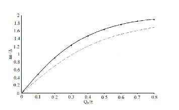
Figure 1: The dispersion $\omega/\Delta$ of the phonon-like collective mode. For filling factor $f=0.5$, lattice height $s=2.5$, and scattering length $a_{s}=-1000a_{B}$ ($a_{B}$ is the Bohr radius of hydrogen), the chemical potential $\mu=0.326E_{R}$ and the gap energy $\Delta=0.05E_{R}$ are obtained by solving the number and gap equations (4). The speed of sound in the long-wavelength limit is $8.1$ mm/s. The puncture curve represents the dispersion calculated in Ref. [SF6, ].

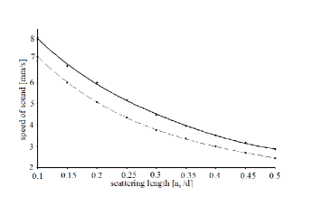
Figure 2: The speed of sound (in units mm/s) as a function of the scattering length $a_{s}/d$ ($d=515$ nm is the lattice constant). The filling factor is f=0.5, and the lattice height is $s=2.5$. The puncture curve represents the speed of sound calculated in Ref. [SF6, ].

In our numerical calculations, the sum over k is replaced by a triple integral over the first Brillouin zone: $-\pi\leq k_{x}d\leq\pi$, $-\pi\leq k_{y}d\leq\pi$ and $-\pi\leq k_{z}d\leq\pi$. After that, we applied the substitutions $x=\tan k_{x}d/4$,$y=\tan k_{y}d/4$ and $z=\tan k_{z}d/4$ to rewrite the integrals in the form of Gaussian quadrature $\int_{-1}^{1}dx\int_{-1}^{1}dyf(x,y,z)/(1+x)(1+y)(1+z)$. The corresponding integrals are numerically evaluated using $49\times 49\times 49$ $(x_{i},y_{j},z_{k})$ points: $\int_{-1}^{1}dx\int_{-1}^{1}dy\int_{-1}^{1}dzf(x,y,z)/(1+x)(1+y)(1+z)=\sum_{i=1}^{49}\sum_{j=1}^{49}\sum_{k=1}^{49}w_{i}w_{j}w_{k}f(x_{i},y_{j},z_{k})$, where $w_{i}$ is the corresponding weight. It can be checked that there is no difference between the approximation by integrals and the case when the sums over k are taken explicitly assuming 128 sites per dimension.

In Fig. 1 and Fig. 2 we present the results of our calculations of the dispersion of the phonon-like mode and the speed of sound as a function of the scattering length assuming that the filling factor and the lattice height are $f=0.5$ and $s=2.5$, respectively. The long-wavelength part of the dispersion is linear with sound velocity of about $8.1$ mm/s. For higher momenta the dispersion saturates to $2\Delta$. As it is expected, when the interaction between the atoms is increased by increasing the scattering length, the compressibility of the system increases, and therefore, the speed of sound decreases, as can be seen in Fig. 2. In both figures, there exists a difference of about 10 -15 percents between the BS approach and the response-function calculations presented in Ref. [SF6, ].

III Conclusion

In this paper, we have used the BS equations in the GRPA to obtain the dispersion of the phonon-like collective mode and the corresponding sound velocity in the long-wavelength limit in the system of equal mixture of ${}^{6}Li$ atomic Fermi gas of two hyperfine states loaded into a cubic three-dimensional optical lattice. It is shown that the previous calculations, which have been obtained by studding the poles of the density response functions, are not in accordance with our results derived by means of the BS equations in the GRPA.

References

• (1) W. Hofstetter, J. I. Cirac, P. Zoller, E. Demler, and M. D. Lukin, Phys. Rev. Lett. 89, 220407 (2002).
• (2) G. Orso and G.V. Shlyapnikov, Phys. Rev. Lett. 95, 260402 (2005).
• (3) L. P. Pitaevskii, S. Stringari, and G. Orso, Phys. Rev. A 71, 053602 (2005).
• (4) W. Hofstetter Phil. Mag., 86, 1891 (2006).
• (5) W. Yi and L.-M. Duan, Phys. Rev. A 73, 063607 (2006).
• (6) T. Koponen, J.-P. Martikainen, J. Kinnunen, and P. TΓΆrmΓ€1, Phys. Rev. A 73, 033620 (2006).
• (7) T. Koponen, J.-P. Martikainen, J. Kinnunen, LΒΏ M. Jensen, and P. TΓΆrmΓ€1, New Journal of Physics 8, 179 (2006).
• (8) M. Iskin and C. A. R. SΓ‘ de Melo, Phys. Rev. Lett. 99, 080403 (2007).
• (9) T. K. Koponen, T. Paananen, J.-P. Martikainen, and P. TΓΆrmΓ€l, Phys. Rev. Lett. 99, 120403 (2007).
• (10) T. Paananen, J. Phys. B: At. Mol. Opt. Phys. 42, 165304 (2009).
• (11) Ai-Xia Zhang and Ju-Kui Xue, Phys. Rev. A 80, 043617 (2009).
• (12) T. K. Koponen, T. Paananen, and P. TΓΆrmΓ€l, Phys. Rev. Lett. 102, 165301 (2009).
• (13) M. Iskin and C. A. R. SΓ‘ de Melo, Phys. Rev. Lett. 103, 165301 (2009).
• (14) Y. Yunomae, I. Danshita, D. Yamamoto, N Yokoshi, and S Tsuchiya, Journal of Physics: Conference Series 150, 032128 (2009).
• (15) J. K. Chin, D. E. Miller, Y. Liu, C. Stan, W. Setiawan, C. Sanner, K. Xu, and W. Ketterle, Nature (London) 443, 961 (2006).
• (16) Z. G. Koinov, Physica C 470, 144 (2010); Physica Status Solidi (B), 247 ,140 (2010).
• (17) L. Belkhir and M. Randeria, Phys. Rev. B 49, 6829 (1994).
• (18) L. Landau, Phys. Rev. 60, 356 (1941).