Multimodal transition and stochastic antiresonance in squid giant axons

Abstract

The experimental data of N. Takahashi, Y. Hanyu, T. Musha, R. Kubo, and G. Matsumoto, Physica D 43, 318 (1990), on the response of squid giant axons stimulated by periodic sequence of short current pulses is interpreted within the Hodgkin-Huxley model. The minimum of the firing rate as a function of the stimulus amplitude $I_{0}$ in the high-frequency regime is due to the multimodal transition. Below this singular point only odd multiples of the driving period remain and the system is highly sensitive to noise. The coefficient of variation has a maximum and the firing rate has a minimum as a function of the noise intensity which is an indication of the stochastic coherence antiresonance. The model calculations reproduce the frequency of occurrence of the most common modes in the vicinity of the transition. A linear relation of output frequency vs. $I_{0}$ for above the transition is also confirmed.

The Hodgkin-Huxley (HH) modelHH1952 is a prototypical resonant neuron with the main resonant frequency typically of order 40 to 60 Hz. Its output interspike intervals (ISI) can be classified in terms of integer multiples of the driving period. The multimodality is revealed when the HH neuron is stimulated by noisy inputs, such as additive noiseTiesinga2000 ; Arcas2003 , random synaptic inputsBrown1999 ; Tiesinga2000 ; Luccioli2006 or channel noiseRowat2007 . Such ISI histograms are encountered frequently in periodically forced sensory neurons. An explanation in terms of a two-state system with noise was put forward by Longtin et al.Longtin1991 . The multimodal character is manifest also in a deterministic HH model near excitation thresholdClay2003 ; Borkowski2010 and in regimes of irregular response between mode-locked statesBorkowski2010 . It was shown recently that also the parity of ISI plays a significant roleBorkowski2009 . Even (odd) modes dominate in the vicinity of even (odd) mode-locked states, respectively. The most significant manifestation of this effect is the multimodal odd-all transition between states 3:1 and 2:1Borkowski2009 , where the coefficient of variation (CV) has a maximum and the firing rate has a minimum. The notation p:q means p output spikes for every q input current pulses. Below this singularity only odd multiples of the input period exist and above it harmonics of both parities participate in the response. The transition may be crossed by varying either the stimulus amplitude or the input period. The minimum of the firing rate occurs slightly above the transition.

In earlier experiments in giant axons of squid stimulated periodically by a train of short rectangular current pulses the firing rate, defined as the ratio of the output and input frequency $f_{o}/f_{i}$, had a well pronounced minimum as a function of the interval between adjacent pulsesMatsumoto1987 or the stimulus amplitudeTakahashi1990 . Even modes were absent below the minimumTakahashi1990 . This effect occurred near the excitation threshold, between states 3:1 and 2:1. Another interesting result was the continuous relation between the firing rate and the stimulus amplitude. This set of experimental and theoretical results deserves a more detailed comparison.

The theory can be tested also by considering a periodic drive in the presence of noise. Noisy biological systemsWiesenfeld1995 ; Doiron2000 ; Stacey2001 ; Rudolph2001 ; Tiesinga2000 ; Luccioli2006 , including the HH neuron, are known to exhibit stochastic resonance (SR). This phenomenon is mainly, though not exclusively, characterized by a maximum of the signal to noise ratio as a function of the noise intensity. Another effect associated with the presence of noise is the decrease of the firing threshold and the coherence resonanceGang1993 ; Pikovsky1997 , where the minimum variability of the output signal, expressed by CV in absence of a deterministic drive, is achieved at some intermediate noise strength. Recently it was found experimentallyPaydarfar2006 ; Sim2007 theoreticallyGutkin2008 ; Gutkin2009 that small amplitude noise may decrease the firing rate or even turn it off. The nonlinear system in the vicinity of the multimodal transition is a natural candidate for finding interesting effects due to noise since the trajectories of different modes are very close in parameter space. In the following we compare experimental data to theoretical results for the deterministic case and calculate the sytem’s response to a periodic drive with additive Gaussian noise.

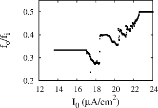
In the experiment of Takahashi et al.Takahashi1990 the squid axon was stimulated by periodic train of rectangular current steps of width $0.6\textrm{ms}$. Fig. 1 shows the experimentally obtained firing rate as a function of stimulus amplitude scaled by the minimum current threshold $I_{t}$. On the left side of the minimum only odd modes were recorded. Even modes were present at the minimum point, with the $6:1$ mode occurring more frequently than the $4:1$ component, and $2:1$ entirely absent. This is consistent with calculation resultsBorkowski2009 , where even modes disappear before reaching the multimodal transition (which is slightly below the minimum of the firing rate), with the low order modes vanishing first, beginning with mode $2:1$.

We try to reproduce this type of dependence using the HH model with the classic parameter set and rate constantsHH1952 ,

$$C\frac{dV}{dt}=-I_{Na}-I_{K}-I_{L}+I_{app},$$ (1)

where $I_{Na}$, $I_{K}$, $I_{L}$, $I_{app}$, are the sodium, potassium, leak, and external current, respectively. $C=1\mu\textrm{F/cm}^{2}$ is the membrane capacitance. The input current is a periodic set of rectangular steps of width $0.6\textrm{ms}$ and height $I_{0}$. Equations are integrated within the fourth order Runge-Kutta scheme with a time step of $0.001\textrm{ms}$. The data points are obtained from runs of 400 s, discarding the initial 4 s. The dependence of the firing rate on the stimulus amplitude is shown in Fig. 2, where $T_{i}=7\textrm{ms}$.

Figure 1: The average firing rate, $\bar{T_{o}}/T_{i}$, as a function of the stimulus amplitude $I$ from the work of Takahashi et al.Takahashi1990 . $I_{t}$ is the minimum current threshold obtained in the range $T_{i}=2.5\textrm{ms}$ to $T_{i}=6.5\textrm{ms}$. The measurements were carried out at $T_{i}=3.8\textrm{ms}$.

Figure 2: The calculated average firing rate at $T_{i}=7\textrm{ms}$ without noise.

The similarity to experiment is striking. Although the calculated minimum occurs at almost twice the experimental $T_{i}$, the other time scales such as the refractory period and the time span of the bifurcation diagram differ by a similar factor. The entire dynamics of the axon from the study of Takahashi et al. is significantly faster than that of Hodgkin and Huxley. This difference of time scales is not unusual. Long time ago BestBest1979 noted that the axon used by Hodgkin and Huxley was of poor quality and in later studies significantly higher conductivities were obtained. Paydarfar et al.Paydarfar2006 in their recent study recorded firing periods in the range between 7 and 16 ms. The overall dynamics of Figs. 1 and 2 agrees very well, including the location and depth of the local minima. We verified that the form of Fig. 2 was unchanged for pulse widths between 0 and $1\textrm{ms}$ after dividing the current amplitude by $\int_{0}^{T_{i}}I(t)dt$.

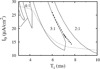
Fig. 3 shows the response diagram in the high-frequency limit. The dotted line separates the monostable firing solution from the silent state and bistable areas where the limit cycle coexists with a fixed point solution. Boundaries of bistability were determined using a continuation method starting from a region with a single solution.

Figure 3: The bifurcation diagram in the $T_{i}$-$I_{0}$ plane, showing the main mode-locked states in the model without noise. The unmarked intrusion in the upper left corner is the 5:1 state. The bottom part of the figure is occupied by the silent state. In the firing part of the diagram there are two solutions below the dotted line. Here the limit cycle coexists with the fixed point. Full squares show the location of the minima of the firing rate. The borders of states below $T_{i}=4.5\textrm{ms}$ are shown in an approximate form. The detailed picture is less regular and somewhat more complex.

Table 1: Frequency of occurrence of the six lowest modes at the minimum of the firing rate. The upper row is based on Fig. 13e from the experimental data of Takahashi et al.Takahashi1990 . The bottom row is the result of calculations, assuming $T_{i}=7\textrm{ms}$ and $I_{0}=18\mu\textrm{A/cm}^{2}$ (see Fig. 4).

mode
2	3	4	5	6	7
0	0.66	0.04	0.12	0.09	0.04
0.002	0.74	0.07	0.11	0.04	0.02

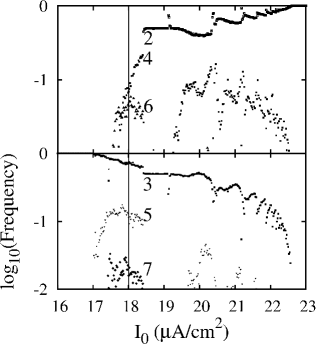
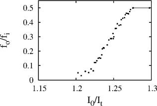
The experimental local maximum on the plateau $f_{o}/f_{i}=0.4$ is due to the state 10100, where modes 2:1 and 3:1 alternate. The other local maximum at $f_{o}/f_{i}=0.429$ with tendency to lock into the $\textrm{(10)}^{2}100$ was also reproduced. Fig. 4 shows the relative frequency of participation of the most common modes on a logarithmic scale. Higher-order modes appear more frequently near the minimum of the firing rate. Experimental and calculated ISI histograms are compared in Table 1. The overall agreement is quite remarkable. Also the calculated evolution of individual modes as a function of $I_{0}$ is close to measured values. In experiment the probability of appearance of mode 4:1 between $I_{0}/I_{t}=1.2$ and 1.3 remains in the range $0.06$ to $0.08$, which agrees well with Fig. 4 for $I_{0}$ between $18\mu\textrm{A/cm}^{2}$ and $22\mu\textrm{A/cm}^{2}$. The published experimental runsTakahashi1990 contain 80 to 100 output spikes for selected data points. On the basis of this data set we can conclude that the frequency of participation of the low order modes is approximately reproduced in simulations. Above the multimodal transition the experimental firing rate near the threshold rises linearly with the stimulus amplitude, see Fig. 5. The dependence of $f_{o}/f_{i}$ vs. of $I_{0}$ is well reproduced in Fig. 6, except in the vicinity of the 2:1 plateau, where an addition of a small amount of noise would improve the fit.

Figure 4: The relative frequency of occurrence of low-order even and odd modes for the parameter set of Fig. 2 The vertical line marks the position of the minimum of the firing rate.

Figure 5: The linear relation of the firing rate vs. the stimulus amplitude above the multimodal transition point at $T_{i}=4\textrm{ms}$. These are experimental results of Takahashi et al.Takahashi1990 .

Figure 6: Calculated average firing rate vs. stimulus amplitude above the multimodal transition for three values of $T_{i}$. The current pulse width is $0.6\textrm{ms}$.

We now consider the model with a Gaussian white noise:

$$C\frac{dV}{dt}=-I_{Na}-I_{K}-I_{L}+I_{app}+C\xi(t),$$ (2)

where $<\xi_{i}(t)>=0$, $<\xi(t)\xi(t^{\prime})>=2D\delta(t-t^{\prime})$, and $D$ is expressed in $\textrm{mV}^{2}/\textrm{ms}$. The HH equations are integrated using the second-order stochastic Runge-Kutta algorithmHoneycutt1992a . The simulations are carried out with the time step of $0.01\textrm{ms}$ and are run for 400 s, discarding the initial 40 s.

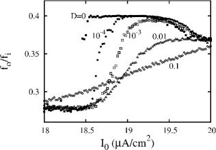
There is a tendency to assume that biological systems, including neurons, should always be treated as noisy systems. While the neuron is sensitive to noise it is not obvious that single neuron dynamics should always include stochastic terms. Fig. 7 shows the quick disappearance of the $f_{o}/f_{i}=0.4$ plateau in Fig. 2 with increasing noise. Comparing with the experimental data in Fig. 1 we conclude that calculations reproduce experimental data only for $D<10^{-4}$.

Figure 7: Sensitivity of the $f_{o}/f_{i}=0.4$ plateau from Fig. 2 to noise.

Certainly more experiments are needed to understand the role of noise in neurons.

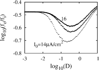
Fig. 8 presents the firing rate as a function of $D$ for three parameter sets from the $3:1$ plateau of Fig. 2. For small noise $f_{o}/f_{i}$ drops quickly below $1/3$ over an entire plateau, with the biggest drop near the edges. This behavior should be contrasted with the resonant regime where the central part of each plateau maintains phase locking over much larger range of noise intensities and $D\sim 1$ is needed to lower the firing rate of an entire plateau below the $D=0$ valueBorkowski2010 . Another difference is the direction of frequency changes at the plateau edges. In the resonant state the frequency below (above) the plateau midpoint is lowered (increased), respectivelyBorkowski2010 . In the antiresonant limit the entire plateau is unstable to even a small noise which slows down the system considerably.

Figure 8: The firing rate vs. the noise intensity. The middle curve was obtained for $I_{0}=15\mu\textrm{A/cm}^{2}$. Here $T_{i}=7\textrm{ms}$. At $D=0$ all three curves start in the 3:1 mode.

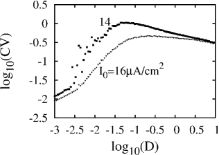
CV as a function of $D$ has a maximum for the same parameter set, see Fig. 9. The increased variability is associated with increased participation of higher-order modes and may be called a stochastic coherence antiresonance. A maximum of CV was found earlier in a leaky integrate-and-fire model with an absolute refractory period for suprathreshold base currentLindner2002 . A small local maximum of CV at intermediate noise level was also found by Luccioli et al.Luccioli2006 in a HH model driven by a dc current in a bistable regime, where the neuron was stimulated by a large number of stochastic inhibitory and excitatory postsynaptic potentials. It was pointed out that the stochastic antiresonance may exist in regions of bistabilityGutkin2009 , when the stable limit cycle coexists with other attractors. This typically occurs in the vicinity of a bifurcation when the value of the bifurcation parameter slightly exceeds the critical value. In the HH model near the multimodal transition there are many competing limit cycles. Noise enhances trajectory switching and may even stop the firing entirely. A decrease of the firing rate and an increase of incoherence may occur along much of the excitation threshold, where the deterministic system is bistable or responds irregularlyBorkowski2010 .

Figure 9: The maximum of the coefficient of variation as a function of the noise intensity is a property of the stochastic coherence antiresonance. The maximum of CV and the minimum of the firing rate occur at different noise levels. The irregularity of the $I_{0}=14\mu\textrm{A/cm}^{2}$ curve is a consequence of proximity to the excitation threshold.

In conclusion, numerical solutions of the deterministic HH equations show that the minimum of the firing rate observed by Takahashi et al.Takahashi1990 is due to the multimodal transitionBorkowski2009 . The statistics of the experimental spike trains confirm that below the transition only odd modes remain. Even modes are present at the minimum of $f_{o}/f_{i}$, in agreement with theoretical calculationsBorkowski2009 . The calculated frequencies of occurrence of the most common modes are close to experimental values. Also the location of the minimum of $f_{o}/f_{i}$ in the vicinity of the 3:1 state is consistent with the simulations. The linear rise of the output frequency as a function of the stimulus strength above the multimodal transition was also confirmed. The excitation threshold in the antiresonant limit is higher by about a factor of two compared to the resonant regime. The rise of threshold for frequencies of current pulses exceeding the resonant frequency was observed experimentally by Kaplan et al.Kaplan1996 . Further support for the significance of the parity of the modes comes from the experiment of Paydarfar et al.Paydarfar2006 , who found that the quiescent periods between highly regular bursts were always equal to even multiples of the resonant period. An ISI histogram with odd modes was obtained by Racicot and LongtinRacicot1997 in a chaotically forced FitzHugh-Nagumo (FHN) model. FHN equations are often used as a substitute for the full HH model. It would therefore be useful to investigate whether the main features of the odd-all ISI transition are reproduced in the FHN model with a deterministic and stochastic drive.

Perturbing the system with noise changes significantly the $f$ vs. $I_{0}$ dependence. The local minima of this curve disappear already for $D\simeq 10^{-3}$. In the regime below the multimodal transition the 3:1 plateau disappears rapidly for very small noise. The firing rate has a minimum and CV has a maximum as a function of the noise intensity. These predictions are expected to be valid for short stimuli of different shapes and can be tested experimentally. The multimodal transition and the accompanying stochastic antiresonance are important both for the understanding of excitable systems and for potential neurological applications. Spike annihilation by deterministic signalsGuttmanLewisRinzel1980 is studied in the context of deep brain stimulationTass2002 ; Calitoiu2007 , a therapeutic technique, in which synchronicity of certain parts of the brain is reduced by brief current pulses.

References

- (1) A. L. Hodgkin and A. F. Huxley, J. Physiol. (London) 117, 500 (1952).
- (2) P. H. E. Tiesinga, J. V. José, and T. J. Sejnowski, Phys. Rev. E 62, 8413 (2000).
- (3) B. Agüera y Arcas, A. L. Fairhall, W. Bialek, Neural Comput. 15, 1715 (2003).
- (4) D. Brown, J. Feng, and S. Feerick, Phys. Rev. Lett. 82, 4731 (1999).
- (5) S. Luccioli, T. Kreuz, and A. Torcini, Phys. Rev. E 73, 041902 (2006).
- (6) P. Rowat, Neural Comput. 19, 1215 (2007).
- (7) A. Longtin, A. Bulsara, and F. Moss, Phys. Rev. Lett. 67, 656 (1991).
- (8) J. R. Clay, J. Comput. Neurosci. 15, 43 (2003).
- (9) L. S. Borkowski, Nonlinear dynamics of Hodgkin-Huxley neurons (Adam Mickiewicz University Press, 2010).
- (10) L. S. Borkowski, Phys. Rev. E 80, 051914 (2009).
- (11) G. Matsumoto, K. Aihara, Y. Hanyu, N. Takahashi, S. Yoshizawa, and J. Nagumo, Phys. Lett. A 123, 162 (1987).
- (12) N. Takahashi, Y. Hanyu, T. Musha, R. Kubo, and G. Matsumoto, Physica D 43, 318 (1990).
- (13) K. Wiesenfeld and F. Moss, Nature 373, 33 (1995).
- (14) B. Doiron, A. Longtin, N. Berman, and L. Maler, Neural Comput. 13, 227 (2000).
- (15) W. C. Stacey and D. M. Durand, J. Neurophysiol. 86, 1104 (2001).
- (16) M. Rudolph and A. Destexhe, J. Comput. Neurosci. 11, 19 (2001).
- (17) Hu Gang, T. Ditzinger, C. Z. Ning, and H. Haken, Phys. Rev. Lett. 71, 807 (1993).
- (18) A. S. Pikovsky and J. Kurths, Phys. Rev. Lett. 78, 775 (1997).
- (19) D. Paydarfar, D. B. Forger, and J. R. Clay, J. Neurophysiol. 96, 3338 (2006).
- (20) C. K. Sim and D. B. Forger, J. Biol. Rhythms 22, 445 (2007).
- (21) B. S. Gutkin, J. Jost, and H. C. Tuckwell, Europhys. Lett. 81, 20005 (2008).
- (22) B. S. Gutkin, J. Jost, and H. C. Tuckwell, Naturwissenschaften 96, 1091 (2009).
- (23) E. N. Best, Biophys. J. 27, 87 (1979).
- (24) R. L. Honeycutt, Phys. Rev. A 45, 600 (1992).
- (25) B. Lindner, L. Schimansky-Geier, and A. Longtin, Phys. Rev. E 66, 031916 (2002).
- (26) D. T. Kaplan, J. R. Clay, T. Manning, L. Glass, M. R. Guevara, and A. Shrier, Phys. Rev. Lett. 76, 4074 (1996).
- (27) D. M. Racicot and A. Longtin, Physica D 104, 184 (1997).
- (28) R. Guttman, S. Lewis, and J. Rinzel, J. Physiol. 305, 377 (1980).
- (29) P. A. Tass, Phys. Rev. E 66, 036226 (2002).
- (30) D. Calitoiu, B. J. Oommen, and D. Nussbaum, Biol. Cybern. 98, 239 (2007).