Spectral Variability of Romano’s Star

Abstract

We combine archival spectral observations of the LBV star V532 (Romano’s star) together with the existing photometric data in the B band. Spectroscopic data cover 15 years of observations (from 1992 to 2007). We show that the object in maximum of brightness behaves as an emission line supergiant while in minimum V532 moves along the sequence of late WN stars. In this sence, the object behaves similarly to the well-known Luminous Blue Variable (LBV) stars AG Car and R127, but is somewhat hotter in the minima. We identify about 100 spectral lines in the $3700\div 7300$$\rm\AA$ wavelength range. For today, our spectroscopy is the most comprehensive for this object. The velocity of the wind is derived using HeI triplet lines ($360\pm 30{\rm km\leavevmode\nobreak\ s^{-1}}$). Physical parameters of the nebula around V532 are estimated.

stars: individual: Romano’s star (M33) galaxies: individual: M33 stars: supergiants stars: Wolf-Rayet

0.1 Introduction

Luminous Blue Variables (LBVs) are a class of rare astrophysical objects introduced by Conti (1984) and remain a subject of intense interest. LBVs are broadly accepted as very massive and energetic stars emitting close to the Eddington limit, evolving from Of toward Wolf-Rayet stars. However, contemporary evolutionary models do not answer the question about the exact relations between LBV, nitrogen-rich Wolf-Rayet (WN) and hydrogen-rich WN (WNH) stars. Numerical simulations show that the objects may pass the LBV evolutionary stage either before or after the WNH stage (Smith & Conti 2008). Currently, only 35 LBV and LBV candidates are known in our Galaxy (Clark et al. 2005). Studying LBVs in nearby galaxies is very important for understanding stellar evolution and the evolution of the interstellar medium perturbed and contaminated by massive stars at various evolutionary stages.

The object V532 ($\alpha=01^{h}35^{m}09.^{s}71$, $\delta=+30^{o}41^{\prime}\!\!\!\,\leavevmode\nobreak\ 57^{\prime\prime}\!\!\!.\,1$) is located in the outer spiral arm of the M33 galaxy. Giuliano Romano was the first to recover its light curve (Romano 1978) and to find irregular magnitude variations between 16${}^{\rm m}\!\!\!.\,7$ and 18${}^{\rm m}\!\!\!.\,1$. Romano classified V532 as a variable of the Hubble-Sandage type by the shape of the light curve and its colour index. Humphreys & Davidson (1994) on the basis of its light variations classified the star as an LBV candidate. Two maxima of brightness were detected during the last half of the century (Kurtev et al. 2001). The first was observed around 1970 and the second in the early 1990s (Kurtev et al. 2001). Long-term variability has an amplitude of about 1${}^{\rm m}\!\!\!\,\,$ and seems to be superimposed on an even stronger downward trend. Short-timescale variability with amplitude $\sim$0${}^{\rm m}\!\!\!.\,$5 was discovered in addition to the longer-timescale variability (Kurtev et al. 2001; Sholukhova et al. 2002). Such photometric behavior is typical for an LBV star.

First optical spectrum was obtained by T. Szeifert (Szeifert 1996) at the 3.5 m Calar Alto telescope in 1992. In this spectrum, “few metal lines are visible, although a late B spectral type is most likely (faint HeI)”. This spectrum, obtained with the TWIN spectrograph of the Calar Alto telescope, is unique in being obtained in a profound flare state. It is drastically different from the hot spectra observed in the minima of brightness (see below).

Second spectrum was obtained by O. Sholukhova at the 6m telescope of the Special Astrophysical Observatory (SAO) of Russian Academy of Sciences (RAS) in 1994 (Sholukhova et al. 1997). Another spectrum was obtained at SAO with the Multi-Pupil Fiber Spectrograph (MPFS) in September 1998. This spectrum was classified as WN10–WN11 Fabrika et al. (2005). Polcaro et al. (2003) estimated the bolometric absolute magnitude of the object as $M_{bol}\simeq-10^{\rm m}\!\!\!.\,4$, using bolometric correction “of at least -3 mag” and distance modulus $m-M=24^{\rm m}\!\!\!.\,8$. They classify V532 as an LBV because the object fulfills all the criteria of Humphreys & Davidson (1994). Using five spectra carried out in 2003 $\div$ 2006, Viotti et al. (2006, 2007) find anti-correlation between equivalent widths of the Wolf-Rayet blue bump at $4630\div 4686$$\rm\AA$ and visual luminosity.

Comparing the spectra published by Szeifert (1996), Fabrika et al. (2005) and Viotti et al. (2007), we find that the object changes its spectral properties significantly.

Here we combine the spectral observations (both new and already published) with the light curve of the object to trace the spectral variability of the star. We describe the data and data reduction process in the next section. Results are presented in section 0.3 and discussed in section 0.4. In section 0.5, we present the conclusions.

Table 1: Observational log for MPFS data. S/N is signal-to-noise ratio per resolution element.

Date	Exposure	Seeing, ${}^{\prime\prime}\!\!\!$	S/N	Spectral	Spectral
	time, s			standard star	range, $\rm\AA$
05. 10. 2002	900	3.8	16	BD25d4655	4250-6700
13. 11. 2004	4200	1.5	20	HZ44	4000-7000
17. 01. 2005	3600	1.5	18	G248	4000-7000

0.2 Observations and Data Reduction

In this work, we use archival data from the 6m SAO telescope (available via ASPID database, http://alcor.sao.ru/db/aspid/) and the SUBARU telescope, which is operated by the National Astronomical Observatory of Japan. The 6m telescope data were obtained with the Multi Pupil Fiber Spectrograph (MPFS) (Afanasiev et al. 2001) and with the SCORPIO multi-mode focal reducer in the long-slit mode (Afanasiev & Moiseev 2005). The data from SUBARU were obtained with the Faint Object Camera (FOCAS) (Kashikawa et al. 2002) in the Cassegrain focus. Uncertainties are everywhere dominated by statistical Poissonian noise (readout noise and round-off errors are significantly smaller).

0.2.1 MPFS Data

MPFS obtains simultaneously the spectra from 240 ($16\times 15$) or 256 ($16\times 16$) spatial sampling elements arranged in the form of a rectangular array of square lenses. In 2002 and 2004-2005, the data were obtained in the 240-element and 256-element configurations, respectively. Spatial sampling of 1${}^{\prime\prime}\!\!\!\,\,\times$1${}^{\prime\prime}\!\!\!\,\,$ was used. Light from individual sampling elements is collected by microlenses and transmitted by means of optical fibers reorganized in the form of a pseudo-slit toward the spectral camera. Grating # 4 (600 $\rm\AA$ $\rm pix^{-1}$) providing spectral resolution of about 6 $\rm\AA$ was used for all the observations. Detectors CCD TK 1024 ($1024\times 1024$ pixels) and EEV42-40 ($2048\times 2048$ pixels) were used in 2002 and 2004-2005, correspondingly. Sky background spectrum at the distance of 4${}^{\prime}\!\!\!\,\,$ away from the object is taken simultaneously with the object by 17 (for 16$\times$16 field size) or 16 (for 16$\times$15 configuration) additional fibres. We summarize the relevant information on the MPFS data in table 1.

Data reduction system was written in IDL environment and makes use of procedures written by V. Afanasiev, A. Moiseev and P. Abolmasov. Reduction process consists of the standard steps for panoramic data reduction (see for example Sánchez (2006)): bias subtraction, flat-fielding, removal of cosmic-ray hits, extraction of the individual spectra from the frames and their wavelength calibration using a spectrum of an He-Ne-Ar lamp. At every wavelength, we calculate the median sky level using the offset fibres and subtract from the spectra of the field. Spectra of spectrophotometric standard stars were used for absolute flux calibration.

Three emission-line spectra obtained with MPFS in 2002-2005 were used. We estimate signal-to-noise ratio in continuum as 10$\div$30 per resolution element (see table 1 for details). Integral spectra were extracted in an annular aperture $2^{\prime\prime}\!\!\!\,\,$ in radius. Up to the instrumental resolution, the object point-like. Note that, unlike long-slit spectrographs, MPFS is free from slit losses at absolute flux calibration is much more reliable.

0.2.2 SCORPIO Data

Observational data from SCORPIO are summarized in table 2. All the spectra were reduced using ScoRe package for long-slit data reduction, written in IDL (available at http://narod.ru/disk/5238009000/Score_v1.2.tar.html). CCD frames were de-biased, cosmic particle hits were removed from all types of exposures except bias. Save for the single 10 minute long exposure obtained in February 2005, several object exposures are present for every day that simplifies the removal of cosmic hits. Then we divide object and spectral standard exposures over normalized mean flat-field frame. After wavelength calibration using He-Ar-Ne lamps and night sky OI ($\lambda 5577$ or $\lambda 6300$ depending on grism) emission lines, the CCD data were flux-calibrated using standard stars from Oke (1990) spectrophotometric standard list (see table 2). Spectra were extracted by fitting the profiles of slices across dispersion with Gaussian function.

In total, eight spectra were obtained with SCORPIO in 2005-2008 (dates of observations are shown by upward arrows in figure 1). Spectral resolution is 10 $\rm\AA$(for VPHG550G grism) and 5 $\rm\AA$(for VPHG1200G and VPHG1200R grisms), signal-to-noise ratios in continuum vary from about 10 to about 50 for larger total exposures.

Table 2: Observational log for the SCORPIO data. $\alpha$ is seeing, PA is position angle, S/N is signal-to-noise ratio.

-0.5cm-0.5cm 8 Date Exposure Grism Spectral $\delta\lambda,$ S/N $\alpha,\leavevmode\nobreak\ ^{\prime\prime}\!\!\!$ Spectral PA,^o time, s range, $\rm\AA$  $\rm\AA$ standard star 6. 02. 2005 600 8 1.7 G248 -136 30. 08. 2005 1200 VPHG550G 3500-7200 10 30 1.9 G191-B2B 210 8. 11. 2005 3300 45 1.9 BD25d4655 145 3. 08. 2006 1500 20 2 GD248 200 10. 08. 2007 1800 VPHG1200G 4000-5700 5 24 2 BD33d2642 252 5. 10. 2007 2700 40 1.1 BD25d4655 -141 8. 01. 2008 1800 VPHG1200R 5700-7500 5 20 2.1 BD25d4655 48 10. 01. 2008 1800 VPHG1200G 4000-5700 5 20 1.4 BD25d4655 18

Figure 1: B-band light curve of V532. Arrows indicate when spectroscopic observations were made. Data from (Viotti et al. 2007) are shown by diamonds.

0.2.3 Data from SUBARU

One exposure 1200s in length was obtained with the SUBARU telescope in October 2007. VPHG450 grism was used providing the spectral range of 3750-5250 $\rm\AA$. Slit width of 0${}^{\prime\prime}\!\!\!.\,5$ implies spectral resolution of about 1.7 $\rm\AA$ (for today, it is the best resolution achieved for this object) in the extracted spectrum. Data were reduced using IDL-based software. The CCD frames were bias-subtracted and flat-fielded. We used the Th-Ar arc spectrum for wavelength calibration. Star BD40d4032 from SUBARU spectrophotometric standard list was used to calibrate the stellar spectra. We extract the spectrum in the same way we did it for SCORPIO (see above section 0.2.2)

If we degrade the spectral resolution to 5$\rm\AA$, the spectrum becomes practically identical to the spectrum obtained with SCORPIO on the same date. Though the spectral shapes are similar, the spectra differ in normalization (about a factor of three) connected to slit losses.

0.2.4 Photometric Data

The light curve (see figure 1) was provided by Vitalij Goranskij and consists of the CCD data obtained by Goranskij and Zharova with the 1m SAO telescope and two instruments of the Crimean laboratory of the Sternberg Astronomical Institute (SAI) and photographic plates from the SAI collection. CCD data were reduced with MaxIm DL software (http://www.cyanogen.com/maxim_main.php). The joint light curve will be published by Zharova et al. (2010) in a separate paper, all the details of the data reduction process will be given there. Photographic B-band magnitudes were identified with the B-band magnitudes obtained by CCD observations. CCD data uncertainties are of the order $0^{\rm m}\!\!\!.\,05$, plate data have larger errors depending on the source brightness, usually of the order $0.1-0.2^{\rm m}\!\!\!\,\,$.

The joint curve contains the data of Viotti et al. (2007) but complements it with a much larger photometric material and primarily allows to trace the recent evolution of the object.

0.3 Results

0.3.1 Spectral Evolution

6 -1cm1cm 8 $\lambda$, $\rm\AA$ Ion EW EW $\lambda$, $\rm\AA$ Ion EW EW emission, absorption, emission absorption $\rm\AA$ $\rm\AA$ $\rm\AA$ $\rm\AA$ 3770.60 H11+HeII 4613.90 NII 3797.90 H10+HeII 4621.40 NII 3819.76 HeI 4630.54 NII 3835.39 H9+HeII 4634.00 NIII $6.2\pm 1.0$ 3871.82 HeI 4640.64 NIII $7.4\pm 0.5$ 3889.05 H8+HeI $11\pm 1$ $3.7\pm 1.3$ 4643.09 NII 3964.73 HeI 4650.16 C III $5.0\pm 0.5$ 3970.08 H$\epsilon$+HeII 4658.10 [FeIII] $2.5\pm 1.0$ 3994.99 NII 4685.81 HeII $15.2\pm 0.2$ 4009.00 HeI 4701.50 [FeIII] $2.9\pm 1.0$ 4025.60 HeI+HeII 2.5$\pm$0.5 1.2$\pm$0.2 4713.26 HeI $1.6\pm 0.2$ 4088.90 SiIV 4861.33 H$\beta$ $22.5\pm 1.5$ 4097.31 N III 4921.93 HeI 4.3$\pm$0.2 4101.74 H$\delta$+HeII 7.6$\pm$1.0 4958.91 [O III] 1.3$\pm$0.2 4103.40 NIII 5006.84 [O III] 3.9$\pm$0.6 4116.10 SiIV 5015.67 HeI 2.6$\pm$0.3 4120.99 HeI 5411.50 HeII 6.2$\pm$0.2 4143.76 HeI 5666.60 NII 4199.80 HeII 5676.02 NII 4236.93 NII 5679.56 NII 4241.79 NII 5686.21 NII 4241.79 NII 5710.76 NII 4340.47 H$\gamma$+HeII 8.0$\pm$0.3 5875.79 HeI 25.5$\pm$0.7 4387.93 HeI 1.4$\pm$1.0 6548.00 [N II] 4471.69 HeI 5.0$\pm$0.3 1.7$\pm$0.2 6562.82 H$\alpha$+HeII 107$\pm$3 4481.13 MgII 6583.00 [N II] 4510.90 NIII 6678.15 HeI 18 $\pm$3 4514.90 NIII 6683.20 HeII 4518.20 NIII 7065.44 HeI 18 $\pm$3 4523.60 NIII 7135.73 ArIII $3.2\pm 0.3$ 4530.80 NIII 7281.35 HeI 4534.60 NIII 4541.60 HeII 4547.30 NIII 4601.50 NII 4607.20 NII

Table 3: List of emission lines detected in the FOCAS and SCORPIO (January 2008) spectra of V532. For higher signal-to-noise ratios, equivalent widths (EW) are given. For lines with P Cyg profiles, we give both emission and absorption component EWs.

The first optical spectrum of V532 was obtained during the rise of brightness, when the object was 16${}^{\rm m}\!\!\!.\,$4 in the V band. This spectrum covers two spectral ranges $\lambda\lambda 4400-5000$ and $\lambda\lambda 5800-6750$, as it was obtained with the two-channel TWIN spectrograph (a comprehensive description is present at http://www.caha.es/CAHA/Instruments/TWIN/HTML/twin.html). In this spectrum, two strong lines are present, $H\alpha$ (shown in figure 2) and $H\beta$, having complex profiles consisting of a narrow line with P Cyg profile and broad wings. FWHM (Full Width at Half Maximum intensity) of the wings is $\sim 15\rm\AA$ for H$\beta$ and $\sim 20\rm\AA$ for H$\alpha$. Such wings were first found for LBVs in the spectrum of P Cygni by Bernat & Lambert (1978). These wings are explained by scattering of line photons by free electrons in the stellar wind. Similar line profiles were observed for the LBV stars R127 and AG Car during the initial rise to maxima (Stahl et al. 1983, 2001).

Emission lines of HeI$\lambda 5876$ and SiII$\lambda 5957.612,5978.970,6347.091,6371.359$ are also present in the red spectrum. Szeifert (1996) mentions these SiII lines as “weak metal emissions”.

Figure 2: H$\alpha$ line profile in the Calar Alto spectrum obtained in 1992. The spectrum is normalized by the local continuum level.

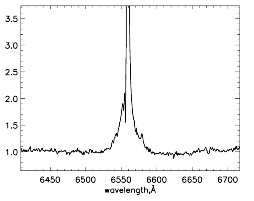
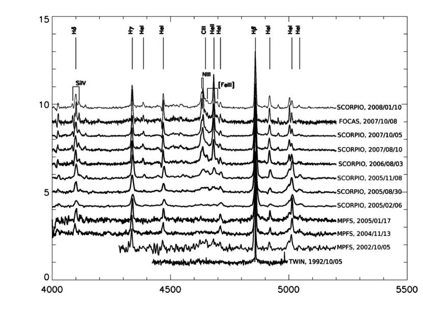
Figure 3 shows all the spectra of V532 in the blue range (4000-5500$\rm\AA$) analysed in this article, obtained at different spectral resolutions. All the spectra are normalised to continuum level in a uniform way. In order to get a reasonable normalisation for our spectra, we chose several wavelength intervals practically free from Wolf-Rayet emissions (4250$\div$4270, 5100$\div$5200, 5520$\div$5620, 5750$\div$5800 and 6950$\div$6970$\rm\AA$) and reconstructed the continuum using a second-order polynomial. Below, for spectral classification we use characteristic equivalent width ratios, that makes our results practically independent of spectral resolution.

The spectral appearance of the spectra of V532 obtained in 2002-2008 resembles that of late WN stars. It allows to apply a classification scheme used for WN stars, bearing in mind that abundances of individual elements may differ, but physical conditions are similar. All the spectra obtained between 2002 and 2008 were classified using the classification of Smith, Crowther & Prinja (1994) for WN6-11 stars based primarily on relative strengths of NV $\lambda\lambda 4604-20$, NIV $\lambda 4058$, NIII $\lambda\lambda 4634-41$ and NII $\lambda 3995$ emission lines. The method has low dependence on elemental abundances, though only helium and nitrogen lines (preferably, ratios of the lines of one element) are used. The results of spectral classification are given in table 4.

6

Table 4: Spectral classes identified via the scheme of Smith, Crowther and Prinja (1994)

B, mag	Spectral	Date			B, mag	Spectral	Date
	subtype					subtype
17.5	WN10.5	2002/10/05			17.6	WN9	2005/11/08
16.9	WN11	2004/11/13			18.3	WN8	2006/08/03
17.1	WN11	2005/01/17			18.4	WN8	2007/08/10
17.15	WN11	2005/02/06			18.5	WN8	2007/10/05-08
17.3	WN10	2005/08/30				WN8	2008/01/08-10

Figure 3: Optical spectrum evolution in the blue spectral range (4000$\div$5200$\rm\AA$). Spectra are normalized by the local continuum level and vertically shifted for clarity.

Light curve exhibits a local maximum in 2004 and early 2005. In the spectra obtained in this period, one may observe strong emission lines of hydrogen and neutral helium. The spectral appearance of V532 shows strong similarities with a spectrum of a WN11 star. HeI $\lambda 4713$ line is stronger than the NII blend, and HeII$\lambda 4686$ is absent. In the spectrum obtained in 2002, the NII $\lambda$3995 line is outside the spectral range, therefore we carry out classification comparing NIII $\lambda\lambda 4634-41$ and NII $\lambda\lambda 4601-43$ blends having similar intensity to the NII $\lambda$3995 emission. NIII $\lambda\lambda 4634-41$ lines appear, but are weaker than NII $\lambda\lambda 4601-43$. HeII$\lambda 4686$ line is approximately as bright as the NII $\lambda\lambda 4634-41$ emission, hence we classify the object as WN10.5.

Starting from the middle of 2005, Romano’s star weakens in the optical range, its visible magnitude falls from 17 to 18${}^{\rm m}\!\!\!.\,$8. During this period its spectrum evolves from WN10 (August 2005) through WN9 (November 2005) to WN8 (August 2007) by three spectral sub-classes. In October 2007, HeII $\lambda$4686 line is stronger than NIII $\lambda\lambda 4634-41$. However, NIV lines do not appear in the spectrum. We also classify the spectrum as WN8.

Figure 4: Left panel: V532 location on equivalent width diagram of ${\rm HeI}\lambda 5876$ versus ${\rm HeII}\lambda 4686$ for different dates of observation. The points are connected with dotted lines in chronological order. Right panel: V532 location in October 2007 (FOCAS data) on equivalent width versus FWHM diagram for the ${\rm HeII}\lambda 4686$ line. In both graphs, known Galactic (open symbols) and LMC (filled) WN stars are shown for comparison: WN8 by circles, WN9 by squares, and WN10 by triangles. Data on these objects were taken from Smith et al. (1995).

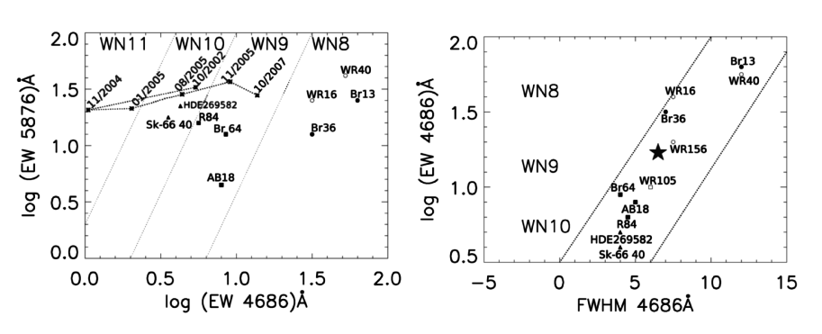
V532 evolution on the equivalent width diagram of HeI $\lambda 5876$ versus HeII $\lambda 4686$ is shown in the left panel of figure 4. Locations of well-proven Galactic and Large Magellanic Cloud (LMC) Wolf-Rayet stars R84 (WN9), Sk-60 40 (WN10), LBV HDE 269582 (WN10) and some other objects are shown for comparison with our object. The figure shows that in the period between 2002 and 2005, when the star brightened by about one magnitude, its spectrum changed from WN9.5 to WN11. Since 2005, the spectrum changes smoothly according to the sequence established by Smith, Shara & Moffat (1996).

We used a quantitative chemistry-independent criterion based on the FWHM of the HeII $\lambda 4686$ line for alternative spectral classification. In Fig.4, we show the location of V532 on the diagram of the equivalent width of HeII $\lambda 4686$ versus FWHM of this line. We have measured equivalent width and FWHM of the HeII line in the FOCAS spectrum. For this, we approximate Wolf-Rayet blue bump by 7 Gaussians. The position of V532 is fully consistent with its Galactic and LMC WN9 analogues. Spectral class defined from the diagram is consistent with that determined from the relative strengths of NII, NIII and HeI with accuracy about one subclass.

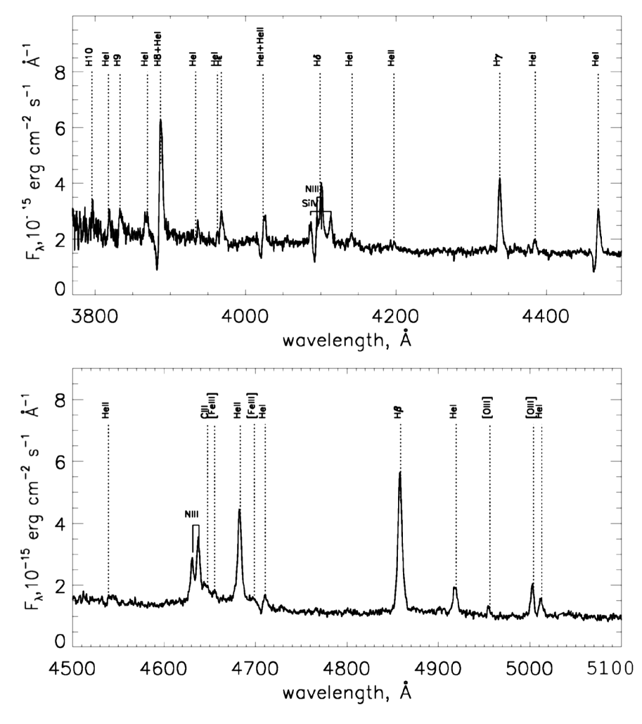
Table 3 shows the lines detected in the spectra obtained with FOCAS (October 2007) and with SCORPIO (January 2008, with grisms 1200G and 1200R). Three spectra are used in order to cover the maximal wavelength range at maximal possible spectral resolution. The spectrum of V532 does not change noticeably from October 2007 to January 2008. Equivalent widths of the principal lines (absorptions, emissions and P Cyg) are given with errors of approximation. Uncertainties due to the choice of the continuum level are smaller than the errors of approximation. Lines with P Cygni profiles were resolved by fitting with the models described in the next subsection.

0.3.2 Line Profiles and Terminal Wind Velocity

In figure 5 we show the FOCAS spectrum in the optical blue range $3800-5100\rm\AA$. The Wolf-Rayet blue bump (consisting primarily of NIII$\lambda\lambda 4634,4640$, CIII$\lambda 4650$, HeII$\lambda 4686$ and HeI$\lambda 4713$) is clearly seen in this spectrum. We suppose that the lines near 4658 and 4701 $\rm\AA$ are nebular lines of [FeIII]. They can not belong to CIV since CIV $\lambda\lambda 5812,5801$ lines are not present in the SCORPIO spectrum obtained simultaneously in October 2007.

Figure 5: Optical spectrum of V532 obtained with FOCAS in the range 3800-5100$\rm\AA$$\rm\AA$.

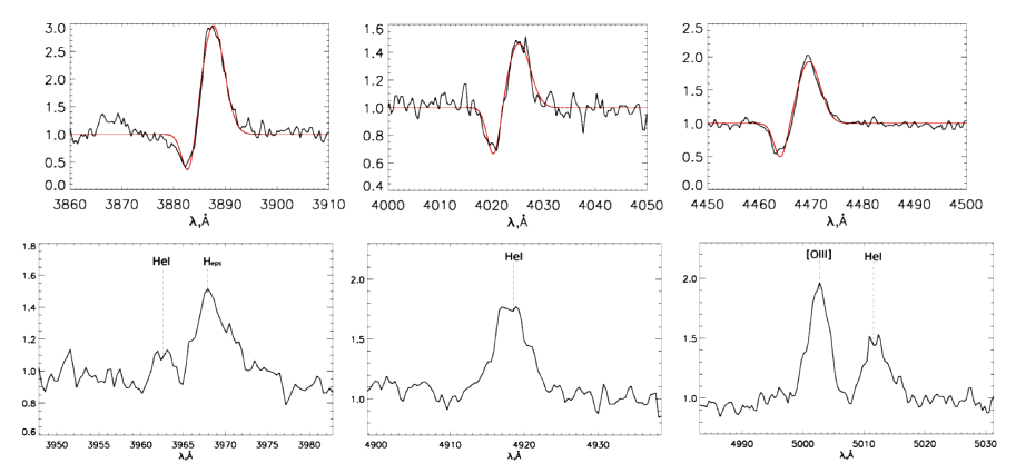
Analyzing the FOCAS spectrum of V532, we found that triplet and singlet lines of HeI have different profiles (see figure 6). Triplet lines of HeI ($\lambda 3889,4025,4471$) show strong P Cyg profiles, while singlet lines ($\lambda 3965,4922,5016$) have flat-topped profiles. Widths of these lines correspond to velocity span of about $100\leavevmode\nobreak\ \rm km\leavevmode\nobreak\ s^{-1}$.

We used P Cyg profiles of triplet HeI lines to estimate the terminal wind velocity $v_{\infty}$. Line profiles were fitted with a sum of two Gaussians (one representing the absorption, the other the emission component). We suppose that the widths of emission and absorption components are equal to the instrumental profile width of $1.8$$\rm\AA$ which is almost independent of wavelength. The instrumental profile width is determined using wavelength calibration spectrum lines of similar wavelengths. Terminal wind velocity is estimated by the velocity shift between the Gaussian centers. Even for the emission component of HeI lines, we do not detect any Doppler broadening. This may mean that the profiles are not true P Cyg but wind blueshifted absorptions plus nebular emissions. This possibility does not however alter the wind velocity estimates.

Wind velocities for all the HeI lines with P Cyg profiles are equal within the statistical errors. The mean wind velocity for the three triplet lines is $360\pm 30\leavevmode\nobreak\ {\rm km\leavevmode\nobreak\ s^{-1}}$. This value is consistent with the terminal wind velocities for late WN (Crowther et al. 1995; Smith et al. 1995) that we give in table 5 for comparison.

It is interesting to compare these profiles with the HeII$\lambda 5412$ line in the SCORPIO spectrum obtained in October 2007. The spectrum has very high signal-to-noise ratio that allows reasonable terminal wind velocity estimates in spite of the significantly worse spectral resolution. The line has a classical low-optical-depth P Cyg profile: broad emission and blueshifted narrow absorption. We approximate this line by a classical P Cyg model profile (flat-topped emission with a narrow blueshifted absorption component) convolved with instrumental point spread function that we consider Gaussian (the instrumental profile width is $\sim 5.5$$\rm\AA$). Similar line profiles are produced by optically thin envelopes expanding at a constant velocity. Its fitting yields the wind speed of $200\pm 15\leavevmode\nobreak\ {\rm km\leavevmode\nobreak\ s^{-1}}$. The expansion velocity indicates that the line is formed in hotter inner parts of the wind that move with lower outward velocities. Among Pickering emissions, we also detect $\lambda 4541.6$ and $\lambda 4199.8$ having similar profiles in the FOCAS spectrum, but we lack signal-to-noise to obtain reliable expansion velocity estimated for these lines.

Figure 6: Top panel: profiles of triplet HeI$\lambda 3889,4025,4471$ lines (from left to right). Two-component model fits are shown (see text for details). Bottom panel: profiles of singlet HeI$\lambda 3965,4922,5016$ lines. FOCAS data.

0.3.3 Nebular Lines

The lines at 4959 and 5007 $\rm\AA$ are clearly identified as [OIII] emissions, that is consistent with their flux ratio equal to 3 and FWHMs equal within the measurement errors. In the cooler spectra of 2003 (Polcaro et al. 2003), nebular lines of [OIII] are overridden by NII 4994-5005 emissions. However, in 2007, NII lines are absent, but the [OIII]$\lambda$4959,5007 doublet is clearly seen.

Nebular lines of [OIII]$\lambda\lambda 4959,5007$, [NII] $\lambda\lambda 6548-83$ are present in all the spectra analysed by us while [SII] $\lambda 6717-31$ doublet is not. Therefore, we can estimate the electron density of the surrounding nebula. Electron density is between $10^{3.6}\rm cm^{-3}$ and $10^{4.9}\rm cm^{-3}$. The former value corresponds to the critical density of the [SII] doublet, the second to that of [NII]$\lambda\lambda 6548-83$ lines (see for example Osterbrock & Ferland, (2006)).

All the nebular lines present in the FOCAS spectrum as well as the [ArIII]$\lambda 7135.73$ emission in SCORPIO data show flat-topped or two-peaked profiles. The widths of emission line cores are of the order 100 $\rm km\leavevmode\nobreak\ s^{-1}$. Once we know the density of the emitting gas, we may estimate the size of the Strömgren region and the mass of the nebula surrounding V532. The former may be found as follows (see for example Leng (1974)):

$$R_{s}\simeq\left(\frac{3S}{4\pi\alpha n_{e}^{2}}\right)^{1/3}$$

where $\alpha$ is Case B recombination coefficient for hydrogen, $\alpha\simeq 2.6\cdot 10^{-13}\left(\frac{10^{4}}{T}\right)^{0.85}\rm cm^{3}\rm s^{-1}$, $n_{e}$ is electron density, and $S$ is the number of hydrogen-ionizing quanta production rate. For O9.5Ia stars, probably similar to the object in mass and luminosity, $S$ is estimated as $10^{49.17}$ s^-1 (Osterbrock & Ferland, 2006). One may estimate the size of a homogeneous nebula around V532 as:

$$R_{s}\simeq 0.1\cdot\left(\frac{S}{10^{49}{\rm s^{-1}}}\right)^{1/3}\left(\frac{n_{e}}{10^{4}\rm cm^{-3}}\right)^{-2/3}\left(\frac{T}{10^{4}\rm K}\right)^{0.28}\leavevmode\nobreak\ \leavevmode\nobreak\ \rm pc$$ (1)

Note that possible inhomogeneity has little effect on the linear size: for a gas filling only some part of the nebular volume $f$, $R_{s}$ should scale with filling factor as $\propto f^{-1/3}$. However, sizes of about $1\rm pc$ are plausible. Nebular mass may be trivially inferred as:

$$M\simeq\rho\cdot\frac{4\pi}{3}R_{s}^{3}\simeq 0.17\cdot\left(\frac{S}{10^{49}{\rm s^{-1}}}\right)\left(\frac{n_{e}}{10^{4}\rm cm^{-3}}\right)^{-1}\left(\frac{T}{10^{4}\rm K}\right)^{0.84}\cdot M_{\odot}$$ (2)

Estimated size and the ionised mass of the nebula are consistent with these for ejecta of LBV stars (see Smith, Crowther & Prinja (1994) and references therein) by order of magnitude. It is possible that the total mass lost by the object is higher, about several Solar masses, but we observe only the ionized part of the envelope. The emitting gas was probably ejected during one or several outburst events at wind velocities about 100$\rm km\leavevmode\nobreak\ s^{-1}$.

0.4 Discussion

In table 5, terminal wind velocities for the WN9-WN11 stars in the Galaxy, LMC and M33 and LBV star AG Car (during minimum) are given. These velocities are also estimated through the optical HeI lines. Because wind acceleration is tightly connected to metallicity (Massey et al. 2004; Puls et al. 2008), we also give oxygen abundances (12 + lg O/H) for selected HII regions adjacent to MCA1-B, B517 and BE381. They may be used as a measure for initial object metallicities.

V532 is located at a distance of about $17^{\prime}\!\!\!\,\,$ from the centre of M33. Taking the central oxygen abundance value of $12+\log{O/H}=8.36\pm 0.04$ and radial gradient of $-0.027\pm 0.012\leavevmode\nobreak\ \rm{dex}\leavevmode\nobreak\ \rm kpc^{-1}$ (Rosolowsky & Simon, 2008), we may estimate the primordial oxygen abundance for V532 as $8.26\pm 0.08$. Ambient metallicity is thus similar to that for the 30 Dor star-forming region. Our estimate for the terminal wind velocity of V532 is fairly consistent with this for other late WN stars in similar environment.

6

Table 5: Wind velocities estimated through optical HeI lines and ambient oxygen abundances.

Star	Galaxy	WN	${\rm v_{\infty}}$	$12+\log{\rm O/H}$	HII
		subtype	${\rm km\leavevmode\nobreak\ s^{-1}}$	abundance	region
V532	M33	9	360	$8.26\pm 0.08$
(during minimum
epoch 2007)
MCA1-Ba	M33	9	420	$8.315\pm 0.061$	NGC588e
B517 b	M33	11	275	$8.334\pm 0.083$	MA2e
Sk-66${}^{\circ}40$a	LMC	10	300
R84a	LMC	9	400
BE381c	LMC	9	280	8.37	30 Dorf
WR105 a	MW	9	700
AG Car
(during minimum	MW	11	300
epoch 1985-1990) d
AG Car
(during minimum	MW	11	200
epoch 2002) d
aSmith et al. (1995) bCrowther et al. (1997) cCrowther et al. (1995) dGroh et al. (2009) eRosolowsky & Simon, (2008) fRosa & Mathis, (1987)

Wolf-Rayet stars are believed to be more evolved objects than Ofpe and Be supergiants. Information on elementary abundances may cast some light upon this issue. However, to recover reliable abundance estimates, one needs sophisticated modelling of both the moving atmosphere of the star and its structure. Here, we restrict ourselves only to some semi-qualitative estimates for the H/He abundance ratio. We compare the equivalent width ratios of H$\beta$ to helium lines in the spectra obtained in 2007 to those for several WN9 (taken from Crowther et al. (1995)) to estimate the relative abundances of hydrogen and helium. The equivalent width ratios are given in table 6. Table shows that they are similar to those for BE381 (Brey 64) that has $\rm H/He=2$ and is classified as WN9h by Crowther & Smith (1996). By analogy with BE381, we suppose that for V532, $\rm H/He\sim 2$. It places Romano’s star in the region occupied by hydrogen-rich late WN stars that have atmospheres moderately contaminated by helium.

Table 6: Equivalent widths of helium lines (in H$\beta$ units) and helium-to-hydrogen abundance ratios for two late hydrogen-rich WNs and V532 (2007).

			HeI+H8	H$\gamma$	HeII	HeI	HeI
			3889		4686	4713	5876
R84	WN9	H/He=2.5	3	2.3	3.5	12.6
BE381	WN9h	H/He=2	2.1	2.4	1.9	16.6	0.8
V532			2	2.75	1.4	13.4	0.8

We have already mentioned the strikingly different behaviour of triplet lines of HeI having P Cyg-like profiles and singlet emissions. Probably singlet lines have weak absorptions that we can not detect due to insufficient signal-to-noise or spectral resolution. Besides this, HeI$\lambda$5015 is contaminated by the oxygen [OIII]$\lambda$5007 emission.

Similarity of the line profiles of singlet HeI, [OIII]$\lambda\lambda 4959,5007$ and [ArIII]$\lambda 7136$ suggests that both singlet HeI and forbidden emissions are produced mainly in the low-density ejecta, expanding at velocities of about 100$\rm km\leavevmode\nobreak\ s^{-1}$. Probably, singlet and triplet lines of neutral helium are formed in different places. Because the lowest possible level for triplet lines is metastable, concentrations of atoms at the lower levels of triplet transitions (at therefore the intensities of absorption line components) should be higher.

We classify the observed evolution of the object as S Dor variability cycle. The main difference with AG Car and other LBVs is that in the optical minimum V532 becomes much hotter and may be classified as a WN9/WN8 star, while AG Car stops at about WN11. Non-monotonous spectral changes and variability timescales indicate that these spectral changes hardly correspond to any real stellar evolution, rather being connected to the ordinary LBV variability. It also means that LBV stars may have spectral classes as early as WN8. To our notion, there is only one example of an object that acquired even earlier spectral classes of WN6/7 during LBV variability cycle, HD5980 (Barbá et al. 1997; Koenigsberger & Moreno 2008) in SMC. The hot spectra of this object are probably connected to lower ambient metallicity, too.

V532 is one more example of an LBV star temporarily becoming a WN. We predict that, vice versa, some of the Galactic or extra-galactic Wolf-Rayet stars may prove to be dormant LBVs. Probably, the hottest possible temperature for an LBV decreases with metallicity, but more data on the brightest stars in different environments are needed.

0.5 Conclusions

Our results show that the object changes from a B emission line supergiant in the optical maximum, through Ofpe/WN (WN10,WN11) to WN9 and further towards a WN8 star in deep minimum. We confirm the result of Viotti et al. (2007) that there is an anti-correlation between the visual luminosity and the temperature of the star, at larger amount of spectral data.

V532 spans a large range of spectral classes, becoming one of the first (probably, the second, after HD5980) LBV stars noticed to make an excursion as deep as WN8 into the Wolf-Rayet domain. It is interesting to trace further the evolution of the object. Further monitoring of V532 as well as other late WN stars is necessary to establish the evolutionary link between WRs and LBVs. Some WNs may prove to be dormant LBVs.