Quantitative estimates for the long time behavior of an ergodic variant of the telegraph process

Abstract

Motivated by stability questions on piecewise deterministic Markov models of bacterial chemotaxis, we study the long time behavior of a variant of the classic telegraph process having a non-constant jump rate that induces a drift towards the origin. We compute its invariant law and show exponential ergodicity, obtaining a quantitative control of the total variation distance to equilibrium at each instant of time. These results rely on an exact description of the excursions of the process away from the origin and on the explicit construction of an original coalescent coupling for both velocity and position. Sharpness of the obtained convergence rate is discussed.

Key words and phrases. Piecewise Deterministic Markov Process, coupling, long time behavior, telegraph process, chemotaxis models.

1 Introduction

1.1 The model and main results

Piecewise Deterministic Markov Process (PDMP) have been extensively studied in the last two decades and received renewed attention in recent years in different applied probabilistic models (we refer to [5] or [10] for general background). We consider the simple PDMP of kinetic type ${(Z_{t})}_{t\geq 0}={((Y_{t},W_{t}))}_{t\geq 0}$ with values in $\mathbb{R}\times{\left\{-1,1\right\}}$ and infinitesimal generator

$$Lf(y,w)=w\partial_{y}f(y,w)+{\left(a+(b-a)\mathds{1}_{\left\{yw>0\right\}}\right)}(f(y,-w)-f(y,w)),$$ (1)

where $b\geq a>0$ are given real numbers. That is, the continuous component $Y_{t}$ evolves according to $\frac{dY_{t}}{dt}=W_{t}$ and represents the position of a particle on the real line, whereas the component $W_{t}$ represents the velocity of the particle and jumps between $+1$ and $-1$, with instantaneous state-dependent rate. More precisely, as long as $Y_{t}$ is positive the jump rate of the velocity is equal to $b$ if $W=+1$, and it is equal to $a$ if $W=-1$; the situation is reversed if $Y_{t}$ is negative. The case $a=b$ corresponds to the classical telegraph process in $\mathbb{R}\times{\left\{-1,+1\right\}}$ introduced by Kac [11], in which case the density of $(Y_{t})$ solves the damped wave equation

$$\frac{\partial^{2}p}{\partial t^{2}}-\frac{\partial^{2}p}{\partial x^{2}}+a\frac{\partial p}{\partial t}=0$$

called the telegraph equation. The telegraph process, as well as its variants and its connections with the so-called persistent random walks have received considerable attention both in the physical and mathematical literature (see e.g. [9] for historical references and for some recent probabilistic developments). It is well known that $(Y_{t})_{t\geq 0}$ converges when $a=b$ to the standard one dimensional Brownian motion in the suitable scaling limit. Figure 1 shows a path of $Y$ driven by (1) with $a=1$ and $b=2$.

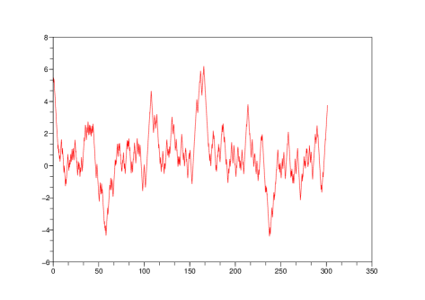
Figure 1: Trajectory of the continuous part $Y$ from the dynamics (1) with $a=1$ and $b=2$.

In this paper, we are interested in the long-time stability properties of the process (1) when $b>a$. One of our motivations is a better understanding of dissipation mechanisms in the setting of hyperbolic equations, where the telegraph process appears as the prototypical associated Markov process. A second motivation is to make a first step in tackling questions on the trend to equilibrium of velocity jump processes introduced in [6], [7], which model the interplay between intra-cellular chemoattractant response mechanisms and collective (macroscopic) behavior of unicellular organisms. These PDMP describe the motion of flagellated bacteria as a sequence of linear “runs”, the directions of which randomly change at rates that evolve according some simple dynamics that represent internal adaptive or excitative responses to chemical changes in the environment (we refer the reader to [20] for a deeper probabilistic description). The emergence of macroscopical drift is expected when the response mechanism favors longer runs in specific directions, and has been numerically confirmed in [6], [7]. In [20], with the aim of developing variance reduction techniques for the numerical simulation of these models, a so-called gradient sensing process was derived from them, in asymptotics where the response mechanisms of bacteria, roughly speaking, act infinitely fast (see Lemma 2.5 in [20] for a precise mathematical statement). The process $(Z_{t})$ above exactly corresponds to the gradient sensing process for the particular chemoattractant potential $S(x)=c|x|\geq 0$ in $\mathbb{R}$, and constitutes a tractable toy model for the long-time behavior of the processes considered in [6], [7], [20] .

When $b>a$ a particle driven by (1) spends in principle more time moving towards the origin than away from it. Thus, a macroscopic attraction to the origin should take place in the long run, though in a consistent way with the fact that the particle has constant speed. Our main goal is to clarify this picture by determining the invariant measure $\mu$ of $(Y,W)$ when $b>a$, and obtaining quantitative bounds (i.e. estimates that are explicit functions of the parameters $a$ and $b$) for the convergence to $\mu$ of the law of $(Y_{t},W_{t})$ as $t$ goes to infinity. Denote by $\|\eta-\tilde{\eta}\|_{\mathrm{TV}}$ the total variation distance between two probability measures $\eta$ and $\tilde{\eta}$ on $\mathbb{R}$ (recalled below at (4)). Our main result is

Theorem 1.1

The invariant probability measure $\mu$ of $(Y,W)$ is the product measure on $\mathbb{R}\times{\left\{-1,+1\right\}}$ given by

$$\mu(dy,dw)=\frac{b-a}{2}e^{-(b-a){\left|y\right|}}dy\otimes\frac{1}{2}(\delta_{-1}+\delta_{+1})(dw).$$

Moreover, denoting by $\mu_{t}^{y,w}$ the law of $Z_{t}=(Y_{t},W_{t})$ when issued from $Z_{0}=(y,w)$, we have, for any $y,\tilde{y}\in\mathbb{R}$ and $w,\tilde{w}\in{\left\{-1,+1\right\}}$,

$${\left\|\mu_{t}^{y,w}-\mu_{t}^{\tilde{y},\tilde{w}}\right\|}_{\mathrm{TV}}\leq C(a,b)e^{r(a,b){\left|y\right|}\vee{\left|\tilde{y}\right|}}e^{-\lambda_{c}t},$$ (2)

where

$$C(a,b)={\left(\frac{b}{a}\right)}^{5/2}\frac{a+b}{\sqrt{ab}+b},\quad r(a,b)=\frac{3(b-a)}{4}\vee(b-\sqrt{ab})\quad\text{and}\quad\lambda_{c}=\frac{(\sqrt{b}-\sqrt{a})^{2}}{2}.$$

We easily deduce

Corollary 1.2

Let $\eta$ be a probability measure in $\mathbb{R}\times{\left\{-1,+1\right\}}$ and let $\mu_{t}^{\eta}$ the law of $Z_{t}$ when the law of $Z_{0}$ is given by $\eta$. Then,

$${\left\|\mu_{t}^{\eta}-\mu\right\|}_{\mathrm{TV}}\leq C(a,b)\int\!e^{r(a,b){\left|y\right|}}\,(\mu+\eta)(dy,dw)e^{-\lambda_{c}t}.$$

The upper bound (2) is integrable under the invariant measure $\mu$ of the full process $(Y,W)$ since $r(a,b)<b-a$. Thus, Corollary 1.2 is significant as soon as $(y,w)\mapsto e^{r(a,b){\left|y\right|}}$ is $\eta$-integrable, ensuring in that case the convergence to equilibrium at exponential rate $\lambda_{c}$. Figure 2 compares the empirical law of $Y_{t}$ to its invariant measure for successive times (the shapes might be compared to those presented in [6, p. 385]).

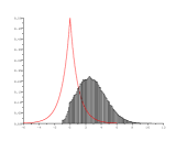
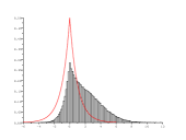
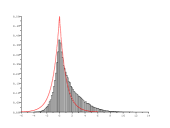
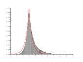
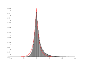
Figure 2: Empirical law of $Y_{t}$ starting at $(5,-1)$ for $t\in{\left\{2,6,10,14,18,22\right\}}$ with $a=1$ and $b=2$.

In spite of the simple form of the process (1), fully explicit computations on this model are not easy to carry out. When $Y_{0}=y>0$, as long as $t<y$ the law of $(Z_{s})_{0\leq s\leq t}$ is equal to the law of the process with generator

$$Hf(y,w)=w\partial_{y}f(y,w)+{\left(a+(b-a)\mathds{1}_{\left\{w>0\right\}}\right)}(f(y,-w)-f(y,w),$$ (3)

which was computed in [9] in terms of modified Bessel functions. We have been unable to compute the transition laws for (1) for general time intervals. (Notice when $a<b$ that long-time behavior of the process driven by (1) is completely different from that of the process driven by (3), which drifts to $-\infty$.)

The proof of the bound in Theorem 1.1 will rely on the construction of a coupling (see [12] and [21] for background), which classically provides a convergence rate to equilibrium depending on tail estimates of the coupling time. A related and popular approach to the long-time behavior of Markov processes is the Foster-Lyapounov-Meyn-Tweedie theory (see [14, 15, 19, 2]), which allows one to prove exponential ergodicity under conditions that are relatively easy to check. Specific applications to PDMP have been developed in [3, 4]. Such general results however provide convergence estimates which are not fully explicit, and sharpness of the bound and rates that can be deduced is hardly assessable.

A fundamental step in proving Theorem 1.1 will be to first establish an analogous result for the reflected (at the origin) version of the process. A fully explicit coupling will be first constructed for the latter, inspired in the coalescent couplings for classic non-negative continuous-time Markov process, namely the M/M/1 queue and reflected Brownian motion with negative drift. The main difficulties in our case are that we have to couple both position and velocity and that, contrary to those examples, we do not have a natural order structure. This prevents us from using the framework developed in [13] to construct couplings for processes that are said to be stochastically ordered.

We will next recall basic ideas employed to study the long time behavior of Markov processes via couplings, following [12]. We also introduce the “reflected version” of the process driven by (1) and state an analogue of Theorem 1.1 for the latter in Theorem 1.4. The strategy of the proofs of Theorems 1.1 and 1.4 together with the structure of the remainder of the paper are then explained. Let us anticipate that the convergence rate $\lambda_{c}$ in (2) will arise as the supremum of the domain of the Laplace transform of the hitting times of origin for the process $(Y_{t})$, suggesting that this rate is sharp. In this direction, we also will see below that in the suitable scaling limit where $(Y_{t})$ converges to the Brownian motion drifted to the origin, the known total variation convergence rate to equilibrium of the latter is recovered as the rescaled limit of the $\lambda_{c}$’s.

1.2 Preliminaries

In all the sequel we will use the notation $\overset{{\mathcal{L}}}{=}$ meaning “equal in law to”. By ${\mathcal{E}}(\lambda)$ and ${\mathcal{P}}(\lambda)$ we will respectively denote the exponential law and the Poisson law of parameter $\lambda>0$, whereas ${\cal B}(p)$ will stand for the Bernoulli distribution of parameter $p\in(0,1)$.

Recall that the total variation distance between two probability measures $\eta$ and $\tilde{\eta}$ in a measurable space ${\mathcal{X}}$ is given by

$${\left\|\eta-\tilde{\eta}\right\|}_{\mathrm{TV}}=\inf{\left\{\mathbb{P}(X\neq\tilde{X})\,:\,X,\tilde{X}\mbox{ random variables with }{\mathcal{L}}(X)=\eta,\ {\mathcal{L}}(\tilde{X})=\tilde{\eta}\right\}},$$ (4)

where each pair of random elements $(X,\tilde{X})$ of ${\mathcal{X}}$ is simultaneously constructed in some probability space and is called a coupling (see [12] for alternative definitions of this distance and its main properties). A coupling $(U_{t},\tilde{U}_{t})_{t\geq 0}$ of two stochastic processes such that $U_{t+T_{*}}=\tilde{U}_{t+T_{*}}$ for any $t\geq 0$ and an almost surely finite random time $T_{*}$ is called a coalescent coupling ($T_{*}$ is then called a coupling time). It follows in this case that

$${\left\|{\mathcal{L}}(U_{t})-{\mathcal{L}}(\tilde{U}_{t})\right\|}_{\mathrm{TV}}\leq\mathbb{P}(T_{*}>t).$$

A helpful notion in obtaining an effective control of the distance is stochastic domination:

Definition 1.3 ([12])

Let $S$ and $T$ be two non-negative random variables with respective cumulative distribution functions $F$ and $G$. We say that $S$ is stochastically smaller than $T$ and we write $S\leq_{\mathrm{sto.}}T$, if $F(t)\geq G(t)$ for any $t\in\mathbb{R}$.

In particular, for a couple $(U_{t},\tilde{U}_{t})$ as above, Chernoff’s inequality yields

$${\left\|{\mathcal{L}}(U_{t})-{\mathcal{L}}(\tilde{U}_{t})\right\|}_{\mathrm{TV}}\leq\mathbb{P}(T>t)\leq\mathbb{E}{\left(e^{\lambda T}\right)}e^{-\lambda t}$$ (5)

for any non-negative random variable $T$ such that $T_{*}\leq_{\mathrm{sto.}}T$, and any $\lambda\geq 0$ in the domain of the Laplace transform $\lambda\mapsto\mathbb{E}{\left(e^{\lambda T}\right)}$ of $T$.

We will use these ideas to obtain the exponential convergence estimates for $Z=(Y,W)$ in Theorem 1.1, and in Theorem 1.4 below for its reflected version $(X,V)$ which we now introduce. The Markov process ${((X_{t},V_{t}))}_{t\geq 0}$ is defined by its infinitesimal generator:

$$Af(x,v)=v\partial_{x}f(x,v)+{\left(a+(b-a)\mathds{1}_{\left\{v>0\right\}}+\frac{\mathds{1}_{\left\{x=0\right\}}}{\mathds{1}_{\left\{x>0\right\}}}\right)}(f(x,-v)-f(x,v)),$$ (6)

with $0<a<b$ (the term $\mathds{1}_{\left\{x=0\right\}}(\mathds{1}_{\left\{x>0\right\}})^{-1}$ means that $X$ is reflected at zero). The dynamics of the process is simple: when $X$ is increasing (resp. decreasing), $V$ flips to $-V$ with rate $b$ (resp. $a)$ and it is reflected in the origin (i.e. as soon as $X=0$, $V$ flips to 1). Given a path ${((Y_{t},W_{t}))}_{t\geq 0}$ driven by (1), a path of ${((X_{t},V_{t}))}_{t\geq 0}$ can be constructed taking

$$X_{t}={\left|Y_{t}\right|},\quad V_{0}=\mathrm{sgn}(Y_{0})W_{0}$$

and defining the set of jump times of $V$ to be

$${\left\{t>0\,:\,\Delta V_{t}\neq 0\right\}}={\left\{t>0\,:\,\Delta W_{t}\neq 0\right\}}\cup{\left\{t>0\,:\,Y_{t}=0\right\}}.$$

Notice that since $W$ does not jump with positive probability when $Y$ hits the origin, one can also construct a path of ${((Y_{t},W_{t}))}_{t\geq 0}$ from an initial value $y\in\mathbb{R}$ and a path ${((X_{t},V_{t}))}_{t\geq 0}$ driven by (6): writing $\sigma_{0}=0$ and ${(\sigma_{i})}_{i\geq 1}$ for the successive hitting times of the origin, we define

$$(Y_{t},W_{t})=(-1)^{i}\mathrm{sgn}(y)(X_{t},V_{t})\quad\text{if }t\in[\sigma_{i},\sigma_{i+1}].$$

Let us state our results about the long time behavior of $(X,V)$.

Theorem 1.4

The invariant measure of $(X,V)$ is the product measure on $\mathbb{R}_{+}\times{\left\{-1,+1\right\}}$ given by

$$\nu(dx,dv)=(b-a)e^{-(b-a)x}\,dx\otimes\frac{1}{2}(\delta_{-1}+\delta_{+1})(dv).$$

If $\nu_{t}^{x,v}$ stands for the law of $(X_{t},V_{t})$ when $X_{0}=x$ and $V_{0}=v$, we have, for any $x,\tilde{x}\geq 0$ and $v,\tilde{v}\in{\left\{-1,+1\right\}}$,

$${\left\|\nu_{t}^{x,v}-\nu_{t}^{\tilde{x},\tilde{v}}\right\|}_{\mathrm{TV}}\leq\frac{(a+b)b}{2a^{2}}e^{r(a,b)(x\vee\tilde{x})}e^{-\lambda_{c}t},$$ (7)

where

$$r(a,b)=\frac{3(b-a)}{4}\vee(b-\sqrt{ab})\quad\text{and}\quad\lambda_{c}=\frac{a+b}{2}-\sqrt{ab}=\frac{(\sqrt{b}-\sqrt{a})^{2}}{2}.$$

Notice that for small times $t\leq{\left|x-\tilde{x}\right|}/2$ the total variation distance does not decrease exponentially fast: the distance between $\nu_{t}^{x,v}$ and $\nu_{t}^{\tilde{x},\tilde{v}}$ is equal to 1 since the supports of these two probability measures are disjoint.

Theorem 1.4 should be compared to results on two classic examples of ergodic non-negative continuous time Markov processes, obtained by coupling arguments that are briefly recalled next. Consider first Brownian motion with negative drift $-c<0$ reflected at the origin and which has the law ${\mathcal{E}}(2c)$ as invariant measure (see [12] for this and the following facts). A coupling of two of its copies $(U^{x}_{t})_{t\geq 0}$ and $(U_{t}^{\tilde{x}})_{t\geq 0}$ respectively starting from $x$ and $\tilde{x}$ consists in letting them evolve independently until they are equal for the first time and choosing them equal from that moment on. By non-negativity and continuity the coupling time $T_{*}$ for $(U^{x}_{t},U_{t}^{\tilde{x}})_{t\geq 0}$ is stochastically smaller that the hitting time $T$ of the origin for ${(U_{t}^{x\vee\tilde{x}})}_{t\geq 0}$. Since for $y>0$ the hitting time $T$ of the origin by $(U^{y}_{t})_{t\geq 0}$ satisfies $\mathbb{E}_{y}{\left(e^{\lambda T}\right)}=\exp{\left(y(c-\sqrt{c^{2}-2\lambda})\right)}$ if $\lambda\in(-\infty,c^{2}/2]$ and $\mathbb{E}_{y}{\left(e^{\lambda T}\right)}=+\infty$ otherwise (see e.g. [17, p. 70]), taking $\lambda=c^{2}/2$ in (5) one gets

$${\left\|{\mathcal{L}}(U^{x}_{t})-{\mathcal{L}}(U^{\tilde{x}}_{t})\right\|}_{\mathrm{TV}}\leq e^{c(x\vee\tilde{x})}e^{-c^{2}t/2}\quad\mbox{ for all }\,x,\tilde{x}\in\mathbb{R}_{+},\,t\geq 0.$$ (8)

This estimate can also be used to study the long time behavior of the solution of the SDE

$$d\xi_{t}=dB_{t}-c\ \mathrm{sgn}(\xi_{t})\,dt$$ (9)

which has the Laplace law $ce^{-2c|x|}dx$ as invariant measure. One first has to couple the absolute values; the first hitting time of the origin after their coupling time stochastically dominates the coupling time for (9). A second example is the M/M/1 queue, that is the continuous time Markov process ${(N_{t})}_{t\geq 0}$ taking values in $\mathbb{N}$ with infinitesimal generator

$$\tilde{A}f(n)=a(f(n+1)-f(n))+b\mathds{1}_{\left\{n>0\right\}}(f(n-1)-f(n))$$

where $b>a>0$ (to ensure ergodicity). Since two independent copies of the process starting from $n$ and $\tilde{n}$ do not jump simultaneously and they have one unit long jumps, their coupling time is smaller than the hitting time of the origin $T$ for the process starting at $n\vee\tilde{n}$. For each initial state $n\in\mathbb{N}$ the Laplace transform of $T$ has domain $(-\infty,(\sqrt{b}-\sqrt{a})^{2}]$ and we have $\mathbb{E}_{n}{\left(e^{(\sqrt{b}-\sqrt{a})^{2}T}\right)}={\left(\frac{b}{a}\right)}^{n/2}$ (see [18] for these facts) which as before yields

$${\left\|{\mathcal{L}}(N^{n}_{t})-{\mathcal{L}}(\tilde{N}^{\tilde{n}}_{t})\right\|}_{\mathrm{TV}}\leq{\left(\frac{b}{a}\right)}^{(n\vee\tilde{n})/2}e^{-(\sqrt{b}-\sqrt{a})^{2}t}\quad\mbox{ for any }n,\tilde{n}\in\mathbb{N},\,t\geq 0.$$

We notice that in the appropriate scaling limit, the M/M/1 queue is furthermore known to converge to the reflected Brownian motion with negative drift (see [18]).

The construction of a coalescent coupling for the process $(X,V)$ driven by (6) is harder than the previous examples since both positions and velocities must be coupled at some time. This will be done in two steps. In Section 3.1 we will obtain an estimate (in the sense of stochastic domination) for the first crossing time and position of $X$ and $\tilde{X}$ for a suitable coupling of the pair. At that time the velocities will be different. We will then construct in Section 3.2 the coalescent coupling when starting from that special configuration. In Section 3.3 we will obtain an explicit upper bound for the Laplace transform of the coalescent time, and thus the quantitative convergence bound (2). The required stochastic dominations will be established in terms of hitting times and lengths of excursions of $(X,V)$ away from the origin. These hitting times will be previously studied in Section 2. We will also give therein a complete description of the excursions and compute thereby the invariant measure of $(X,V)$ using a standard regeneration argument. Finally, Theorem 1.1 will be proved in Section 4 by transferring these results to the unreflected process.

We end this section noting that $\lambda_{c}$ in (2) is the right convergence rate for the process (1), at least in the natural diffusive asymptotics of the process. Let $c>0$ and $0<a_{\scriptscriptstyle N}<b_{\scriptscriptstyle N},N\in\mathbb{N}$ be real numbers. We have

Proposition 1.5

Assume that $a_{\scriptscriptstyle N}+b_{\scriptscriptstyle N}\to\infty$ and $b_{\scriptscriptstyle N}-a_{\scriptscriptstyle N}\to 2c\in(0,\infty)$ as $N\to\infty$. Let $(Y^{({\scriptscriptstyle N})}_{t},W^{({\scriptscriptstyle N})}_{t})_{t\geq 0}$ denote the process driven by (1) with coefficients $a=a_{\scriptscriptstyle N},b=b_{\scriptscriptstyle N}$ and starting from a random variable $Y_{0}^{({\scriptscriptstyle N})}=\xi_{0}\in\mathbb{R}$. Then, as $N\to\infty$, the process

$$\left(\xi^{({\scriptscriptstyle N})}_{t}\right)_{t\geq 0}:=\left(Y^{({\scriptscriptstyle N})}_{t(a_{\scriptscriptstyle N}+b_{\scriptscriptstyle N})/2}\right)_{t\geq 0}$$

converges in law in $C([0,\infty),\mathbb{R})$ to the solution $\xi_{t}$ of the SDE (9) with initial condition $\xi_{0}$.

Remark 1.6

By Theorem 1.1 and the dual representation of the total variation distance,

$$|\mathbb{E}(f(\xi^{({\scriptscriptstyle N}),y}_{t})-\mathbb{E}(f(\xi^{({\scriptscriptstyle N}),\tilde{y}}))|\leq C(a_{\scriptscriptstyle N},b_{\scriptscriptstyle N})e^{r(a_{\scriptscriptstyle N},b_{\scriptscriptstyle N})({\left|y\right|}\vee{\left|\tilde{y}\right|})}\exp\left\{-(a_{\scriptscriptstyle N}+b_{\scriptscriptstyle N})\frac{(\sqrt{b_{\scriptscriptstyle N}}-\sqrt{a_{\scriptscriptstyle N}})^{2}}{4}t\right\}$$

holds for every $t>0$ and each continuous function $f:\mathbb{R}\to[-1,+1]$. Letting $N\to\infty$ and taking then supremum over even functions $f$ in the previous class, we then get that

$${\left\|{\mathcal{L}}(U^{x}_{t})-{\mathcal{L}}(U^{\tilde{x}}_{t})\right\|}_{\mathrm{TV}}\leq e^{3c(x\vee\tilde{x})/2}e^{-c^{2}t/2}\quad\mbox{ for all }\,x,\tilde{x}\in\mathbb{R}_{+},\,t\geq 0,$$

where $(U^{x}_{t})_{t\geq 0}$ and $(U_{t}^{\tilde{x}})_{t\geq 0}$ are Brownian motions with drift $-c<0$ reflected at the origin, respectively starting from $x$ and $\tilde{x}$. Comparison with (8) suggests that the convergence rate $\lambda_{c}$ of Theorem 1.1 cannot be substantially improved on, and that one could in principle improve upon the exponent $r(a,b)$ therein (more precisely, upon the term $3(b-a)/4$).

Proof.

We will use a standard diffusion approximation argument. Omitting for a moment the sub and superscripts for notational simplicity, and writing $j_{t}:=W_{t}-2\kappa W_{t}(a+(b-a)\mathds{1}_{\left\{Y_{t}W_{t}>0\right\}})$, $J_{t}:=\int_{0}^{t}j_{s}ds$ and $\hat{Y}_{t}:=Y_{t}+\kappa W_{t}$ for a given constant $\kappa>0$, we see by Dynkin’s theorem that the processes $M_{t}:=\hat{Y}_{t}-J_{t}$ and $N_{t}:=\hat{Y}_{t}^{2}-t2\kappa-\int_{0}^{t}2Y_{s}j_{s}ds$ are local martingales with respect to the filtration generated by $(Y_{t},W_{t})$. Using integration by parts we then get that $M_{t}^{2}=N_{t}-2\int_{0}^{t}J_{s-}dM_{s}+2\kappa t-2\kappa\int_{0}^{t}W_{s}j_{s}ds$. Thus, noting that $j_{s}=\mathrm{sgn}(Y_{s})\left((2a\kappa-1)+2\times\mathds{1}_{\left\{Y_{s}W_{s}>0\right\}}(1-\kappa(b+a))\right)$, we see for $\kappa=(a+b)^{-1}$ that

$$M_{t}=Y_{t}-\left[\int_{0}^{t}\mathrm{sgn}(Y_{s})\left(\frac{a-b}{a+b}\right)ds-\frac{W_{t}}{a+b}\right]\,,\,M_{t}^{2}-\left[\frac{2t}{a+b}-2\int_{0}^{t}W_{s}\,\mathrm{sgn}(Y_{s})\frac{a-b}{(a+b)^{2}}ds\right]$$

are local martingales. Therefore, defining for each $N\in\mathbb{N}$

$$\beta^{({\scriptscriptstyle N})}_{t}:=\frac{(a_{\scriptscriptstyle N}-b_{\scriptscriptstyle N})}{2}\int_{0}^{t}\mathrm{sgn}(\xi_{s}^{({\scriptscriptstyle N})})ds-\frac{W^{({\scriptscriptstyle N})}_{t(a_{\scriptscriptstyle N}+b_{\scriptscriptstyle N})/2}}{a_{\scriptscriptstyle N}+b_{\scriptscriptstyle N}}$$

and

$$\alpha^{({\scriptscriptstyle N})}_{t}:=t-\frac{(a_{\scriptscriptstyle N}-b_{\scriptscriptstyle N})}{a_{\scriptscriptstyle N}+b_{\scriptscriptstyle N}}\int_{0}^{t}W^{({\scriptscriptstyle N})}_{s(a_{\scriptscriptstyle N}+b_{\scriptscriptstyle N})/2}\,\mathrm{sgn}(\xi_{s}^{({\scriptscriptstyle N})})ds\,,$$

we readily check that the processes $\xi^{({\scriptscriptstyle N})}_{t},\alpha^{({\scriptscriptstyle N})}_{t}$ and $\beta^{({\scriptscriptstyle N})}_{t}$ satisfy assumptions (4.1) to (4.7) of Theorem 4.1 in [8, p. 354] (in the respective roles of the processes $X_{n}(t),A_{n}(t)$ and $B_{n}(t)$ therein). That result ensures that ${\mathcal{L}}(\xi^{({\scriptscriptstyle N})})$ converges weakly to the unique solution of the martingale problem with generator $Gf(x):=\frac{1}{2}f^{\prime\prime}(x)-c\,\mathrm{sgn}(x)f^{\prime}(x),f\in C_{c}^{\infty}(\mathbb{R})$ and initial law ${\mathcal{L}}(\xi_{0})$. ∎

2 The invariant measure of the reflected process

In this section we will determine the invariant measure of $(X,V)$. This process is clearly positive recurrent since, as will be shown in the sequel, the Laplace transform of the hitting time of $(0,+1)$ is finite on a neighborhood of the origin, whatever the initial data are. We will need the following well-known results for Poisson processes.

Proposition 2.1 ([16])

Let ${(N_{t})}_{t\geq 0}$ be a Poisson process with intensity $\lambda>0$. Denote by ${(T_{n})}_{n\geq 1}$ its jump times. Then, $N_{t}\sim{\mathcal{P}}(\lambda t)$ for any $t\geq 0$. Moreover, conditionally on ${\left\{N_{t}=k\right\}}$, the jump times $T_{1},T_{2},\ldots,T_{k}$ have the same distribution than an ordered sample of size $k$ from the uniform distribution on $[0,t]$.

2.1 Excursion and hitting times

We start by computing the Laplace transforms of the length of an excursion (to be defined next) and of the hitting times of the origin when starting from $(x,v)\in\mathbb{R}_{+}\times{\left\{-1,+1\right\}}$.

Definition 2.2

An excursion of $(X,V)$ driven by (6) is a path starting at $(0,+1)$ and stopped at

$$S=\inf{\left\{t>0\,:\,X_{t}=0\right\}}.$$

We denote by $\psi$ the Laplace transform of $S$:

$$\psi\,:\,\lambda\in\mathbb{R}\mapsto\psi(\lambda)=\mathbb{E}_{(0,+1)}{\left(e^{\lambda S}\right)}.$$ (10)

Notice that $\lim_{t\rightarrow S^{-}}V_{t}=-1$ and $V_{S}=1$.

Lemma 2.3 (Length of an excursion.)

The domain of $\psi$ defined in (10) is equal to $(-\infty,\lambda_{c}]$ where

$$\lambda_{c}=\frac{a+b}{2}-\sqrt{ab}=\frac{(\sqrt{b}-\sqrt{a})^{2}}{2}.$$ (11)

Furthermore, if $\lambda\leq\lambda_{c}$,

$$\psi(\lambda)=\frac{a+b-2\lambda-\sqrt{(a+b-2\lambda)^{2}-4ab}}{2a}.$$ (12)

In particular, $\psi(\lambda_{c})=\sqrt{b/a}$ and $\mathbb{E}_{(0,+1)}(S)=2/(b-a)$.

Proof.

During a time length $E$ of law ${\mathcal{E}}(b)$, $V$ is equal to 1 and $X$ grows linearly. At time $t=E$, $V$ flips to $-1$ and $X$ starts going down. Denote by $T_{2}$ the second jump time of $V$. If $X_{T_{2}}=0$, then $S=2E$. Otherwise, $X$ starts a new excursion above $X_{T_{2}}$ which has the same law as $S$ and is independent of the past. After this excursion, $(X,V)$ is equal to $(X_{T_{2}},-1)$. Once again, it reaches 0 directly or $V$ flips to 1 before doing so, in which case a new independent excursion begins. Proposition 2.1 and the strong Markov property ensure that, conditionally on ${\left\{E=x\right\}}$, the number $N$ of embedded excursions has the law ${\mathcal{P}}(ax)$. We thus can decompose $S$ as

$$S\overset{{\mathcal{L}}}{=}2E+\sum_{k=1}^{N}S_{k},$$

where $E\sim{\mathcal{E}}(b)$, ${\mathcal{L}}(N|E=x)={\mathcal{P}}(ax)$ and ${(S_{k})}_{k\geq 1}$ is an i.i.d. sequence of random variables distributed as $S$ and independent of the couple $(E,N)$. As a consequence,

$$\psi(\lambda) =\mathbb{E}{\left(\mathbb{E}{\left(e^{2\lambda E+\lambda\sum_{k=1}^{N}S_{k}}|E,N\right)}\right)}=\mathbb{E}{\left(e^{2\lambda E}\mathbb{E}{\left(\psi(\lambda)^{N}|E\right)}\right)}$$

$$=\mathbb{E}{\left(e^{2\lambda E}e^{aE(\psi(\lambda)-1)}\right)}=\frac{b}{b+a-2\lambda-a\psi(\lambda)}$$

for each $\lambda$ in the domain of $\psi$ (which contains $(-\infty,0]$). This implies (since $\psi$ is a Laplace transform) that

$$\psi(\lambda)=\frac{a+b-2\lambda-\sqrt{(a+b-2\lambda)^{2}-4ab}}{2a}.$$

The relation is in fact valid as soon as the argument of the square root is non-negative i.e. as soon as $\lambda\leq\lambda_{c}$ with $\lambda_{c}$ defined in (11). At last, $\mathbb{E}_{(0,+1)}(S)=\psi^{\prime}(0)=2/(b-a)$. ∎

Remark 2.4 (Number of jumps in an excursion)

Since each excursion is preceded by a jump, the number $M$ of jumps of $V$ during an excursion (omitting the jump at time $S$) satisfies

$$M\overset{{\mathcal{L}}}{=}1+\sum_{i=1}^{N}(1+M_{i})$$

where ${(M_{i})}_{i\geq 0}$ is an i.i.d. sequence with the same law as $M$ and independent of the random variable $N$ such that ${\mathcal{L}}(N|E)={\mathcal{P}}(aE)$ with $E\sim{\mathcal{E}}(b)$. By conditioning first in $E,N$ as in the previous proof, one can easily derive a second degree equation and then an explicit expression for the Laplace transform of the number of jumps. We omit the details since this result will not be needed.

Lemma 2.5

For $x>0$, let $S_{(x,-1)}$ denote the hitting time of 0 starting from $(x,-1)$. Then

$$\mathbb{E}{\left(e^{\lambda S_{(x,-1)}}\right)}=e^{xc(\lambda)}\quad\text{with}\quad c(\lambda)=\frac{b-a-\sqrt{(a+b-2\lambda)^{2}-4ab}}{2}$$ (13)

if $\lambda\in(-\infty,\lambda_{c}]$, and $+\infty$ otherwise.

Proof.

As in the proof of Lemma 2.3, one can decompose $S_{(x,-1)}$ as

$$S_{(x,-1)}\overset{{\mathcal{L}}}{=}x+\sum_{k=1}^{N}S_{k},$$

where $N$ is a random variable with law ${\mathcal{P}}(ax)$ independent of the i.i.d. sequence of random variables ${(S_{k})}_{k\geq 1}$ with Laplace transform $\psi$. Then,

$$\mathbb{E}{\left(e^{\lambda S_{(x,-1)}}\right)}=\sum_{k\geq 1}\mathbb{E}{\left(e^{\lambda(x+S_{1}+S_{2}+\cdots+S_{k})}\mathds{1}_{\left\{N=k\right\}}\right)}=e^{ax(\psi(\lambda)-1)+\lambda x}.$$

At last, $a(\psi(\lambda)-1)+\lambda$ is equal to $c(\lambda)$. ∎

Corollary 2.6

For any $x\geq 0$, let us denote by $S_{(x,+1)}$ the hitting time of 0 starting from $(x,+1)$. Then

$$\mathbb{E}{\left(e^{\lambda S_{(x,+1)}}\right)}=\psi(\lambda)e^{xc(\lambda)},$$

where $\psi$ is given by (12) and $c(\lambda)$ by (13).

Proof.

The strong Markov property implies that $S_{(x,+1)}\overset{{\mathcal{L}}}{=}S+S_{(x,-1)}$ where $S$ is the length of an excursion independent from $S_{(x,-1)}$. ∎

Lemma 2.7

For any $x,\tilde{x}\geq 0$,

$$S_{(x+\tilde{x},-1)}\overset{{\mathcal{L}}}{=}S_{(x,-1)}+S_{(\tilde{x},-1)}\geq_{\mathrm{sto.}}S_{(x,-1)},$$

where $S_{(x,-1)}$ and $S_{(\tilde{x},-1)}$ are independent.

Proof.

This is a straightforward consequence of the strong Markov property. ∎

2.2 The invariant measure

Recall that the invariant law of $(X,V)$ is denoted by $\nu$.

Lemma 2.8

For any bounded function $f:\mathbb{R}\times{\left\{-1,+1\right\}}\to\mathbb{R}$, we have

$$\int\!f\,d\nu=\frac{1}{\mathbb{E}_{(0,+1)}(S)}\mathbb{E}_{(0,+1)}{\left(\int_{0}^{S}\!f(X_{s},V_{s})\,ds\right)},$$

where $S$ is the first hitting time of 0.

Proof.

We will use a standard result on regenerative processes (see Asmussen [1, Chapter VI] for background). Let $(S_{n})_{n\geq 1}$ denote the lengths of the consecutive excursions away from $0$, $S_{0}:=S$ and $\Theta_{n}:=S_{0}+\dots+S_{n}$. By the strong Markov property, $(\Theta_{n})_{n\in\mathbb{N}}$ is a renewal process, for each $n\in\mathbb{N}$ the post $\Theta_{n}$-process $(\Theta_{n+1},\Theta_{n+2},\dots,(X_{\Theta_{n}+t},V_{\Theta_{n}+t})_{t\geq 0})$ is independent of $(\Theta_{0},\dots,\Theta_{n})$, and is equally distributed for all $n\geq 1$. This means that $(X_{t},V_{t})_{t\geq 0}$ is a regenerative process with regeneration points $(\Theta_{n})_{n\in\mathbb{N}}$ and cycle length corresponding to the length of an excursion. The result is immediate from [1, Theorem 1.2, Chapter VI] and Lemma 2.3. ∎

Lemma 2.9

Define, for a non negative function $g:{\left\{-1,+1\right\}}\to\mathbb{R}$ and $\lambda\in\mathbb{R}$,

$$F:=\int_{0}^{S}e^{\lambda X_{s}}g(V_{s})\,ds.$$

Then, conditionally on $(X_{0},V_{0})=(0,+1)$, we have

$$F\overset{{\mathcal{L}}}{=}(g(1)+g(-1))\int_{0}^{E}\!e^{\lambda y}\,dy+\sum_{i=1}^{N}\int_{0}^{S^{(i)}}\!e^{\lambda(EU_{(i,N)}+X^{(i)}_{s})}g(V^{(i)}_{s})\,ds,\mbox{ where }$$

• ${(U_{i})}_{i\geq 0}$ is an sequence of independent uniformly distributed random variables on $[0,1]$, and for each $n\geq 1$ $(U_{(1,n)},U_{(2,n)},\ldots,U_{(n,n)})$ is the re-ordered sampling of $(U_{1},U_{2},\ldots,U_{n})$;

• ${(X^{(i)}_{t},V^{(i)}_{t})}_{0\leq t\leq S^{(i)}}$ is a sequence of independent excursions;

• $E\sim{\mathcal{E}}(b)$, ${\mathcal{L}}(N|E=x)={\mathcal{P}}(ax)$, and the pair $(E,N)$ is independent of the all the previous random variables.

Proof.

The argument has been already been given in the first part of the proof of Lemma 2.3. We just notice that the $N$ independent embedded excursions therein occur at the heights $(EU_{(N,N)},EU_{(N-1,N)},\ldots,EU_{(1,N)})$ (see Proposition 2.1). ∎

We now are ready to compute $\nu$ which is the first point in Theorem 1.4. Since

$$\mathbb{E}{\left(\int_{0}^{S^{(i)}}\!e^{\lambda(EU_{(i,N)}+X^{(i)}_{s})}g(V^{(i)}_{s})\,ds\Big{|}E,N,{(U_{i})}_{i\geq 1}\right)}=e^{\lambda EU_{(i,N)}}\mathbb{E}_{(0,+1)}(F),$$

we get that

$$\mathbb{E}_{(0,+1)}(F)=\mathbb{E}{\left(\frac{(g(1)+g(-1))}{\lambda}(e^{\lambda E}-1)+\mathbb{E}_{(0,+1)}(F)\sum_{i=1}^{N}e^{\lambda EU_{(i,N)}}\right)}.$$

We have, for any $x>0$ and $k\in\mathbb{N}$,

$$\sum_{i=1}^{k}\mathbb{E}{\left(e^{\lambda xU_{(i,k)}}\right)}=\mathbb{E}{\left(\sum_{i=1}^{k}e^{\lambda xU_{i}}\right)}=\frac{k}{\lambda x}(e^{\lambda x}-1),$$

and then

$$\mathbb{E}{\left(\sum_{i=1}^{N}e^{\lambda EU_{(i,N)}}\Big{|}E\right)}=\mathbb{E}{\left(\frac{N}{\lambda E}(e^{\lambda E}-1)\Big{|}E\right)}=\frac{a}{\lambda}(e^{\lambda E}-1).$$

As a conclusion, we have

$$\mathbb{E}_{(0,+1)}(F) =\frac{g(1)+g(-1)+a\mathbb{E}_{(0,+1)}(F)}{\lambda}{\left(\frac{b}{b-\lambda}-1\right)}$$

$$=\frac{g(1)+g(-1)}{b-\lambda}+\frac{a}{b-\lambda}\mathbb{E}_{(0,+1)}(F),$$

which provides the expression of $\mathbb{E}_{(0,+1)}(F)$ for any $\lambda<b-a$:

$$\mathbb{E}_{(0,+1)}(F)=\frac{g(1)+g(-1)}{b-a-\lambda}.$$

On the other hand, Lemma 2.3 ensures that $\mathbb{E}_{(0,+1)}(S)=2/(b-a)$ from where we get, for any $\lambda<b-a$, that

$$\int_{\mathbb{R}\times{\left\{-1,+1\right\}}}\!e^{\lambda x}g(v)\nu(dx,dv)=\frac{b-a}{b-a-\lambda}\frac{g(1)+g(-1)}{2}.$$

In other words, the invariant measure of $(X,V)$ is $\nu={\mathcal{E}}(b-a)\otimes(1/2)(\delta_{-1}+\delta_{+1})$.

3 The coalescent time for the reflected process

3.1 The crossing time

We will first construct a coupling $(X,V,\tilde{X},\tilde{V})$ starting at $(x,v,\tilde{x},\tilde{v})$ until a time $T_{c}=T_{c}(x,v,\tilde{x},\tilde{v})$ called crossing time, at which $X_{T_{c}}=\tilde{X}_{T_{c}}$. In doing so, we will also stochastically control $T_{c}$ and $X_{T_{c}}$. The coupling will consist in making the two velocities equal as longer as possible. Assume without loss of generality that $\tilde{x}<x$. Plainly, if $V$ and $\tilde{V}$ are different, we let the two processes evolve independently until one of them performs a jump or until $X-\tilde{X}$ hits $0$. At that time, if $X\neq\tilde{X}$, the two velocities are equal and we set them equal until $\tilde{X}$ hits the origin. During this period the paths of $X$ and $\tilde{X}$ are parallel and, at the hitting time of the origin, $V$ and $\tilde{V}$ are once again different. We then iterate this procedure until $T_{c}$. Notice that $\tilde{X}$ is smaller than $X$ on $[0,T_{c})$. We now make the construction with full details.

3.1.1 The main initial configuration

Assume first that $(X_{0},V_{0},\tilde{X}_{0},\tilde{V}_{0})=(x,-1,0,+1)$. The coupling works as follows: with rate $a$ (resp. $b$), $V$ (resp. $\tilde{V}$) flips to $+1$ (resp. $-1$) and if none of these two events occurs before time $x/2$, then

$$X_{x/2}=\tilde{X}_{x/2}\quad\text{and}\quad V_{x/2}=-1=-\tilde{V}_{x/2}.$$

If a jump occurs at time $\tau_{1}<x/2$, then $(X_{\tau_{1}},V_{\tau_{1}},\tilde{X}_{\tau_{1}},\tilde{V}_{\tau_{1}})=(x-\tau_{1},U,\tau_{1},U)$, where $U=-1$ with probability $b/(a+b)$ ($\tilde{V}$ jumps before $V$) and $U=1$ with probability $a/(a+b)$. Then, $V$ and $\tilde{V}$ are chosen equal until $\tilde{X}$ hits 0 i.e. during a time $S_{(\tau_{1},U)}$ and

$$(X_{\tau_{1}+S_{(\tau_{1},U)}},V_{\tau_{1}+S_{(\tau_{1},U)}},\tilde{X}_{\tau_{1}+S_{(\tau_{1},U)}},\tilde{V}_{\tau_{1}+S_{(\tau_{1},U)}})=(x-2\tau_{1},-1,0,+1).$$

Notice that $S_{(\tau_{1},+1)}\overset{{\mathcal{L}}}{=}S+S_{(\tau_{1},-1)}$ where $S$ is the length of an excursion independent of $S_{(\tau_{1},-1)}$. As a conclusion, if a jump occurs at time $\tau_{1}<x/2$, then the full process $(X,V,\tilde{X},\tilde{V})$ is equal to $(x-2\tau_{1},-1,0,+1)$ at time $\tau_{1}+S_{(\tau_{1},-1)}+BS$ where $B\sim{\mathcal{B}}(a/(a+b))$. One has to iterate this procedure until $X-\tilde{X}$ hits 0.

Consider now a Poisson process ${(N(t))}_{t\geq 0}$ with intensity $a+b$. We denote by ${(T_{n})}_{n\geq 0}$ its jump times (with $T_{0}=0$) and define ${(\tau_{i})}_{i\geq 1}$ by $\tau_{i}=T_{i}-T_{i-1}$ for $i\geq 1$. The number of return times at 0 for $\tilde{X}$ before $T_{c}$ is distributed as $N(x/2)$ and the length of the periods when $(X,V)$ and $(\tilde{X},\tilde{V})$ are independent are given by $\tau_{1}$, $\tau_{2}$,…,$\tau_{N(x/2)}$ and $x/2-T_{N(x/2)}$. Then,

$$T_{c}(x,-1,0,+1)\overset{{\mathcal{L}}}{=}\sum_{i=1}^{N(x/2)}{\left(\tau_{i}+S_{(\tau_{i},-1)}+B_{i}S^{(i)}\right)}+x/2-T_{N(x/2)},$$

where the law of ${(S^{(i)})}_{i\geq 1}$ is the one of the length of an excursion, ${(S_{(\tau_{i},-1)})}_{i\geq 1}$ are the hitting times of 0 starting from ${(\tau_{i})}_{i\geq 1}$, ${(B_{i})}_{i\geq 1}$ have the law ${\mathcal{B}}(a/(a+b))$ and all these random variables are independent. Since $T_{N(x/2)}=\tau_{1}+\tau_{2}+\cdots+\tau_{N(x/2)}$, Lemma 2.7 ensures that

$$T_{c}(x,-1,0,+1) \overset{{\mathcal{L}}}{=}x/2+S_{(T_{N(x/2)},-1)}+\sum_{i=1}^{N(x/2)}{\left(B_{i}S^{(i)}\right)}$$

$$\leq_{\mathrm{sto.}}x/2+S_{(x/2,-1)}+\Sigma(x)$$ (14)

where

$$\Sigma(x):\overset{{\mathcal{L}}}{=}\sum_{i=1}^{N(x/2)}{\left(B_{i}S^{(i)}\right)}.$$

Notice that $\Sigma(u+v)\overset{{\mathcal{L}}}{=}\Sigma(u)+\Sigma(v)$, where $\Sigma(u)$ and $\Sigma(v)$ are independent, and that $\Sigma(u)$ distributes as the sum of the lengths of $N$ independent excursions, with $N\sim{\mathcal{P}}(au/2)$.

3.1.2 Other configurations

We next construct the paths until $T_{c}(x,v,\tilde{x},\tilde{v})$ and control this time irrespective of the initial velocities. Without loss of generality, we can assume that $x\geq\tilde{x}$. We just have to construct the paths until $(X,V,\tilde{X},\tilde{V})$ reaches a state $(u,-1,0,+1)$, and then make use of the previous section.

Assume firstly that $v=\tilde{v}=U\in{\left\{-1,+1\right\}}$. We have to construct a trajectory of $(\tilde{X},\tilde{V})$ until $S_{(\tilde{x},U)}$ the hitting time of $0$. Define for any $t\in[0,S_{(\tilde{x},U)})$, $V_{t}=\tilde{V}_{t}$, $X_{t}=\tilde{X}_{t}-\tilde{x}+x$, $V_{S_{(\tilde{x},U)}}=-1$ and $X_{S_{(\tilde{x},U)}}=x-\tilde{x}$. Using Lemma 2.7 and (3.1.1), one has

$$T_{c}(x,U,\tilde{x},U) \overset{{\mathcal{L}}}{=}S_{(\tilde{x},U)}+T_{c}(x-\tilde{x},-1,0,+1)$$

$$\overset{{\mathcal{L}}}{=}S\mathds{1}_{\left\{U=+1\right\}}+S_{(\tilde{x},-1)}+T_{c}(x-\tilde{x},-1,0,+1)$$

$$\leq_{\mathrm{sto.}}S\mathds{1}_{\left\{U=+1\right\}}+\frac{x-\tilde{x}}{2}+S_{((x+\tilde{x})/2,-1)}+\Sigma(x-\tilde{x}).$$

Assume now that $v=1=-\tilde{v}$. The processes $(X,V)$ and $(\tilde{X},\tilde{V})$ are chosen independent until the first jump time. This is equal to $E=(E_{1}\wedge\tilde{x})\wedge E_{2}$, where $E_{1}\sim{\mathcal{E}}(a)$, $E_{2}\sim{\mathcal{E}}(b)$ and $(X_{E},V_{E},\tilde{X}_{E},\tilde{V})=(x+E,U,\tilde{x}-E,U)$ with $U\in{\left\{-1,+1\right\}}$. In particular, one has

$$\frac{X_{E}+\tilde{X}_{E}}{2}=\frac{x+\tilde{x}}{2}\quad\text{and}\quad\frac{X_{E}-\tilde{X}_{E}}{2}=\frac{x-\tilde{x}}{2}+E.$$

Since for any $y,\tilde{y}\geq 0$, $T_{c}(y,-1,\tilde{y},-1)\leq_{\mathrm{sto.}}T_{c}(y,1,\tilde{y},1)$ this ensures that

$$T_{c}(x,+1,\tilde{x},-1) \leq_{\mathrm{sto.}}E+T_{c}(x+E,+1,\tilde{x}-E,+1)$$

$$\leq_{\mathrm{sto.}}E+S+\frac{x-\tilde{x}}{2}+E+S_{((x+\tilde{x})/2,-1)}+\Sigma(x-\tilde{x}+2E)$$

$$\leq_{\mathrm{sto.}}2E+\Sigma(2E)+S+\frac{x-\tilde{x}}{2}+S_{((x+\tilde{x})/2,-1)}+\Sigma(x-\tilde{x}).$$

If $v=-1=-\tilde{v}$, we proceed as in the previous case. With the same notations,

$$\frac{X_{E}+\tilde{X}_{E}}{2}=\frac{x+\tilde{x}}{2}\quad\text{and}\quad\frac{|X_{E}-\tilde{X}_{E}|}{2}\leq\frac{x-\tilde{x}}{2}+E.$$

We then get the same upper bound as before. As a conclusion we have established the following upper bound for $T_{c}$:

Lemma 3.1

For any $x\geq\tilde{x}$ and $v,\tilde{v}\in{\left\{-1,+1\right\}}$,

$$T_{c}(x,v,\tilde{x},\tilde{v})\leq_{\mathrm{sto.}}2E+\Sigma(2E)+S+S_{((x+\tilde{x})/2,-1)}+\frac{x-\tilde{x}}{2}+\Sigma(x-\tilde{x}),$$

where $E=F\wedge\tilde{x}$ with $F$ is an exponential variable with parameter $a+b$ and $\Sigma(u)$ is the sum of the lengths of $N$ independent excursions where $N\sim{\mathcal{P}}(au/2)$. Moreover,

$$X_{T_{c}}=\tilde{X}_{T_{c}}\leq\frac{x-\tilde{x}}{2}+E\quad\text{and}\quad V_{T_{c}}=-\tilde{V}_{T_{c}}.$$

3.2 A simple way to stick the paths

We now assume that $(X_{0},V_{0})=(x,1)$ and $(\tilde{X}_{0},\tilde{V}_{0})=(x,-1)$ and construct two paths which are equal after a coalescent time $T_{cc}(x)$. The idea is to use the same exponential clocks for both paths but in a different order. We explain the generic step of this construction considering $R$ and $Q$ two given independent random variables with respective laws ${\mathcal{E}}(a)$ and ${\mathcal{E}}(b)$. There are two possible situations:

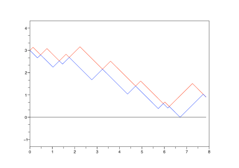
Figure 3: Two paths starting at $x=3$ with different velocities until they stick together.

• Case 1: $R<x$. In this case, defining $T=R+Q$,

  $$V_{t}=\begin{cases}+1&\text{if }t\in[0,Q),\\ -1&\text{if }t\in[Q,T),\\ +1&\text{if }t=T\end{cases}\quad\text{and}\quad\tilde{V}_{t}=\begin{cases}-1&\text{if }t\in[0,R),\\ +1&\text{if }t\in[R,T),\\ -1&\text{if }t=T,\end{cases}$$

  one has $X_{T}=x+Q-R=\tilde{X}_{T}$ and $V_{T}=1=-\tilde{V}_{T}$.

• Case 2: $R\geq x$. In this case, defining $T=x+Q$,

  $$V_{t}=\begin{cases}+1&\text{if }t\in[0,Q),\\ -1&\text{if }t\in[Q,T),\end{cases}\quad\text{and}\quad\tilde{V}_{t}=\begin{cases}-1&\text{if }t\in[0,x),\\ +1&\text{if }t\in[x,T),\\ -1&\text{if }t=T,\end{cases}$$

  one has $X_{T}=Q=\tilde{X}_{T}$ and $V_{T}=\tilde{V}_{T}=-1$. In this case $(X,V)$ and $(\tilde{X},\tilde{V})$ are coupled at time $T$.

We now construct the paths. We take an i.i.d. sequence of independent pairs of exponential variables $(R_{n},Q_{n})$ with $R_{n}\sim{\mathcal{E}}(a)$ and $Q_{n}\sim{\mathcal{E}}(b)$, and inductively define $\tau_{0}=0$ and $\tau_{n+1}=\tau_{n}+T_{n}$, with $T_{n}$ defined from $(R_{n},Q_{n})$ as above until Case 2 occurs. At each iteration,

• if $\tilde{X}$ does not hit the origin in the interval $[\tau_{n},\tau_{n+1}]$ (Case 1) we set

  $$X_{\tau_{n+1}}=\tilde{X}_{\tau_{n+1}}\quad\text{and}\quad V_{\tau_{n+1}}=1=-\tilde{V}_{\tau_{n+1}}\,;$$

• if $\tilde{X}$ hits the origin in the interval $[\tau_{n},\tau_{n+1}]$ (Case 2) we set

  $$X_{\tau_{n+1}}=\tilde{X}_{\tau_{n+1}}\quad,\quad V_{\tau_{n+1}}=\tilde{V}_{\tau_{n+1}}=-1\quad\text{and}\quad T_{cc}(x):=\tau_{n+1}.$$

By construction, $X_{t}\geq\tilde{X}_{t}$ for any $t\geq 0$ and the coupling time $T_{cc}(x)$ is smaller than the hitting time of the origin time of $X$ (see Figure 3). As a conclusion we have shown the following result.

Lemma 3.2

There exists a coupling of $(X,V)$ and $(\tilde{X},\tilde{V})$ starting respectively from $(x,1)$ and $(x,-1)$ such that the coalescent time $T_{cc}(x)$ is (stochastically) smaller than $S_{(x,+1)}$ and

$$X_{S_{(x,+1)}}=\tilde{X}_{S_{(x,+1)}}=0\quad\text{and}\quad V_{S_{(x,+1)}}=\tilde{V}_{S_{(x,+1)}}=1.$$

3.3 The Laplace transform of the coupling time

We now gather the previous estimates to control the Laplace transform of the coupling time of the two paths starting respectively from $(x,v)$ and $(\tilde{x},\tilde{v})$:

Proposition 3.3

For any $x\geq\tilde{x}\geq 0$, any $v,\tilde{v}\in{\left\{-1,+1\right\}}$, there exists a coalescent coupling such that the coupling time $T(x,v,\tilde{x},\tilde{v})$ is stochastically smaller than a random variable

$$\overline{T}(x,\tilde{x})\overset{{\mathcal{L}}}{=}F+\Sigma(2F)+S_{(F,-1)}+S+\tilde{S}+S_{(x,-1)}+\frac{x+\tilde{x}}{2}+\Sigma(x-\tilde{x}),$$ (15)

where $F\sim{\mathcal{E}}(a+b)$, $S$ and $\tilde{S}$ are excursion lengths and all the random variables are independent. Furthermore, for any $\lambda\in[0,\lambda_{c}]$,

$$\mathbb{E}{\left(e^{\lambda T(x,v,\tilde{x},\tilde{v})}\right)}\leq\frac{(a+b)\psi(\lambda)^{2}}{2a+b-\lambda-a\psi(\lambda)-c(\lambda)}\exp{\left(xc(\lambda)+\frac{x+\tilde{x}}{2}\lambda+\frac{x-\tilde{x}}{2}a(\psi(\lambda)-1)\right)}.$$

At last, a realization of $\bar{T}(x,\tilde{x})$ is the first hitting time at $0$ of $X$ after $T_{c}(x,v,\tilde{x},\tilde{v})+T_{cc}(X_{T_{c}(x,v,\tilde{x},\tilde{v}})$, and then $X_{\overline{T}(x,\tilde{x})}=\tilde{X}_{\overline{T}(x,\tilde{x})}=0$ and $V_{\overline{T}(x,\tilde{x})}=\tilde{V}_{\overline{T}(x,\tilde{x})}=1$ hold.

Proof.

From the previous sections, one can construct a coalescent coupling with a coalescent time $T$ such that

$$T(x,v,\tilde{x},\tilde{v})\overset{{\mathcal{L}}}{=}T_{c}(x,v,\tilde{x},\tilde{v})+T_{cc}(X_{T_{c}(x,v,\tilde{x},\tilde{v})}).$$

Thanks to Lemmas 2.7, 3.1 and 3.2, we get that

$$T(x,v,\tilde{x},\tilde{v}) \leq_{\mathrm{sto.}}2E+\Sigma(2E)+S+S_{((x+\tilde{x})/2,-1)}+\frac{x-\tilde{x}}{2}+S_{((x-\tilde{x})/2+E,+1)}+\Sigma(x-\tilde{x})$$

$$\leq_{\mathrm{sto.}}2E+\Sigma(2E)+S_{(E,-1)}+S+\tilde{S}+S_{(x,-1)}+\frac{x-\tilde{x}}{2}+\Sigma(x-\tilde{x}),$$

where $\tilde{S}$ is an independent copy of $S$ and all the random variables of the right hand side are independent. Recall that $E$ is equal to $F\wedge\tilde{x}$ where $F$ is a random variable variable of law ${\mathcal{E}}(a+b)$. In particular, $2E\leq_{\mathrm{sto.}}F+\tilde{x}$ and then

$$T(x,v,\tilde{x},\tilde{v})\leq_{\mathrm{sto.}}\overline{T}(x,\tilde{x}),$$

where $\overline{T}(x,\tilde{x})$ is given by (15). At last, for any $\lambda\leq\lambda_{c}$, one has

$$\lambda+a(\psi(\lambda)-1)+c(\lambda)\leq\lambda_{c}+a(\psi(\lambda_{c})-1)+c(\lambda_{c})=b-a<a+b.$$

This ensures that for any $\lambda\leq\lambda_{c}$,

$$\mathbb{E}{\left(e^{\lambda F+\lambda\Sigma(2F)+\lambda S_{(F,-1)}}\right)} =\mathbb{E}{\left(e^{(\lambda+a(\psi(\lambda)-1)+c(\lambda))F}\right)}=\frac{a+b}{2a+b-\lambda-a\psi(\lambda)-c(\lambda)}.$$

Using the independence of the random variables provides the desired upper bound. ∎

Corollary 3.4

In particular, if $\tilde{x}\leq x$,

$$\mathbb{E}{\left(e^{\lambda_{c}T(x,v,\tilde{x},\tilde{v})}\right)}\leq\frac{(a+b)b}{2a^{2}}e^{r(a,b)x},$$

where $\lambda_{c}$ is given in (11) and

$$r(a,b)=\frac{3(b-a)}{4}\vee(b-\sqrt{ab}).$$

Proof.

Let us choose $\lambda=\lambda_{c}$. Since

$$\lambda_{c}=\frac{(\sqrt{b}-\sqrt{a})^{2}}{2},\quad c(\lambda_{c})=\frac{b-a}{2}\quad\text{and}\quad\psi(\lambda_{c})=\sqrt{\frac{b}{a}},$$

we get that

$$xc(\lambda_{c})+\frac{x+\tilde{x}}{2}\lambda_{c}+\frac{x-\tilde{x}}{2}a(\psi(\lambda_{c})-1)=\frac{\sqrt{b}-\sqrt{a}}{4}{\left(3x(\sqrt{b}+\sqrt{a})+\tilde{x}(\sqrt{b}-3\sqrt{a})\right)}.$$

If $x$ is fixed, then the right hand side is a linear function of $\tilde{x}\in[0,x]$ and it is bounded above by the maximum of its values at $\tilde{x}\in{\left\{0,x\right\}}$. In other words,

$$xc(\lambda)+\frac{x+\tilde{x}}{2}\lambda+\frac{x-\tilde{x}}{2}a(\psi(\lambda)-1)\leq\frac{3}{4}(b-a)\vee(b-\sqrt{ab}).$$

which concludes the proof. ∎

Using inequality (5), the end of the proof of Theorem 1.4 is now obvious.

4 The unreflected process

We finally sketch the proof of Theorem 1.1. The invariant measure is obtained by a similar regeneration argument as the one in Lemma 2.8, using the obvious relation between excursions away from $(0,+1)$ of the reflected and unreflected processes, and Lemma 2.9. The sketch of the proof of the bound (2) is the following:

• construct a coupling $(X,V,\tilde{X},\tilde{V})$ starting from $(x,v,\tilde{x},\tilde{v})$ until time $\overline{T}(x,\tilde{x})$, where

  $$x=|y|,\quad v=\mathrm{sgn}(y)w,\quad\tilde{x}=|\tilde{y}|,\quad\text{and}\quad\tilde{v}=\mathrm{sgn}(\tilde{y})\tilde{w},$$

  and notice that $X_{\overline{T}(x,\tilde{x})}=\tilde{X}_{\overline{T}(x,\tilde{x})}=0$ (see Proposition 3.3);

• construct $(Y,W,\tilde{Y},\tilde{W})$ on $[0,\overline{T}(x,\tilde{x})]$ from $(X,V,\tilde{X},\tilde{W})$ and $(y,w,\tilde{y},\tilde{w})$ (see Section 1.2). Notice that $Y_{\overline{T}(x,\tilde{x})}=\tilde{Y}_{\overline{T}(x,\tilde{x})}=0$, but in general $W_{\overline{T}(x,\tilde{x})}=-\tilde{W}_{\overline{T}(x,\tilde{x})}$;

• wait for the first jump time $E\sim{\mathcal{E}}(2b)$ of $(Y,W,\tilde{Y},\tilde{W})$ (as the minimum of two independent random variables of law ${\mathcal{E}}(b)$);

• construct a coalescent coupling $(Y,W,\tilde{Y},\tilde{W})$ starting from $(E,w,-E,w)$ with a coupling time smaller than the hitting time of the origin when starting at $(E,+1)$.

We just give the details of the last point, the other ones being clear. The construction is similar to the one of $T_{cc}(x)$ for the reflected process. Assume that $y=-\tilde{y}>0$ and $w=\tilde{w}=+1$ and consider two independent random variables $(R,Q)$ with respective laws ${\mathcal{E}}(a)$ and ${\mathcal{E}}(b)$. Then we may have:

• Case 1: $R<y$. In this case, defining $T=R+Q$,

  $$\tilde{W}_{t}=\begin{cases}+1&\text{if }t\in[0,R),\\ -1&\text{if }t\in[R,T),\\ +1&\text{if }t=T,\end{cases}\quad\text{and}\quad W_{t}=\begin{cases}+1&\text{if }t\in[0,Q),\\ -1&\text{if }t\in[Q,T),\\ +1&\text{if }t=T,\end{cases}$$

  one has $Y_{T}=y+Q-R=-\tilde{Y}_{T}$ and $W_{T}=\tilde{W}_{T}=1$.

• Case 2: $R\geq y$. In this case, defining $T=y+Q$,

  $$\tilde{W}_{t}=\begin{cases}+1&\text{if }t\in[0,y),\\ +1&\text{if }t\in[y,T),\\ -1&\text{if }t=T,\end{cases}\quad\text{and}\quad W_{t}=\begin{cases}+1&\text{if }t\in[0,Q),\\ -1&\text{if }t\in[Q,T),\end{cases}$$

  on has $Y_{T}=\tilde{Y}_{T}$ and $W_{T}=\tilde{W}_{T}=-1$. At that time, $(Y,W)$ and $(\tilde{Y},\tilde{W})$ are coupled.

The algorithm to construct the paths $(Y,W,\tilde{Y},\tilde{W})$ consists in repeating the above construction until Case 2 occurs for the first time. This will happen before $Y$ reaches the origin. From this scheme and previous work on the process $(X,V)$, the coupling time $S(y,w,\tilde{y},\tilde{w})$ satisfies

$$S(y,w,\tilde{y},\tilde{w})\leq_{\mathrm{sto.}}\overline{T}({\left|y\right|},|\tilde{y}|)+E+S_{(E,+1)}\overset{{\mathcal{L}}}{=}\overline{T}({\left|y\right|},|\tilde{y}|)+E+S+S_{(E,-1)}.$$

As a conclusion, $\mathbb{E}{\left(e^{\lambda S(y,w,\tilde{y},\tilde{w})}\right)}\leq\mathbb{E}{\left(e^{\lambda\overline{T}({\left|y\right|},|\tilde{y}|)}\right)}\psi(\lambda)\frac{2b}{2b-\lambda-c(\lambda)}.$ In particular,

$$\mathbb{E}{\left(e^{\lambda_{c}S(y,w,\tilde{y},\tilde{w})}\right)}\leq{\left(\frac{b}{a}\right)}^{5/2}\frac{a+b}{\sqrt{ab}+b}e^{r(a,b)x},$$

where $r(a,b)=\frac{3(b-a)}{4}\vee(b-\sqrt{ab})$. Using (5) ends the proof.

Acknowledgements. J. Fontbona thanks financial support from Fondecyt 1110923 and Basal-Conicyt, and the invitation and support of IRMAR (U. de Rennes I). F. Malrieu acknowledges financial support from ANR EVOL. All three authors thank an anonymous referee for suggestions that enabled the improvement of a former version of the paper.

Compiled March 5, 2024.

Joaquin Fontbona, e-mail: fontbona(AT)dim.uchile.cl

CMM-DIM UMI 2807 UChile-CNRS, Universidad de Chile, Casilla 170-3, Correo 3, Santiago, Chile.

Hélène Guérin, e-mail: helene.guerin(AT)univ-rennes1.fr

UMR 6625 CNRS Institut de Recherche Mathématique de Rennes (IRMAR)
Université de Rennes 1, Campus de Beaulieu, F-35042 Rennes Cedex, France.

Florent Malrieu, e-mail: florent.malrieu(AT)univ-rennes1.fr

UMR 6625 CNRS Institut de Recherche Mathématique de Rennes (IRMAR)
Université de Rennes 1, Campus de Beaulieu, F-35042 Rennes Cedex, France.

References

- [1] S. Asmussen, Applied probability and queues, second ed., Applications of Mathematics (New York), vol. 51, Springer-Verlag, New York, 2003, Stochastic Modelling and Applied Probability. MR MR1978607 (2004f:60001)
- [2] D. Bakry, P. Cattiaux, and A. Guillin, Rate of convergence for ergodic continuous Markov processes: Lyapunov versus Poincaré, J. Funct. Anal. 254 (2008), no. 3, 727–759. MR MR2381160 (2009g:60104)
- [3] O. L. V. Costa and F. Dufour, Stability of piecewise-deterministic Markov processes, SIAM J. Control Optim. 37 (1999), no. 5, 1483–1502 (electronic). MR MR1710229 (2000g:60125)
- [4] , Stability and ergodicity of piecewise deterministic Markov processes, SIAM J. Control Optim. 47 (2008), no. 2, 1053–1077. MR MR2385873 (2009b:93163)
- [5] M. H. A. Davis, Piecewise-deterministic Markov processes: a general class of nondiffusion stochastic models, J. Roy. Statist. Soc. Ser. B 46 (1984), no. 3, 353–388, With discussion. MR MR790622 (87g:60062)
- [6] R. Erban and H. G. Othmer, From individual to collective behavior in bacterial chemotaxis, SIAM J. Appl. Math. 65 (2004/05), no. 2, 361–391 (electronic). MR MR2123062 (2005j:35220)
- [7] , From signal transduction to spatial pattern formation in E. coli: A paradigm for multiscale modeling in biology, Multiscale Model. Simul., 3 (2005), no. 2, 362–394 (electronic).
- [8] S. N. Ethier and T. G. Kurtz, Markov processes, Wiley Series in Probability and Mathematical Statistics: Probability and Mathematical Statistics, John Wiley & Sons Inc., New York, 1986, Characterization and convergence. MR 838085 (88a:60130)
- [9] S. Herrmann and P. Vallois, From persistent random walk to the telegraph noise, Stoch. Dyn. 10 (2010), no. 2, 161–196. MR 2652885
- [10] M. Jacobsen, Point process theory and applications, Probability and its Applications, Birkhäuser Boston Inc., Boston, MA, 2006, Marked point and piecewise deterministic processes. MR MR2189574 (2007a:60001)
- [11] M. Kac, A stochastic model related to the telegrapher’s equation, Rocky Mountain J. Math. 4 (1974), 497–509, Reprinting of an article published in 1956, Papers arising from a Conference on Stochastic Differential Equations (Univ. Alberta, Edmonton, Alta., 1972). MR MR0510166 (58 23185)
- [12] T. Lindvall, Lectures on the coupling method, Wiley Series in Probability and Mathematical Statistics: Probability and Mathematical Statistics, John Wiley & Sons Inc., New York, 1992, A Wiley-Interscience Publication. MR 1180522 (94c:60002)
- [13] R. B. Lund, S. P. Meyn, and R. L. Tweedie, Computable exponential convergence rates for stochastically ordered Markov processes, Ann. Appl. Probab. 6 (1996), no. 1, 218–237. MR 1389838 (97g:60130)
- [14] S. Meyn and R. L. Tweedie, Stability of Markovian processes. III. Foster-Lyapunov criteria for continuous-time processes, Adv. in Appl. Probab. 25 (1993), no. 3, 518–548. MR MR1234295 (94g:60137)
- [15] , Markov chains and stochastic stability, second ed., Cambridge University Press, Cambridge, 2009, With a prologue by Peter W. Glynn. MR MR2509253
- [16] J.R. Norris, Markov chains, Cambridge Series in Statistical and Probabilistic Mathematics, 1997.
- [17] D. Revuz and M. Yor, Continuous martingales and Brownian motion, second ed., Grundlehren der Mathematischen Wissenschaften [Fundamental Principles of Mathematical Sciences], vol. 293, Springer-Verlag, Berlin, 1994. MR MR1303781 (95h:60072)
- [18] Ph. Robert, Stochastic networks and queues, french ed., Applications of Mathematics (New York), vol. 52, Springer-Verlag, Berlin, 2003, Stochastic Modelling and Applied Probability. MR MR1996883 (2004k:60001)
- [19] G. O. Roberts and J. S. Rosenthal, Quantitative bounds for convergence rates of continuous time Markov processes, Electron. J. Probab. 1 (1996), no. 9, approx. 21 pp. (electronic). MR 1423462 (97k:60198)
- [20] M. Rousset and G. Samaey, Individual-based models for bacterial chemotaxis and variance reduced simulation, preprint, 2010.
- [21] H. Thorisson, Coupling, stationarity, and regeneration, Probability and its Applications (New York), Springer-Verlag, New York, 2000. MR 1741181 (2001b:60003)