High–precision spectra for dynamical Dark Energy cosmologies from constant–$w$ models

Abstract

Spanning the whole functional space of cosmologies with any admissible DE state equations $w(a)$ seems a need, in view of forthcoming observations, namely those aiming to provide a tomography of cosmic shear. In this paper I show that this duty can be eased and that a suitable use of results for constant–$w$ cosmologies can be sufficient. More in detail, I “assign” here six cosmologies, aiming to span the space of state equations $w(a)=w_{o}+w_{a}(1-a)$, for $w_{o}$ and $w_{a}$ values consistent with WMAP5 and WMAP7 releases and run N–body simulations to work out their non–linear fluctuation spectra at various redshifts $z$. Such spectra are then compared with those of suitable auxiliary models, characterized by constant $w$. For each $z$ a different auxiliary model is needed. Spectral discrepancies between the assigned and the auxiliary models, up to $k\simeq 2$–$3\,h\,$Mpc^-1, are shown to keep within $1\,\%$. Quite in general, discrepancies are smaller at greater $z$ and exhibit a specific trend across the $w_{o}$ and $w_{a}$ plane. Besides of aiming at simplifying the evaluation of spectra for a wide range of models, this paper also outlines a specific danger for future studies of the DE state equation, as models fairly distant on the $w_{0}$–$w_{a}$ plane can be easily confused.

1 Introduction

One of the main puzzles of cosmology is why a model as $\Lambda$CDM, with so many conceptual problems, fits data so nicely. It is then important that the fine tuning paradox of $\Lambda$CDM is eased, with no likelihood downgrade [1, 2], if Dark Energy (DE) is a self–interacting scalar field $\phi$ (dDE cosmologies).

Although several researchers privilege potentials allowing tracking solutions [3, 4], data on $V(\phi)$ can be recovered just by testing the evolution of the DE scale parameter, $w(a)$. Here $a=1/(1+z)$ is the scale factor in the spatially flat metric $ds^{2}=c^{2}dt^{2}-a^{2}(t)d\ell^{2}~{},$ with $d\ell$ being the comoving spatial distance element.

Using available data, the WMAP team [5, 6] tried to constrain the coefficients $w_{0}$ and $w_{a}$ in the expression

$$w(a)=w_{0}+(1-a)\,w_{a}$$ (1)

for the DE state parameter. However, the setting of the likelihood ellipse suggested, on the $w_{o}$–$w_{a}$ plane, has significantly changed from WMAP5 to WMAP7 release. The two ellipses are overlapped in Figure 1, where we also indicate the boundary line $w_{o}=-w_{a}$, beyond which the DE state equation should be rejected, unless further modified by other parameters at high $z$ (otherwise, DE could become too dense, possibly modifying BBN and even Meszaros’ effect).

Figure 1: Likelihood ellipses on the $w_{o}$–$w_{a}$ plane from WMAP5 and WMAP7 data releases. The black triangles indicate the $\cal A$ models considered in this work. State equations beyond the $w_{o}=-w_{a}$ line should be modified at high–$z$. The dotted lines cross on the model best fitting recent data.

A further selection among models in such ellipses shall be provided, in a near future, by different observations (e.g. [7, 8]) and, in particular, by tomographic shear surveys (e.g. [9]), able to reconstruct the matter fluctuations spectra $P(k,z)$ at various $z$’s, with a precision approaching 1$\,\%$ [10]. It is therefore important to provide a tool to ease the determination of model spectra with complex DE state equations; namely avoiding the need to explore the whole functional space of $w(a)$.

Quite in general, such spectra are to be obtained through N–body simulations; for cosmologies with a variable state parameter $w(a)$, they have been performed since 2003 (e.g. [11],[12], [13],[14]) and compared with $w=const$ simulation outputs. Observables considered in these papers, however, only marginally included spectra.

An important step forward was then due to Francis et al. [15]. They showed that suitable tuned constant–$w$ models, at $z=0$, closely approximate the spectra of cosmologies with a state parameter given by eq. (1). More precisely, the spectrum $P(k,0)$ of an assigned ($\cal A$) model with state parameter $w(a)$, can be approached by an auxiliary constant–$w$ model ($\cal W$) such that: (i) in $\cal A$ and $\cal W$, $\Omega_{b,m,tot}$, $h$ and $\sigma_{8}$ are equal, (ii) the constant DE state parameter of $\cal W$ is tuned to yield equal comoving distances from the Last Scattering Band (LSB) and $z=0$, for $\cal W$ and $\cal A$. Then spectral discrepancies keep $<1\,\%$, up to $k\sim 2$–$3\,h\,$Mpc^-1 (here symbols have their usual meaning).

Discrepancies between $\cal A$ and $\cal W$, at higher $z$, were also tested in [linder], but they increase up to several percents, so that their precision may not be enough to exploit data.

The required precision was then obtained through a technique introduced by Casarini et al. [16] (Paper I hereafter) and tested for two specific cosmologies (see also [17], for a further extension based on hydrodynamical simulation). Here I plan to test more cosmologies, so to sample the parameter space compatible with WMAP5 and WMAP7 data, also exploring the precision trend in its different regions. The setting of the six $\cal A$ models considered is shown in Figure 1. The other parameters are consistent with both WMAP5 and WMAP7 data: matter density $\Omega_{m}=0.274$, Hubble parameter [100 km/s/Mpc] $h=0.7$, fluctuation amplitude at $8h^{-1}$Mpc $\sigma_{8}=0.81$ and scalar spectral index $n_{s}=0.96$.

The plan of the paper is as follows: in §2 is described the approach used in Paper I, §3 is devoted to describing our simulations and the techniques used to analyse them, in §4 are presented our results, and in §5 are discussed them. In Appendix A is reported the algebraic technique used to reproduce ellipses in Figure 1.

2 The spectral equivalence criterion

Let me then first recall the technique presented in Paper I. At variance from [linder], given an assigned model $\cal A$, we introduced a specific auxiliary model $\cal W$$(z)$, for each $z$; $\cal A$ and $\cal W$$(z)$, first of all, are required to share the values of $\omega_{b,c,m}=\Omega_{b,c,m}h^{2}$ and $\sigma_{8}$, at such$~{}z~{}.$

The former request is easily fulfilled; in fact, at any redshift the critical density $\rho_{cr}$ is defined through the value of the Hubble parameter $H$, being $H^{2}=(8\pi G/3)\rho_{cr}$. If we multiply both sides of this relation by $\Omega_{m}$ (or $\Omega_{b},~{}\Omega_{c}$) we have

$$\Omega_{m}H^{2}=(8\pi G/3)\rho_{m}~{}.$$ (2)

The r.h.s. of this equation, and then $\omega_{m}\propto\Omega_{m}H^{2}$ (or $\omega_{b},~{}\omega_{c}$), scale as $a^{-3}$, independently of the model. Accordingly, once $\cal A$ and $\cal W$ share $\omega_{b,c,m}$ at $z=0$, it is so at any $z$: all $\cal W$$(z)$ models have equal $\omega_{b,c,m}$.

On the contrary, the evolution of $\sigma_{8}$ depends on DE state equation. Its value at $z=0$, as well as the value needed to normalize initial conditions, can be worked out only once we know the constant DE state parameters $w(z)$ of the $\cal W$$(z)$ models.

We come then to the most specific requirement, causing the dependence on $z$ of the constant $w$’s: that $w$ is tuned so that $\cal W$$(z)$ and $\cal A$ have equal comoving distances between $z$ and the LSB.

The choice of $H_{o}$ (the Hubble parameter at $z=0$) is still unconstrained. Taking it however equal to $H_{o}$ in $\cal A$ yields boxes with equal side $L$ in both Mpc and $h^{-1}$Mpc units. Notice that a simple–minded generalization of the criterion in [linder], to high $z$, requires equal $\Omega_{b,c,m}(z)$ and, thence, $H(z)$; this would create serious problems of sample variance and model comparison.

3 Simulations

Simulations performed for this work are meant to test the spectra of the $\cal M$ models against the corresponding auxiliary $\cal W$ models up to $z=2$. We compare simulations starting from realizations fixed by using an identical random seed. Initial conditions have been created, at $z=24$, with the same procedure as in Paper I. They were then run by using the pkdgrav code [18], modified to deal with any variable $w(a)$ for Paper I. All models are run in a box with side $L_{box}=256h^{-1}$Mpc, using $N=256^{3}$ particles and a gravitational softening $\epsilon=25h^{-1}$ kpc.

Besides of the six models $\cal A$, we have 4 auxiliary models $\cal W$$(z)$ for $z=0,~{}0.5,~{}1,~{}2~{},$ which were run just down to the redshift where they are tested. Altogether, therefore, we run 30 model simulations.

Model spectra are then worked out through a Fast Fourier Transform (FFT) of the matter density field. This last quantity is computed on a regular grid $N_{G}\times N_{G}\times N_{G}$ (with $N_{G}=2048$) from the particle distribution via a Cloud in Cell algorithm.

Mass functions were also worked out for all models and found to be consistent with Sheth & Tormen predictions.

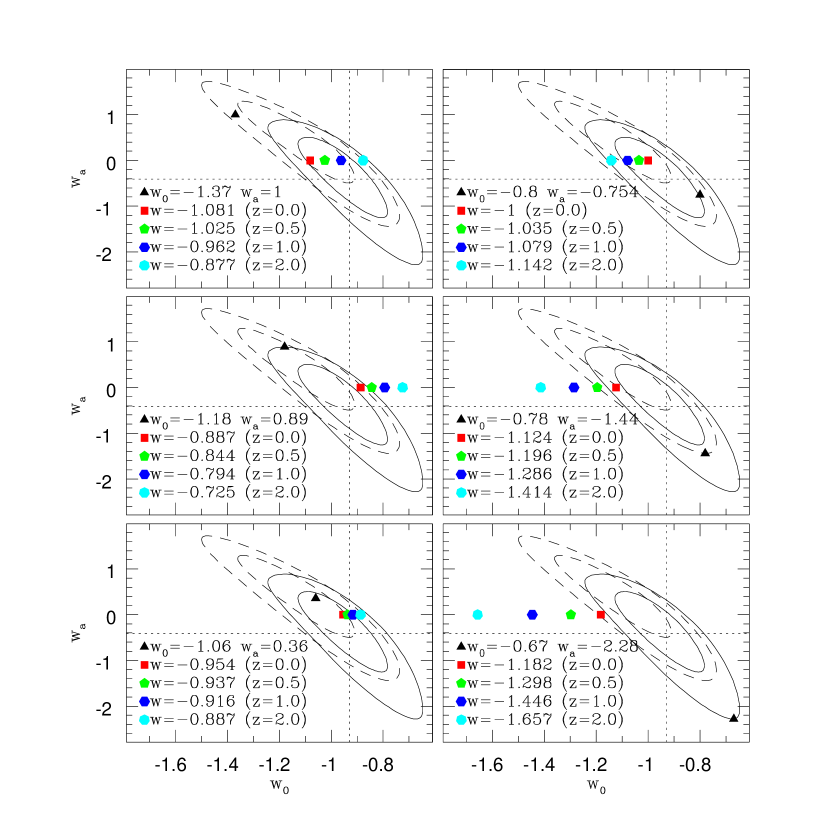
Figure 2: Each box in this Figure refers to a single $\cal A$ model (black triangle) and the related $\cal W$$(z)$ models (color polygones). Notice that, in most cases, distances between colored polygones are smaller than their distance from the black triangle. This outlines the possibility of a serious bias in data analysis, if tested by assuming constant $w$ cosmologies.

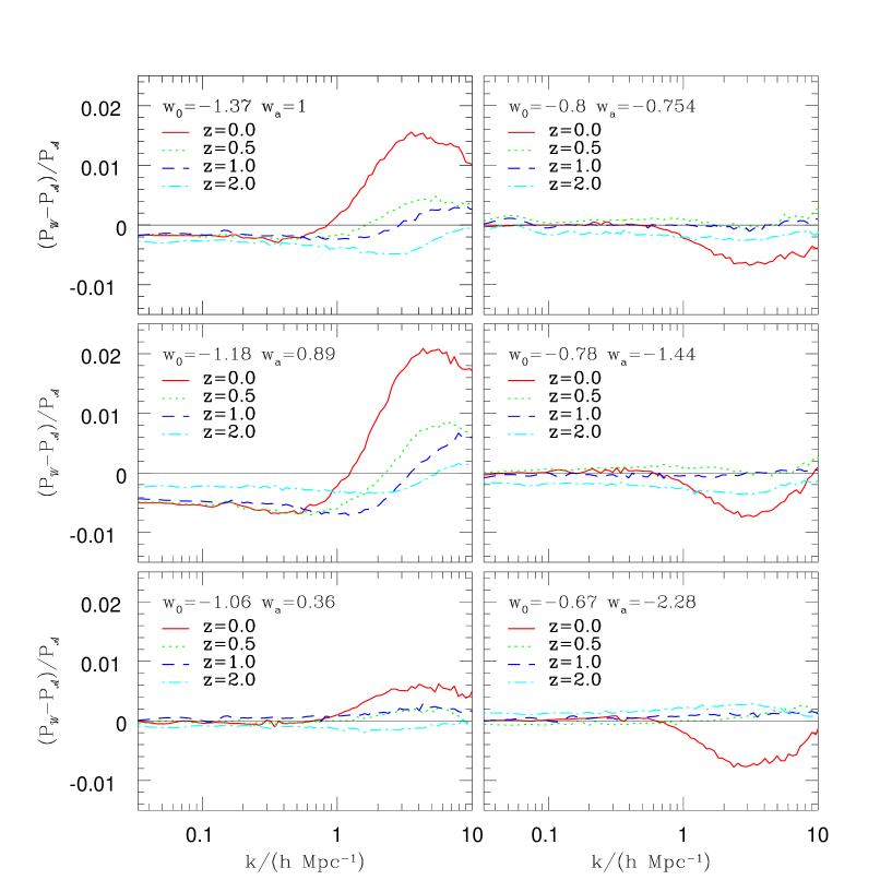
Figure 3: Spectral discrepancies at various redshift. Each box refers to a single $\cal A$ model (same ordering as in previous Figure). Discrepancies are however greatest at $z=0$ and, at such redshift only, attain $2\,\%$ in models with $w_{o}\ll-1$. The $k$ value where such large discrepancy is reached, however, is $\sim 4$–$5\,h\,$Mpc^-1, well above the $k$–range where gas dynamics can be ignored, if aiming at $\sim 1\,\%$ precision. Keeping within $k\simeq 4$–$5\,h\,$Mpc^-1, the top discrepancy is always $<1\,\%~{}.$

4 Results

In what follows, $\cal A$ models will be ordered according to increasing values of the parameter $w_{o}~{},$ from $\cal A$$1$ to $\cal A$$6$. In Figure 2 I report the setting of $\cal A$’s and related $\cal W$–models on the $w_{o}$–$w_{a}$ plane, for $z=0,~{}0.5,~{}1,~{}2~{}$.

The $\cal A$$1$ cosmology was consistent with WMAP5 and is apparently outside the 2–$\sigma$ curve for WMAP7. It should be however reminded that the significant shift of the ellipses is unlikely due to the fresh CMB inputs, while omitting to impose the distance prior [5, 6] surely had an impact on it.

Figure 2 indicates that the distance between $\cal W$ models, lying on the $w_{a}=0$ line, by definition, is mostly smaller than their distance from $\cal A$. Distances however scale with $w_{o}$ and are smaller for the central $w_{o}$ values. I shall return on this point in the next Section.

Figure 3 then shows spectral discrepancies. Within $k=3\,h\,$Mpc^-1 the maximum discrepancy is reached for $\cal A$$1$ and $\cal A$$2$ at $z=0$, attaining 1.4 and 1.6$\,\%$, respectively. Owing to [17], however, this is a scale where baryon dynamics affects spectra already more than 1–2$\,\%$. In Paper I we actually took $k=3\,h\,$Mpc^-1 as a limit; in this scale range, however, the discrepancy is rapidly bursting and, should we keep within $k=2\,h\,$Mpc^-1, no spectral discrepancy exceeds 1$\,\%$.

It is however clear that the other models exhibit a nicer behavior. Even the $\cal A$$6$ model, whose distance from $\Lambda$CDM is similar to $\cal A$$1$, exhibits discrepancies within $0.8\,\%$, up to $k=10~{}.$ Other models are even nicer, exhibiting discrepancies in the range of the permil.

Discrepancies decrease with increasing $z$ and, at $z=0.5$ are mostly in the permil range, for all models.

5 Discussion

This finding perfectly fits the reason why spectral similarities are expected. When using the conformal time $\tau$, the background cosmic metric reads $ds^{2}=a^{2}(\tau)(d\tau^{2}-d\ell^{2})$. Equal comoving distance means then that equal conformal times have elapsed. Most events, on a cosmological scale, are indeed scheduled in accordance with the conformal time $\tau~{}$; the ordinary time $t$, instead, sets a correct “timing” in virialized environments, where local minkowskian reference frames no longer feel the scale factor evolution. Accordingly, it makes sense to set aside models with equal “conformal age”, expecting increasing discrepancies when time elapses and, however, on scales virialized since longer. Up to $k\sim 2$–$3\,h\,$Mpc^-1 we are inspecting scales $>\sim L=2\pi/k\sim 2\,h^{-1}$Mpc; still at $z=0$, there are quite a few virialized systems on such scales, which however correspond to density peaks more and more above average, as we go towards higher $z~{}$.

A further comment is deserved by the proximity of auxiliary models on the $w_{o}$–$w_{a}$ plane. In quite a few cases, as for the models $\cal A$$3$ and $\cal A$$4$, they almost overlap. This envisages a danger, in future observational analysis; it is reasonable to expect that a first data test is carried by assuming constant $w$. Let us suppose, for instance, that the real cosmology is close to the model $\cal A$4. It is not unlikely that all the models indicated by colored polygones are then compatible with a single $w$ value, e.g. -1.18$\pm 0.10~{}.$

As a matter of fact, starting from the setting of each triangle, we could draw a bunch of curves, indicating the loci of equal $\tau_{o}-\tau_{rec}$ (difference between conformal present and recombination times), when $w_{a}$ varies. When these curves diverge fast enough, there is a realistic possibility that they cross the $w_{a}=0$ line on reasonably distant sites. Otherwise, the risk of spurious constant–$w$ detection is a serious danger. One should also take into account that the very assumption of a polynomial $w(a)$ is a simplifying ansatz, and that there can be cosmologies behaving even more dangerously, e.g. some cosmology arising from a tracking potential.

In this context, the very discrepancies detected above $k\sim 2$–$3\,h\,$Mpc^-1 are welcome. These scales still need to be tested through hydro simulations, but a reliable pattern for data analysis could actually start from the assumption of constant–$w$, so individuating a bunch of curves, characterized by constant $\tau_{o}-\tau_{rec}$, which will be the models among which one will discriminate through higher–$k$ spectral discrepancies.

Appendix A Reproduction of the likelihood ellipses with the Bézier curves

The algebraic technique used to reproduce the ellipses in Figure 1 is named after Bézier and is largely used in vector graphics to model smooth curves which can be scaled indefinitely, without any bound, by the limits of rasterized images. In the PostScript files in the WMAP $\Lambda$–site, I found the coefficients for the cubic Bézier curves:

$${\bf B}(u)=(1-u)^{3}{\bf P}_{0}+3(1-u)^{2}u{\bf P}_{1}+3(1-u)u^{2}{\bf P}_{2}+u^{3}{\bf P}_{3}~{}~{}u\in[0,1]$$ (3)

yielding 1– and 2–$\sigma$ contours. Here the vector B, running on the $w_{0}$–$w_{a}$ plane, describes a curve fixed by the positions of the points $P_{k}$ (k=0,…,3), when $u$ varies from 0 to 1. Further details on this technique can be found in a previous paper [19], where the coordinates of Bézier points for WMAP5 ellipses are also reported. Here below I report the coordinates of the Bézier points to draw WMAP7 ellipses.

	$x_{0}$	$y_{0}$	$x_{1}$	$y_{1}$	$x_{2}$	$y_{2}$	$x_{3}$	$y_{3}$
i
1	-1.1203	0.4568	-1.0857	0.6227	-0.9828	0.3566	-0.8997	-0.0810
2	-0.8997	-0.0810	-0.8166	-0.5186	-0.7648	-1.0959	-0.7890	-1.2234
3	-0.7890	-1.2234	-0.8132	-1.3508	-0.9069	-1.0583	-1.0034	-0.5500
4	-1.0034	-0.5500	-1.0999	-0.0416	-1.1483	0.3225	-1.1203	0.4568

	$x_{0}$	$y_{0}$	$x_{1}$	$y_{1}$	$x_{2}$	$y_{2}$	$x_{3}$	$y_{3}$
i
1	-1.2385	0.7974	-1.1949	1.0412	-1.0062	0.8187	-0.8278	-0.1565
2	-0.8278	-0.1565	-0.6626	-1.0603	-0.6270	-2.1171	-0.6565	-2.2500
3	-0.6565	-2.2500	-0.6941	-2.4197	-0.8457	-1.8601	-1.0139	-0.8592
4	-1.0139	-0.8592	-1.1822	0.1417	-1.2679	0.6336	-1.2385	0.7974

Table 1: Points defining the 4 cubic Bézier expressions yielding the 1–$\sigma$ and 2–$\sigma$ curves (upper and lower table, respectively).

References

References

- [1] Colombo L & Gervasi M, 2006 J. Cosmol. Astropart. Phys. 10 001
- [2] La Vacca G & Kristiansen J, 2009 JCAP 907036
- [3] Wetterich C, 1988 Nucl.Phys.B, 302 668
- [4] Ratra B & Peebles P.J.E., 1988 Phys.Rev.D 37 3406
- [5] Komatsu E et al., 2009 Astrophys. J. Suppl. 180 330
- [6] Komatsu E et al., arXiv:1001.4538
- [7] Manera M & Mota D, 2006 Mon. Not. R. Astron. Soc. 371 1373
- [8] Mota D, 2008 J. Cosmol. Astropart. Phys. 9 006
- [9] Refregier A et al., 2010, arXiv 1001.0061
- [10] Huterer D and Takada M, 2005 Astrophys. J. 23 369
- [11] Klypin A, Macciò A V, Mainini R and Bonometto S A, 2003 Astrophys. J. 599 31
- [12] Linder E and White M, 2005 Phys. Rev. D 72, 061394
- [13] Macciò A V, Quercellini C, Mainini R, Amendola L, Bonometto S A, 2004 Phys. Rev. D 69 123516
- [14] Solevi P, Mainini R, Bonometto S A, Macciò A V, Klypin A and Gottlöber S, 2006 Mon. Not. R. Astron. Soc. 366 1346
- [15] Francis M J, Lewis G F and Linder E V, 2007 Mon. Not. R. Astron. Soc. 380 1079
- [16] Casarini L, Macciò A V & Bonometto S A, 2009 J. Cosmol. Astropart. Phys. 3 14 (Paper I)
- [17] Casarini L, Macciò A V & Bonometto S A, 2010, arXiv:1005.4683
- [18] Stadel J G, 2001 PhD thesis University of Washington
- [19] Casarini L, 2010, New Astron. 15 575