Parameter identifiability in a class of random graph mixture models

Abstract

We prove identifiability of parameters for a broad class of random graph mixture models. These models are characterized by a partition of the set of graph nodes into latent (unobservable) groups. The connectivities between nodes are independent random variables when conditioned on the groups of the nodes being connected. In the binary random graph case, in which edges are either present or absent, these models are known as stochastic blockmodels and have been widely used in the social sciences and, more recently, in biology. Their generalizations to weighted random graphs, either in parametric or non-parametric form, are also of interest in many areas. Despite a broad range of applications, the parameter identifiability issue for such models is involved, and previously has only been touched upon in the literature. We give here a thorough investigation of this problem. Our work also has consequences for parameter estimation. In particular, the estimation procedure proposed by Frank and Harary for binary affiliation models is revisited in this article.

1 Introduction

In modern statistical analyses, data is often structured using networks. Complex networks appear across many fields of science, including biology (metabolic networks, transcriptional regulatory networks, protein-protein interaction networks), sociology (social networks of acquaintance, or other connections between individuals), communications (the Internet), and others.

The literature contains many random graph models which incorporate a variety of characteristics of real-world graphs (such as scale-free or small-world properties). We refer to Newman (2003) and the references therein for an interesting introduction to networks.

One of the earliest and most studied random graph models was formulated by Erdős and Rényi (1959). In this setup, binary random graphs are modeled as a set of independent and identically distributed Bernoulli edge variables over a fixed set of nodes. The homogeneity of this model led to the introduction of mixture versions to better capture heterogeneity in data. Stochastic blockmodels (Daudin et al., 2008; Frank and Harary, 1982; Holland et al., 1983; Snijders and Nowicki, 1997) were introduced in various forms, primarily in the social sciences (White et al., 1976) to study relational data, and more recently in biology (Picard et al., 2009). In this context, the nodes are partitioned into latent groups (blocks) characterizing the relations between nodes. Blockmodelling thus refers to the particular structure of the adjacency matrix of the graph (i.e., the matrix containing edge indicators). By ordering the nodes by the groups to which they belong, this matrix exhibits a block pattern. Diagonal and off-diagonal blocks, respectively, represent intra-group and inter-group connections. In the special case where blocks exhibit the same behavior within their type (diagonal or off-diagonal), we obtain a model with an affiliation structure (Frank and Harary, 1982).

Although the literature from the social sciences has focused mostly on binary relations, there is a growing interest in weighted graphs (Barrat et al., 2004; Newman, 2004). Mixture models have also been considered in the case of a finite number of possible relations (Nowicki and Snijders, 2001), and more recently with continuous edge variables (Ambroise and Matias, 2010; Mariadassou and Robin, 2010). Some variations that we shall not discuss here include models with covariates (Tallberg, 2005), mixed membership models (Airoldi et al., 2008; Latouche et al., 2009), and models with continuous latent variables (Daudin et al., 2010; Handcock et al., 2007). We also note that Newman and Leicht (2007) proposed another version of a binary mixture model, slightly different from the stochastic blockmodel considered here.

Many different parameter estimation procedures have been proposed for these models, such as Bayesian methods (Nowicki and Snijders, 2001; Snijders and Nowicki, 1997), variational Expectation-Maximization (EM) procedures (Daudin et al., 2008; Picard et al., 2009), online classification EM methods (Zanghi et al., 2008, 2010) and more recently, direct mixture model based approaches (Ambroise and Matias, 2010). Consistency of all these procedures relies strongly on the identifiability of the model parameters. However, the literature on these models has not addressed this question in any depth. The trivial label-swapping problem is often mentioned: it is well known that the parameters may be recovered only up to permutations on the latent class labels. Whether this is the only issue preventing unique identification of parameters from the distribution, however, has never been investigated. Given the complex form of the model parameterization, this is not surprising, as any such analysis seems likely to be very involved.

In earlier work, (Allman et al., 2009, Theorem 7), the authors made a first step towards an understanding of the parameter identifiability issue in binary random graph mixture models. While that article addressed a variety of models with latent variables, the present one focuses more specifically on random graph mixtures, giving parameter identifiability results for a broad range of such models. Moreover, part of our work sheds some new light on parameter estimation procedures.

Allman et al. (2009) emphasized the usefulness of an algebraic theorem due to Kruskal (1976, 1977) (see also Rhodes, 2010) to establish identifiability results in various models whose common feature is the presence of latent groups and at least three conditionally independent variables. Here, we rather focus on the family of random graph mixture models and explore various techniques to establish their parameters’ identifiability. Thus while the method developed by Allman et al. (2009) is presented in Section 5.1 and finds further use in several arguments, it is only one of several techniques we use. The issue at the core of Kruskal’s result is the decomposition of a 3-way array as a sum of rank one tensors. While there exist approximate methods of performing this decomposition (see, e.g., Tomasi and Bro, 2006), we mention that this approach seems poorly-suited to explicitly recover the parameters from the distribution, and thus to construct estimation procedures.

Some of our results focus on moment equations, as did those of Frank and Harary (1982), in one of the earliest works on binary affiliation models. In particular, we revisit some of their claims. The method consists in looking at the distribution of $K_{n}$, a complete set of edge variables over a set of $n$ nodes. A natural question is then: What is the minimal value of $n$ such that the complete distribution over all edge variables (a potentially infinite set) is characterized by the distribution of $K_{n}$? Despite this question’s simplicity, we are far from having a complete answer to it. When looking at finite state distributions (e.g., for binary random graphs), the knowledge of the distribution of $K_{n}$ is equivalent to the knowledge of a certain set of moments of the distribution. Expressing the moments in terms of parameters gives a nonlinear polynomial system of equations, which one uses to identify parameters. The uniqueness of solutions to those systems, up to label swapping on parameters, is the issue at stake for identifiability.

For random graphs with continuous edge weights given by a parametric family of distributions we shall see that the information contained in the model might be recovered from the distribution of $K_{n}$ for very small values of $n$. In this case, we rely on classical results on the identifiability of the parameters of a multivariate mixture due to Teicher (1967). Note that the main difference between classical mixtures and random graph mixtures is the non-independence of the variates.

In contrast to the approach based on Kruskal’s Theorem, both the method utilizing moment equations and the one relying on multivariate mixtures lead to practical estimation procedures. These are further developed by Ambroise and Matias (2010).

In Allman et al. (2009), a large role was played by the notion of generic identifiability, by which every parameter except those lying on a proper algebraic subvariety, are identifiable. In other words, in a parametric setting, the non-identifiable parameters are included in a subset whose dimension is strictly smaller than the dimension of the full parameter space. Thus with probability one with respect to the Lebesgue measure, every parameter is identifiable. This notion of generic identifiability is important for finite mixtures of multivariate Bernoulli distributions (Allman et al., 2009; Carreira-Perpiñán and Renals, 2000; Gyllenberg et al., 1994) and also for hidden Markov models (Allman et al., 2009; Petrie, 1969). Here, we stress that some of our identifiability results are generic, while others are strict.

Finally, we note that our focus throughout will be on undirected graph models. While many of our results may be generalized to directed graphs, one must pay careful attention to the models’ parametrization in doing so. For instance, some of the results would become simpler if the connectivities from group $q$ to group $l$ differed from those from group $l$ to group $q$, as symmetry in a model can have a strong impact on identifiability questions. However, such asymmetric models require an increase in the number of parameters which may be excessive for data analysis.

This paper is organized as follows. Section 2 presents the various random graph mixture models: with either binary or, more generally, finite-state edges; both parametric and non-parametric models for edges with continuous weights; and the particular affiliation variant of these models. Section 3 gives parameter identifiability results for binary random graphs. Note that the affiliation model has to be handled separately. Section 4 takes up weighted random graphs, in both parametric and non-parametric variants. All the proofs are postponed to Section 5. In particular, Section 5.1 is devoted to a brief presentation of Kruskal’s result and our use of it in the proofs of Theorems 2 and 14.

2 Notation and models

We consider a probabilistic model on undirected and possibly weighted graphs as follows. Let $n$ be a fixed number of nodes, with $Z_{1},\ldots,Z_{n}$ independent identically distributed (i.i.d.) random variables, taking values in $\mathcal{Z}=\{1,\ldots,Q\}$ for some $Q\geq 2$. These random variables represent the $Q$ groups the nodes are partitioned among, and are used to introduce heterogeneity in the model. With $\pi_{q}=\mathbb{P}(Z_{i}=q)\in(0,1)$, so $\sum_{q}\pi_{q}=1$, the vector $\boldsymbol{\pi}=(\pi_{q})$ thus gives the priors on the groups. Let $\{X_{ij}\}_{1\leq i<j\leq n}$ be random edge variables taking values in a state space $\mathcal{X}$. Conditional on $Z_{1},\ldots,Z_{n}$, we assume that the edge variables $\{X_{ij}\}_{1\leq i<j\leq n}$ are independent, and that the conditional distribution of $X_{ij}$ depends only on $Z_{i}$ and $Z_{j}$, the groups containing its endpoints.

We are interested in random graphs of various types: For binary random graphs, where $\mathcal{X}=\{0,1\}$, an absent edge is represented by $0$ and a present one by $1$. Random graphs whose edges may be of finitely many types are modeled with $\mathcal{X}=\{1,\ldots,\kappa\}$, or equivalently, $\{0,\ldots,\kappa-1\}$. More general weighted random graphs are obtained when $\mathcal{X}=\mathbb{N}$ or $\mathbb{R}^{s},s\geq 1$.

In the binary state case, the distribution of $X_{ij}$ conditional on $Z_{i},Z_{j}$ follows a Bernoulli distribution with parameter $p_{Z_{i}Z_{j}}=\mathbb{P}(X_{ij}=1|Z_{i},Z_{j})$. As we consider only undirected graphs, we implicitly assume equality of the parameters $p_{ql}=p_{lq}$, for all $1\leq q,l\leq Q$.

More generally, in the finite state case, with $\mathcal{X}=\{1,\ldots,\kappa\}$, the vector $\mathbf{p}_{Z_{i}Z_{j}}=(p_{Z_{i}Z_{j}}(1),\ldots,p_{Z_{i}Z_{j}}(\kappa))$ contains the values $p_{Z_{i}Z_{j}}(k)=\mathbb{P}(X_{ij}=k|Z_{i},Z_{j})$, for $1\leq k\leq\kappa$, with $\sum_{k}p_{Z_{i}Z_{j}}(k)=1$. We also implicitly assume equality of the vectors $\mathbf{p}_{ql}=\mathbf{p}_{lq}$, for all $1\leq q,l\leq Q$. We introduce this model primarily as a tool in the study of continuously weighted random graphs, though it might be useful for studying relationships between nodes of different types (colors), or of varying but discrete strengths (viewing the states as ordered). Note that a related model is described by Nowicki and Snijders (2001), where the authors consider more general relation types (not necessarily edges, whether directed or not) occurring between a pair of nodes.

In the weighted random graph case, edges may be viewed as either absent ($X_{ij}=0$) or present ($X_{ij}\neq 0$), with those present having a weight, namely a non-zero value in $\mathcal{X}=\mathbb{N}$, $\mathbb{R}$, or $\mathbb{R}^{s}$. The distribution of $X_{ij}$ conditional on $Z_{i},Z_{j}$ may be assumed to have either a parametric or non-parametric form. More precisely, we assume that the distribution of $X_{ij}$ conditional on $Z_{i},Z_{j}$ is the probability measure $\mu_{Z_{i},Z_{j}}$ on $\mathcal{X}$ given by

$$\mu_{ql}=(1-p_{ql})\delta_{0}+p_{ql}F_{ql},\quad 1\leq q,l\leq Q,$$

where $p_{ql}\in(0,1]$ is a sparsity parameter, $\delta_{0}$ is the Dirac mass at zero and $F_{ql}$ is a probability measure on $\mathcal{X}$ with density $f_{ql}$ with respect to either the counting measure on $\mathbb{N}$ or the Lebesgue measure on $\mathbb{R}$ or $\mathbb{R}^{s}$. We also implicitly assume $\mu_{ql}=\mu_{lq}$, for all $1\leq q,l\leq Q$. In the parametric case, we assume moreover that $F_{ql}=F(\cdot,\theta_{ql})$ and $f_{ql}=f(\cdot,\theta_{ql})$ where the parameter $\theta_{ql}$ belongs to $\Theta\subset\mathbb{R}^{p}$. In the non-parametric case we assume $F_{ql}$ is absolutely continuous.

We shall always assume that $F_{ql}$ has no point mass at zero, otherwise the sparsity parameter $p_{ql}$ cannot be identified from the mixture $\mu_{ql}$. For instance, when considering Poisson weights, $f_{ql}$ is the Poisson density truncated at zero,

$$f_{ql}(k)=\frac{\theta_{ql}^{k}}{k!}(e^{\theta_{ql}}-1)^{-1},\quad k\geq 1.$$

A particular instance of these models is the affiliation one, which assumes additionally only two distributions of connections between the edges, one for intra-group connections and another for inter-group connections. Thus the binary state case of the affiliation model assumes

$$p_{ql}=\begin{cases}\alpha&\text{ if }q=l,\\ \beta&\text{ if }q\neq l,\end{cases}\quad\text{ for all }q,l\in\{1,\ldots,Q\}.$$

The affiliation model in the continuous observations case is described similarly with $\mu_{ql}=\mu_{\text{in}}1_{q=l}+\mu_{\text{out}}1_{q\neq l}$, for all $1\leq q,l\leq Q$. More precisely, in the continuous parametric case, for all $q,l\in\{1,\ldots,Q\}$ we set

$$p_{ql}=\begin{cases}\alpha&\text{ if }q=l,\\ \beta&\text{ if }q\neq l,\end{cases}\quad\text{ and }\quad\theta_{ql}=\begin{cases}\theta_{\text{in}}&\text{ if }q=l,\\ \theta_{\text{out}}&\text{ if }q\neq l.\end{cases}$$

For all these models, we consider restrictions of the model distribution by focusing on a subset of the nodes. We denote by $K_{n}$ the complete set of $\binom{n}{2}$ edge variables associated to a subset of $n$ nodes. Note that the distribution of these variables is independent of the choice of which $n$ nodes one considers. Also, while this notation is motivated by that used in graph theory, where $K_{n}$ denotes the complete graph on $n$ nodes, we emphasize that here $K_{n}$ is a set of random variables, and we are making no statement as to whether these edges are present or absent in any realization of our model.

3 Binary random graphs

We first focus on models with binary edge states, considering the more general case with arbitrary connectivity parameters, followed by affiliation models.

3.1 The non-affiliation case

When $\mathcal{X}=\{0,1\}$, a first result on identifiability of parameters was obtained by Allman et al. (2009) for the special case of $Q=2$ groups. For completeness, we recall the statement here.

Theorem 1.

(Allman et al., 2009, Theorem 7). The parameters $\pi_{1},\pi_{2}=1-\pi_{1},p_{11},p_{12},p_{22}$ of the random graph mixture model with binary edge state variables and $Q=2$ groups are identifiable, up to label swapping, from the distribution of $K_{16}$ provided that the connectivity parameters $\{p_{11},p_{12},p_{22}\}$ are distinct.

In particular, the result remains valid when the group proportions $\pi_{q}$ are fixed.

Note the assumption that $p_{11}\neq p_{22}$ limits this theorem to the strict non-affiliation case.

The proof of this theorem is based on a clever application of an algebraic result, due to Kruskal (1976, 1977) (see also Rhodes, 2010), that deals with decompositions of 3-way arrays. While generalizing the proof to more than two groups requires substantially more effort, the basic method still applies. Here we prove the following theorem.

Theorem 2.

The parameters $\pi_{q}$, $1\leq q\leq Q$, and $p_{ql}=\mathbb{P}(X_{ij}=1|Z_{i}=q,Z_{j}=l)$, $1\leq q\leq l\leq Q$, of the random graph mixture model with binary edge state variables and $Q\geq 3$ groups are generically identifiable, up to label swapping, from the distribution of $K_{m^{2}}$, when

$$\left\{\begin{array}[]{ll}m\geq Q-1+(Q+2)^{2}/4&\text{ if }Q\text{ is even},\\ m\geq Q-1+(Q+1)(Q+3)/4&\text{ if }Q\text{ is odd}.\end{array}\right.$$

Moreover, the result remains valid when the group proportions $\pi_{q}$ are fixed.

Note that the stated number of nodes ensuring that parameters are generically identifiable from the distribution of the edges may not be optimal. In particular, when $Q=2$, the proof of this theorem is still valid, yet it gives a minimal number of $m^{2}=25$ nodes. This is larger than the bound $16$ obtained in Theorem 1, and that number may itself not be optimal.

Also, while Theorem 1 gives exact restrictions on parameters producing identifiability, Theorem 2 is not explicit about the generic conditions. However, for any fixed $Q$ the argument in our proof does yield a straightforward, though perhaps lengthy, means of checking whether a particular choice of parameters meets the conditions. Among these is a requirement that the $p_{ql}$ be distinct, so the theorem does not apply to the affiliation model.

Moreover, a careful reading of the proof of the theorem shows that its generic aspect concerns only the part of the parameter space with the connectivities $p_{ql}$. This enables us to conclude that even when considering subsets defined by restriction of the group proportions $\pi_{q}$ (for instance assuming the group proportions are fixed, or equal), the result remains valid.

3.2 The affiliation model

In the particular case of the affiliation model, we can obtain results from arguments based on moments of the distribution. For a small number of nodes, one may obtain explicit formulas for the moments in terms of model parameters. By analyzing the solutions to this nonlinear multivariate polynomial system of equations, one can address the question of parameter identifiability, as well as develop estimation procedures.

3.2.1 Relying on the distribution of $K_{3}$.

Frank and Harary (1982) presented a method for estimation of the parameters of the binary affiliation model based only on the distribution of triplet cycles $(X_{ij},X_{jk},X_{ki})$, $1\leq i<j<k\leq n$, of edge variables. From an identifiability perspective, this corresponds to identifying the parameters from the distribution of $K_{3}$. They suggest estimation of the parameters by solving the empirical moment equations. However, they omit discussing uniqueness of the solutions to these equations, even though this issue is a delicate one for nonlinear equations.

In the following, we first explore the use of the distribution of only $K_{3}$ to identify model parameters. As a consequence, we exhibit a new estimation procedure for the parameters.

The distribution of a triplet $(X_{ij},X_{jk},X_{ki})$, is expressible in terms of the indeterminates $\alpha,\beta$ and $\pi_{q}$s. Let us denote by $s_{2}$ and $s_{3}$ the sums of the squares and cubes of the $\pi_{q}$s and, more generally, let

$$s_{k}=\sum_{q=1}^{Q}\pi_{q}^{k}.$$

Then one easily computes (see also Frank and Harary, 1982) the moment formulas

$$m_{1} = \mathbb{E}(X_{ij})=s_{2}\alpha+(1-s_{2})\beta,$$ (1)

$$m_{2} = \mathbb{E}(X_{ij}X_{ik})=s_{3}\alpha^{2}+2(s_{2}-s_{3})\alpha\beta+(1-2s_{2}+s_{3})\beta^{2},$$ (2)

$$m_{3} = \mathbb{E}(X_{ij}X_{ik}X_{jk})=s_{3}\alpha^{3}+3(s_{2}-s_{3})\alpha\beta^{2}+(1-3s_{2}+2s_{3})\beta^{3},$$ (3)

which completely characterize the distribution of $(X_{ij},$ $X_{jk},X_{ki})$.

Note that in the important case of a uniform node distribution, where $\pi_{q}=1/Q$ for all $q$, we have $s_{k}=Q^{1-k}$. This implies $s_{3}=s_{2}^{2}$, and hence $m_{2}=m_{1}^{2}$, so these equations reduce to two independent ones. As a consequence, the claim by Frank and Harary (1982) that it is then possible to estimate the three unknowns $Q,\alpha,\beta$ relying only on these moment equations is not correct.

Still, there are indeed several situations in which parameters are identifiable from these moments, as we next discuss.

With $Q=2$ latent groups and a possibly non-uniform group distribution, there are 3 independent parameters in the affiliation model. In this case, the three moments above are enough to identify parameters. To show this, we first construct certain polynomials with roots at the connectivity parameters. Since the construction easily extends to larger $Q$, we give it more generally.

Proposition 3.

Consider the random graph affiliation mixture model with $Q\geq 2$ groups and binary edge state variables, on $Q+1$ nodes. Then the parameter $\alpha$ is a real root of the degree $\binom{Q+1}{2}$ univariate polynomial

$$U_{Q}(X)=\mathbb{E}\left(\prod_{1\leq i<j\leq Q+1}(X-X_{ij})\right).$$

The polynomial

$$V_{Q}(X,Y)=\mathbb{E}\Big{(}\Big{(}X+(Q-1)Y-\sum_{1\leq i\leq Q}X_{i(Q+1)}\Big{)}\prod_{1\leq i<j\leq Q}(X-X_{ij})\Big{)}$$

of degree $\binom{Q}{2}+1$ in $X,$ and degree 1 in $Y,$ vanishes at $(X,Y)=(\alpha,\beta)$. Moreover, the coefficient of $Y$ in $V_{Q}(\alpha,Y)$ is non-zero precisely when $\alpha\neq\beta$.

The utility of these polynomials is that from the distribution of $K_{Q+1}$, the polynomial $U_{Q}$ allows one to recover at most $\binom{Q+1}{2}$ candidate values for $\alpha$, and then for each such value $V_{Q}$ allows one to recover a unique candidate for $\beta$. While some of these candidates could be ruled out as not lying in $(0,1)$, we do not know when this leaves a unique $\alpha$ and $\beta$ for $Q\geq 3$. In the case of $Q=2$ groups, however, we prove that these polynomials uniquely identify the parameters.

Theorem 4.

In the random graph affiliation mixture model with $Q=2$ groups and binary edge state variables, the parameter $\alpha$ is the unique real root of the polynomial

$$U_{2}(X)=X^{3}-3m_{1}X^{2}+3m_{2}X-m_{3}.$$

Moreover, as soon as $\alpha\neq\beta$, the parameter $\beta$ is the unique real root of the polynomial $V_{2}(\alpha,Y)$ where

$$V_{2}(X,Y)=X^{2}+XY-3m_{1}X-m_{1}Y+2m_{2}.$$

Once $\alpha$ and $\beta$ are uniquely identified, we may determine from equation (1) the value of $s_{2}$ (again using that $\alpha\neq\beta$), and hence $\pi_{1}$, $\pi_{2}$, up to permutation. This proves the following corollary.

Corollary 5.

The parameters $\{\pi_{1},\pi_{2}=1-\pi_{1}\}$, up to label swapping, and $\alpha,\beta$ of the random graph affiliation mixture model with $Q=2$ groups and binary edge state variables are strictly identifiable from the distribution of $K_{3}$ provided $\alpha\neq\beta$.

Identifiability of $\alpha$ and $\beta$ when $Q$ and the $\pi_{q}$s are known

When the $\pi_{q}$s are known, Frank and Harary (1982) suggested solving any two of the three empirical counterparts of equations (1), (2) and (3), leading to three different methods of estimating $\alpha$ and $\beta$. However, numerical experiments convinced us that two equations are in general not sufficient to uniquely determine the parameters. In fact, it is not immediately clear that even with the three moment equations (either the theoretical ones for the question of identification, or their empirical counterparts for estimation) a unique solution is determined. Below we give explicit formulas for the solution to the system, which in most cases are even rational, involving no extraction of roots. These can thus be easily used to construct estimators.

Theorem 6.

If $m_{2}\neq m_{1}^{2}$, then $\boldsymbol{\pi}$ is non-uniform and we can recover the parameters $\beta$ and $\alpha$ via the rational formulas

$$\beta = \frac{(s_{3}-s_{2}s_{3})m_{1}^{3}+(s_{2}^{3}-s_{3})m_{2}m_{1}+(s_{3}s_{2}-s_{2}^{3})m_{3}}{(m_{1}^{2}-m_{2})(2s_{2}^{3}-3s_{3}s_{2}+s_{3})},$$

$$\alpha = \frac{m_{1}+(s_{2}-1)\beta}{s_{2}}.$$

If $m_{2}=m_{1}^{2}$, then $\boldsymbol{\pi}$ is uniform and we have

$$\beta=m_{1}+\left(\frac{m_{1}^{3}-m_{3}}{Q-1}\right)^{1/3}\quad\text{and}\quad\alpha=Qm_{1}+(1-Q)\beta.$$

Implicit in this statement is the fact that denominators in the above formulas are non-zero. Note that the uniform group prior case formula is used for estimation by Ambroise and Matias (2010).

We immediately obtain the following corollary.

Corollary 7.

For any fixed and known values of $\pi_{q}\in(0,1)$, $1\leq q\leq Q$, both parameters $\alpha,\beta$ of the random graph affiliation model with binary edge state variables are identifiable from the distribution of $K_{3}$.

The proofs of the previous statements lead to an interesting polynomial in the moments, whose vanishing detects the Erdős-Rényi model, corresponding to a single node group.

Proposition 8.

The moments of a random graph affiliation model with binary edge state variables, $Q$ node states, and $\alpha\neq\beta$ satisfy

$$2m_{1}^{3}-3m_{1}m_{2}+m_{3}=0$$

if, and only if, $Q=1$.

This proposition follows from expressing the moments in terms of parameters to see that

$$2m_{1}^{3}-3m_{1}m_{2}+m_{3}=(\alpha-\beta)^{3}(2s_{2}^{3}-3s_{2}s_{3}+s_{3}),$$

together with the determination in the proof of Lemma 19 in Section 5.3 that $2s_{2}^{3}-3s_{2}s_{3}+s_{3}\neq 0$ when $\pi_{q}>0$ for more than one group $q$.

3.2.2 Relying on the distribution of $K_{4}$

We next investigate parameter identifiability from the distribution of the edge variables over more than $3$ nodes, paying particular attention to the case of $n=4$ nodes.

Necessary conditions for identifiability of the $\pi_{q}$s, when $Q$ is known

First, we establish that for an affiliation model, if the $\pi_{q}$s are unknown and are to be recovered from the distribution of $K_{n}$, then one must look at at least $n=Q$ nodes. Note that this applies not only to the binary edge state model, but to more general weighted edge models as well.

Proposition 9.

In order to identify, up to label swapping, the parameters $\{\pi_{q}\}_{1\leq q\leq Q}$ from an affiliation random graph mixture distribution on $K_{n}$ (either binary or weighted), it is necessary that $n\geq Q$.

The condition in this lemma is in general not sufficient to identify the $\pi_{q}$. Indeed, the binary edge state affiliation model with $Q=3$ has $4$ parameters. However, the set of distributions over $K_{3}$ has dimension at most $3$ (according to equations (1),(2) and (3)), which is not sufficient to identify the $4$ parameters.

Distribution on $K_{4}$

The moment formulas describing the distribution of the affiliation random graph mixture model on $K_{4}$ are given in Table 1. Note that $m_{31}$ is the same as $m_{3}$ in the last subsection, and that we omit $\mathbb{E}(X_{12}X_{34})=(\mathbb{E}(X_{12}))^{2}$ since edge variables with no endpoints in common are independent. To facilitate understanding of the moments in the table, their corresponding induced motifs are shown in Figure 1.

$m_{1}$	$\mathbb{E}(X_{12})$	$s_{2}\alpha+(1-s_{2})\beta$
$m_{2}$	$\mathbb{E}(X_{12}X_{13})$	$s_{3}\alpha^{2}+2\alpha\beta(s_{2}-s_{3})+(1-2s_{2}+s_{3})\beta^{2}$
$m_{31}$	$\mathbb{E}(X_{12}X_{13}X_{23})$	$s_{3}\alpha^{3}+3(s_{2}-s_{3})\alpha\beta^{2}+(1-3s_{2}+2s_{3})\beta^{3}$
$m_{32}$	$\mathbb{E}(X_{12}X_{13}X_{14})$	$s_{4}\alpha^{3}+3(s_{3}-s_{4})\alpha^{2}\beta+3(s_{2}-2s_{3}+s_{4})\alpha\beta^{2}$
		$+(1-3s_{2}+3s_{3}-s_{4})\beta^{3}$
$m_{33}$	$\mathbb{E}(X_{12}X_{23}X_{34})$	$s_{4}\alpha^{3}+(s_{2}^{2}+2s_{3}-3s_{4})\alpha^{2}\beta+(3s_{2}-2s_{2}^{2}-4s_{3}+3s_{4})\alpha\beta^{2}$
		$+(1-3s_{2}+s_{2}^{2}+2s_{3}-s_{4})\beta^{3}$
$m_{41}$	$\mathbb{E}(X_{12}X_{23}$	$s_{4}\alpha^{4}+2(s_{2}^{2}+2s_{3}-3s_{4})\alpha^{2}\beta^{2}+4(s_{2}-s_{2}^{2}-2s_{3}+2s_{4})\alpha\beta^{3}$
	$X_{34}X_{41})$	$+(1-4s_{2}+2s_{2}^{2}+4s_{3}-3s_{4})\beta^{4}$
$m_{42}$	$\mathbb{E}(X_{12}X_{13}$	$s_{4}\alpha^{4}+(s_{3}-s_{4})\alpha^{3}\beta+(s_{2}^{2}+2s_{3}-3s_{4})\alpha^{2}\beta^{2}$
	$X_{14}X_{23})$	$+(4s_{2}-2s_{2}^{2}-7s_{3}+5s_{4})\alpha\beta^{3}+(1-4s_{2}+s_{2}^{2}+4s_{3}-2s_{4})\beta^{4}$
$m_{5}$	$\mathbb{E}(X_{12}X_{23}X_{34}$	$s_{4}\alpha^{5}+2(s_{3}-s_{4})\alpha^{3}\beta^{2}+(2s_{3}-4s_{4}+2s_{2}^{2})\alpha^{2}\beta^{3}$
	$X_{41}X_{13})$	$+(5s_{2}-4s_{2}^{2}-10s_{3}+9s_{4})\alpha\beta^{4}+(1-5s_{2}+2s_{2}^{2}+6s_{3}-4s_{4})\beta^{5}$
$m_{6}$	$\mathbb{E}(X_{12}X_{23}X_{34}$	$s_{4}\alpha^{6}+4(s_{3}-s_{4})\alpha^{3}\beta^{3}+3(s_{2}^{2}-s_{4})\alpha^{2}\beta^{4}$
	$X_{41}X_{13}X_{24})$	$+6(s_{2}-s_{2}^{2}-2s_{3}+2s_{4})\alpha\beta^{5}+(1-6s_{2}+8s_{3}-6s_{4}+3s_{2}^{2})\beta^{6}$

Table 1: Moment formulas describing the distribution of $K_{4}$, the complete graph on $4$ nodes, for the binary affiliation model.

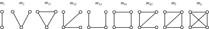
Figure 1: Correspondence between moments and motifs for $K_{4}$.

With $Q$ arbitrary, but a uniform prior on the nodes ($\pi_{q}=1/Q$, so $s_{i}=Q^{1-i}$), there are algebraic relationships between the moments on $K_{4}$, including

$$m_{2}=m_{1}^{2},\ \ m_{32}=m_{33}=m_{1}^{3},\ \ m_{42}=m_{1}m_{31},$$

and more complicated ones that can be computed using Gröbner basis methods to eliminate $\alpha$, $\beta$, and $1/Q$ from the equations. (Cox et al., 1997, provide an excellent grounding on this computational algebra.) However, the $3$ parameters $\alpha$, $\beta$, $Q$ of this affiliation model are, in fact, identifiable. Indeed such calculations show that the formulas for $m_{1}$, $m_{31}$, and $m_{41}$ alone imply the following.

Proposition 10.

The number of node groups, $Q$, in a random graph affiliation model with binary edge state variables and uniform group priors can be identified from the moments $m_{1}$, $m_{31}$, and $m_{41}$ by

$$Q=\frac{-m_{31}^{4}-m_{41}^{3}-3m_{41}m_{1}^{8}+3m_{41}^{2}m_{1}^{4}-6m_{1}^{6}m_{31}^{2}+4m_{1}^{9}m_{31}+4m_{1}^{3}m_{31}^{3}}{(m_{1}^{4}-m_{41})^{3}}.$$

Note that, replacing the moments with empirical estimators, this formula could be used for estimation of $Q$.

Of course once the formula in Proposition 10 is given, it can be most easily verified by expressing the moments in terms of parameters, and simplifying. Note that the denominator here does not vanish, as may be seen in two different ways: either by Lemma 20 in Section 5.3, or by checking that that

$$m_{41}-m_{1}^{4}=(\alpha-\beta)^{4}\frac{(Q-1)}{Q^{4}}\neq 0.$$

Once $Q$ is identified by this formula, since we are assuming $\pi_{q}=1/Q$, Corollary 7 applies so that $\alpha$ and $\beta$ are identifiable as well. Thus we have shown the following.

Corollary 11.

The parameters $\alpha$, $\beta$, and $Q$ of the random graph affiliation mixture model with binary edge state variables and uniform groups priors ($\pi_{q}=1/Q$) are identifiable from the distribution of $K_{4}$.

4 Weighted random graphs

4.1 The parametric case

In the parametric case, where $F_{ql}$ has parametric form $F(\cdot,\theta_{ql})$, we can uniquely identify the connectivity parameters under very general conditions by considering the distribution of $K_{3}$ only. Indeed, each triplet $(X_{ij},X_{ik},X_{jk})$ follows a mixture of $Q^{3}$ distributions, each with three variates, comprising

• $Q$ terms of the form $\mu_{qq}(X_{ij})\mu_{qq}(X_{ik})\mu_{qq}(X_{jk})$, each with prior $\pi_{q}^{3}$, where $1\leq q\leq Q$,

• $3Q(Q-1)$ terms of the form $\mu_{qq}(X_{ij})\mu_{ql}(X_{ik})\mu_{ql}(X_{jk})$ (permuting $i,j$ and $k$), each with prior $\pi_{q}^{2}\pi_{l}$, with distinct $q,l\in\{1,2,\ldots,Q\}$,

• $Q(Q-1)(Q-2)$ terms of the form $\mu_{ql}(X_{ij})\mu_{qm}(X_{ik})\mu_{lm}(X_{jk})$, each with prior $\pi_{q}\pi_{l}\pi_{m}$, with distinct $q,l,m\in\{1,2,\ldots,Q\}$.

By an old result due to Teicher (1967), the identifiability of finite mixtures of some family of distributions is equivalent to identifiability of finite mixtures of (multivariate) product distributions from this same family. In addition, identifiability of continuous univariate parametric mixtures is generally well understood (Teicher, 1961, 1963). Thus, we introduce the following assumptions.

Assumption 1.

The $Q(Q+1)/2$ parameter values $\theta_{ql}$, $1\leq q\leq l\leq Q$ are distinct.

Assumption 2.

The family of measures $\mathcal{M}=\{F(\cdot,\theta)~{}|~{}\theta\in\Theta\}$ satisfies

1. all elements $F(\cdot,\theta)$ have no point mass at $0$,

2. the parameters of finite mixtures of measures in $\mathcal{M}$ are identifiable, up to label swapping. In other words, for any integer $m\geq 1$,

   $$\text{if }\quad\sum_{i=1}^{m}\alpha_{i}F(\cdot,\theta_{i})=\sum_{i=1}^{m}\alpha_{i}^{\prime}F(\cdot,\theta_{i}^{\prime})\quad\text{ then }\quad\sum_{i=1}^{m}\alpha_{i}\delta_{\theta_{i}}=\sum_{i=1}^{m}\alpha_{i}^{\prime}\delta_{\theta_{i}^{\prime}},$$

   where $\delta_{\theta}$ denotes the Dirac mass at $\theta$.

Remark.

Note that most of the classical parametric families satisfy this assumption. In particular, the truncated Poisson, Gaussian and Laplace families $\{f(\cdot,\theta),\theta\in\mathbb{R}^{p}\}$ satisfy Assumption 2 (see e.g., McLachlan and Peel, 2000; Teicher, 1961, 1963).

Theorem 12.

Under Assumptions 1 and 2, the parameters $\boldsymbol{\pi}$, $\theta_{ql}$, $p_{ql}$, $1\leq q\leq l\leq Q$ of the parametric random graph mixture model with weighted edge variables are identifiable, up to label swapping, from the distribution of $K_{3}$.

The previous result is not applicable to the parametric affiliation model, for which the set $\{\theta_{ql},1\leq q\leq l\leq Q\}$ reduces to $\{\theta_{\text{in}},\theta_{\text{out}}\}$, so Assumption 1 is violated. However, in this case a similar argument again yields a full identifiability result. As suggested by Proposition 9, we use $Q$ nodes to identify the group priors.

Theorem 13.

Under Assumption 2, the parameters $\alpha,\beta,\theta_{\text{in}},\theta_{\text{out}}$ of the parametric affiliation random graph mixture model with weighted edge variables are strictly identifiable from the distribution of $K_{3}$ provided $\theta_{\text{in}}\neq\theta_{\text{out}}$. Once these have been identified, the group priors $\boldsymbol{\pi}$ can further be identified, up to label swapping, from the distribution of $K_{Q}$.

A similar approach to that of this theorem has been successfully used by Ambroise and Matias (2010) to estimate the parameters of these models. They first estimated the sparsity parameters from the induced binary edge state model, but a procedure based on the preceding theorems would not require that these be distinct.

We turn next to models with a finite number, $\kappa$, of edge weights. Our primary reason for investigating such models is the role they play in our analysis of models with non-parametric conditional distributions of edge weights, in Section 4.2. Thus we limit our investigation to the single result we need there.

Theorem 14.

The parameters of the random graph mixture model, with $\kappa$-state edge variables and $Q\geq 2$ latent groups, are identifiable, up to label swapping, from the distribution of $K_{9}$, provided $\kappa\geq\binom{Q+1}{2}$ and the $\kappa$-entry vectors $\{\mathbf{p}_{ql}\}_{1\leq q\leq l\leq Q}$ are linearly independent.

Note that the condition given here on the number of edge states is likely far from optimal. In case $Q=2$ the condition requires at least $\kappa=3$ edge states whereas we know from Theorem 1 that the parameters are identifiable for this $Q$ with only $\kappa=2$ edge states.

4.2 The non-parametric case

In the most general case of non-parametric distributions, our arguments for identifiability depend on binning the values of the edge variables into a finite set. We then apply Theorem 14 to this discretization, to obtain the following.

Theorem 15.

The parameters $\{\pi_{q},\mu_{ql}=(1-p_{ql})\delta_{0}+p_{ql}F_{ql}:1\leq q,l\leq Q\}$ of the random graph weighted non-parametric mixture model are identifiable, up to label swapping, from the distribution of $K_{9}$ provided the measures $\mu_{ql},1\leq q\leq l\leq Q$ are linearly independent.

5 Proofs

5.1 Method of proofs based on Kruskal’s theorem

In this section we review Kruskal’s theorem and describe our technique for employing it in the proofs of Theorems 2 and 14.

Kruskal’s result

We first present Kruskal’s result in a statistical context. Consider a latent random variable $V$ with state space $\{1,\ldots,r\}$ and distribution given by the column vector $\mathbf{v}=(v_{1},\ldots,v_{r})$. Assume that there are three observable random variables $U_{j}$ for $j=1,2,3$, each with finite state space $\{1,\ldots,\kappa_{j}\}$. The $U_{j}$s are moreover assumed to be independent conditional on $V$. Let $M_{j}$, $j=1,2,3$ be the stochastic matrix of size $r\times\kappa_{j}$ whose $i$th row is $\mathbf{m}_{i}^{j}=\mathbb{P}(U_{j}=\cdot\mid V=i)$. Then consider the $\kappa_{1}\times\kappa_{2}\times\kappa_{3}$ tensor $[\mathbf{v};M_{1},M_{2},M_{3}]$ defined by

$$[\mathbf{v};M_{1},M_{2},M_{3}]=\sum_{i=1}^{r}v_{i}\mathbf{m}^{1}_{i}\otimes\mathbf{m}^{2}_{i}\otimes\mathbf{m}^{3}_{i}.$$

Thus $[\mathbf{v};M_{1},M_{2},M_{3}]$ is a $3$-dimensional array whose $(s,t,u)$ element is

$$[\mathbf{v};M_{1},M_{2},M_{3}]_{s,t,u}=\sum_{i=1}^{r}v_{i}m^{1}_{i}(s)\,m^{2}_{i}(t)\,m^{3}_{i}(u)=\mathbb{P}(U_{1}=s,U_{2}=t,U_{3}=u),$$

for any $1\leq s\leq\kappa_{1},1\leq t\leq\kappa_{2},1\leq u\leq\kappa_{3}$. Note that $[\mathbf{v};M_{1},M_{2},M_{3}]$ is left unchanged by simultaneously permuting the rows of all the $M_{j}$ and the entries of $\mathbf{v}$, as this corresponds to permuting the labels of the latent classes. Knowledge of the distribution of $(U_{1},U_{2},U_{3})$ is equivalent to knowledge of the tensor $[\mathbf{v};M_{1},M_{2},M_{3}]$.

To state Kruskal’s result, we need some algebraic terminology. For a matrix $M$, the Kruskal rank of $M$ will mean the largest number $I$ such that every set of $I$ rows of $M$ are independent. Note that this concept would change if we replaced “row” by “column,” but we only use the row version in this article. With the Kruskal rank of $M$ denoted by $\operatorname{rank}_{K}M$, we have

$$\operatorname{rank}_{K}M\leq\operatorname{rank}M,$$

and equality of rank and Kruskal rank does not hold in general. However, in the particular case when a matrix $M$ of size $p\times q$ has rank $p$, it also has Kruskal rank $p$.

The fundamental algebraic result of Kruskal is the following.

Theorem 16.

(Kruskal, 1976, 1977), (see also Rhodes, 2010) Let $I_{j}=rank_{K}M_{j}$. If

$$I_{1}+I_{2}+I_{3}\geq 2r+2,$$ (4)

then $[\mathbf{v};M_{1},M_{2},M_{3}]$ uniquely determines $\mathbf{v}$ and the $M_{j}$, up to simultaneous permutation of the rows. In other words, the set of parameters $\{(\mathbf{v},\mathbb{P}(U_{j}=\cdot\mid V))\}$ is uniquely identified, up to label swapping, from the distribution of the random variables $(U_{1},U_{2},U_{3})$.

Now, it will be useful to note that condition (4) holds for generic choices of the $M_{j}$, provided the $\kappa_{j}$ are large enough to allow it. More precisely, Kruskal’s condition on the sum of Kruskal ranks can be expressed through a Boolean combination of polynomial inequalities ($\neq$) involving matrix minors in the parameters. If we show there is even a single choice of parameters for which Kruskal’s condition is satisfied, then the algebraic variety of parameters for which it does not hold is a proper subvariety (defined by negating the polynomial condition above, and so by a Boolean combination of equalities) of parameter space. As proper subvarieties are necessarily of Lebesgue measure zero, it follows that the Kruskal condition holds generically.

Our proof strategy for showing identifiability of certain random graph mixture models is to embed them in the model we just described. Applying Kruskal’s result to the embedded model, we derive partial identifiability results on the embedded model, and then, using details of the embedding, relate these to the original model.

Embedding the random graph mixture model into Kruskal’s context

Let $\kappa$ denote the cardinality of $\mathcal{X}$, in either the binary state case or the general finite state case.

To place the random graph mixture model in the context of Theorem 16, we define a composite hidden variable and three composite observed variables that reflect the conditional independence structure integral to Kruskal’s theorem.

For some $n$ (to be determined), let $V=(Z_{1},Z_{2},\dots,Z_{n})$ be the latent random variable, with state space $\{1,\ldots,Q\}^{n}$, which describes the state of all $n$ nodes collectively, and denote by $\mathbf{v}$ the corresponding vector of its probability distribution. Note that the entries of $\mathbf{v}$ are of the form $\pi_{1}^{n_{1}}\cdots\pi_{Q}^{n_{Q}}$ with $n_{q}\geq 0$ and $\sum n_{q}=n$.

The observed variables will correspond to three pairwise disjoint subsets $G_{1},G_{2},G_{3}$ of the complete set of edges $K_{n}$. By choosing the $G_{i}$ to have no edges in common, we ensure their conditional independence.

The construction of the set of edges $G_{i}$ proceeds in two steps. We begin by considering a small complete graph, and an associated matrix: For a subset of $m$ nodes, we define a $Q^{m}\times\kappa^{\binom{m}{2}}$ matrix $A$, with rows indexed by assignments $\mathcal{I}\in\{1,\ldots,Q\}^{m}$ of states to these $m$ nodes, columns indexed by the state space of the complete set of $\binom{m}{2}$ edges between them, and entries giving the probability of observing the specified states on all edges, conditioned on the specified node states. In the case $\kappa=2$, it is helpful to note that each column index corresponds to a different graph on the $m$ nodes, composed of those edges assigned state 1. For larger $\kappa$ one may similarly associate to a column index a $\kappa$-coloring of the edges of the complete graph. We therefore refer to a column index as a configuration.

In the step we call the base case, we exhibit a value of $m$ such that this matrix $A$ generically has full row rank.

Then, an extension step builds on the base case, in order to construct a larger set of $n$ nodes which will be used in the application of Theorem 16. This is accomplished by means of (Allman et al., 2009, Lemma 16, and subsequent remark) which we paraphrase as follows.

Lemma 17.

Suppose for the $Q$-node-state model, the number of nodes $m$ is such that the $Q^{m}\times\kappa^{\binom{m}{2}}$ matrix $A$ of probabilities of observing configurations of $K_{m}$ conditioned on node state assignments has rank $Q^{m}$. Then with $n=m^{2}$ there exist pairwise disjoint subsets $G_{1},G_{2},G_{3}$ of the complete set of edges $K_{n}$ such that for each $G_{i}$ the $Q^{n}\times\kappa^{|G_{i}|}$matrix $M_{i}$ of probabilities of observing configurations of $G_{i}$ conditioned on node state assignments has rank $Q^{n}$.

In our applications here, we only determine that $A$ has full row rank generically. Hence the Lemma only allows us to conclude that the $M_{i}$ have full row rank generically, and hence have Kruskal rank $Q^{n}$ generically.

We also note (for use in the proof of Theorems 2 and 14) that in the construction of the Lemma, each subset $G_{j}$ is the union of $m$ complete sets of edges each over $m$ different nodes, and thus contains $m\binom{m}{2}$ edges. In particular, if $m\geq 3$, then $G_{i}$ contains a complete graph on 3 nodes.

Application of Kruskal’s theorem to the embedded model and conclusion

Next, with $\mathbf{v},M_{1},M_{2},M_{3}$ defined by the embedding given in the previous paragraphs, we apply Kruskal’s Theorem (Theorem 16) to the table $[\mathbf{v};M_{1},M_{2},M_{3}]$. Knowledge of the distribution of the random graph mixture model over $n$ nodes implies knowledge of this $3$-dimensional table. By our construction of the $M_{i}$, condition (4) is satisfied since $3Q^{n}\geq 2Q^{n}+2$. Thus the vector $\mathbf{v}$ and the matrices $M_{1},M_{2},M_{3}$ are uniquely determined, up to simultaneous permutation of the rows.

With these embedded parameters in hand, it is still necessary to recover the initial parameters of the random graph mixture model: the group proportions and the connectivity vectors. As this requires a rather detailed argument, we leave its exposition for a specific application.

Finally, we note that by discretizing continuous variables, this approach to establishing identifiability may also be used in the case of continuous connectivity distributions.

5.2 Proof of Theorem 2

This proof follows the strategy described in the previous section. We use the notation $p_{ql}=\mathbb{P}(X_{ij}=1\mid Z_{i}=q,Z_{j}=l)=1-\bar{p}_{ql}$.

Base case

The initial step consists in finding a value of $m$ such that the matrix $A$ of size $Q^{m}\times 2^{\binom{m}{2}}$ containing the probabilities of the configurations over these $m$ nodes, conditional on the hidden node states, generically has full row rank.

The condition of having full row rank can be expressed as the non-vanishing of at least one $Q^{m}\times Q^{m}$ minor of $A$. Composing the map sending $\{p_{ql}\}\to A$ with this collection of minors gives polynomials in the parameters of the model. To see that these polynomials are not identically zero, and thus are non-zero for generic parameters, it is enough to exhibit a single choice of the $\{p_{ql}\}$ for which the corresponding matrix $A$ has full row rank.

With this in mind, we choose to consider $\{p_{ql}\}$ of the form $p_{ql}=s_{q}s_{l}/(s_{q}s_{l}+t_{q}t_{l})$, so $\bar{p}_{ql}=t_{q}t_{l}/(s_{q}s_{l}+t_{q}t_{l})$, with $s_{i},t_{j}>0$ to be chosen later. However, since the property of having full row rank is unchanged under non-zero rescaling of the rows of the matrix $A$, and all entries of $A$ are monomials with total degree $\binom{m}{2}$ in $\{p_{ql},\bar{p}_{ql}\}$, we may simplify the entries of $A$ by removing denominators, and consider the matrix (also called $A$) with entries in terms of $p_{ql}=s_{q}s_{l}$ and $\bar{p}_{ql}=t_{q}t_{l}$.

The rows of $A$ are indexed by the composite node states $\mathcal{I}\in\{1,\ldots,Q\}^{m}$, while its columns are indexed by the edge configurations $\{0,1\}^{\binom{m}{2}}$. For any composite hidden state $\mathcal{I}\in\{1,\ldots,Q\}^{m}$ and any vertex $v\in\{1,\ldots,m\}$, let $\mathcal{I}(v)\in\{1,\ldots,Q\}$ denote the state of vertex $v$ in the composite state $\mathcal{I}$. With our particular choice of the parameters $p_{ql}$, the $(\mathcal{I},(x_{ij})_{1\leq i<j\leq m})$-entry of $A$ is given by

$$\prod_{1\leq v\leq m}s_{\mathcal{I}(v)}^{d_{v}}t_{\mathcal{I}(v)}^{m-1-d_{v}},$$

where $d_{v}=\sum_{w\neq v}x_{vw}$ is the degree of node $v$ in the graph associated to the configuration $(x_{ij})_{1\leq i<j\leq m}$. Note that the entries in a column of $A$ are now determined by the degree sequence $\mathbf{d}=(d_{v})_{1\leq v\leq m}$ associated to the configuration.

In general, there is a many-to-one correspondence of configurations to their degree sequences. (E.g., for $m=4$ nodes, the configuration with edges $(1,2)$ and $(3,4)$ in state 1, and that with edges $(1,3)$ and $(2,4)$ in state 1, both have degree sequence $(1,1,1,1)$.) Thus if $m>3$, there will be several identical columns in $A$. For any degree sequence $\mathbf{d}=(d_{v})_{1\leq v\leq m}$ arising from an $m$-node graph, let $A_{\mathbf{d}}$ denote a corresponding column of $A$.

Now, for each vertex $v\in\{1,\ldots,m\}$ and each $q\in\{1,\ldots,Q\}$, introduce an indeterminate $U_{v,q}$ and a $Q^{m}$-entry row vector $\mathbf{U}=(\prod_{1\leq v\leq m}U_{v,\mathcal{I}(v)})_{\mathcal{I}\in\{1,\ldots,Q\}^{m}}$. For each degree sequence $\mathbf{d}$, we have

$$\mathbf{U}A_{\mathbf{d}}=\sum_{\mathcal{I}\in\{1,\ldots,Q\}^{m}}\prod_{1\leq v\leq m}s_{\mathcal{I}(v)}^{d_{v}}t_{\mathcal{I}(v)}^{m-1-d_{v}}U_{v,\mathcal{I}(v)}\\ =\prod_{1\leq v\leq m}\left(s_{1}^{d_{v}}t_{1}^{m-1-d_{v}}U_{v,1}+\cdots+s_{Q}^{d_{v}}t_{Q}^{m-1-d_{v}}U_{v,Q}\right).$$

To verify this, notice that each monomial $(s^{d_{1}}_{i_{1}}t^{m-1-d_{1}}_{i_{1}}U_{1,i_{1}})\cdots(s^{d_{m}}_{i_{m}}t^{m-1-d_{m}}_{i_{m}}U_{m,i_{m}})$ obtained from multiplying out the product on the right corresponds to a choice of node states $i_{v}$ for nodes $v$, and hence a vector $\mathcal{I}=(i_{1},\dots,i_{m})$. Moreover, we obtain one such summand for each $\mathcal{I}$.

In order to prove that the matrix $A$ has full row rank, it is enough to exhibit $Q^{m}$ independent columns of $A$. Note, however, that independence of a set of columns $\{A_{\mathbf{d}}\}$ is equivalent to the independence of the corresponding set of polynomial functions $\{\mathbf{U}A_{\mathbf{d}}\}$ in the indeterminates $\{U_{v,q}\}$.

Now for a set $\mathcal{D}$ of degree sequences, to prove that the polynomials $\{\mathbf{U}A_{\mathbf{d}}\}_{\mathbf{d}\in\mathcal{D}}$ are independent, we assume that there exist scalars $a_{\mathbf{d}}$ such that

$$\sum_{\mathbf{d}\in\mathcal{D}}a_{\mathbf{d}}\mathbf{U}A_{\mathbf{d}}\equiv 0,$$ (5)

and show that necessarily all $a_{\mathbf{d}}=0$. To this aim, we prove the following lemma.

Lemma 18.

Suppose $Q\leq m$. Let $\mathcal{D}$ be a set of degree sequences such that for each node $v\in\{1,\ldots,m\}$, the set of degrees $\{d_{v}~{}|~{}\mathbf{d}\in\mathcal{D}\}$ has cardinality at most $Q$. Then for generic values of $s_{i},t_{j}$, for each $v$ and each $d^{\star}\in\{d_{v}~{}|~{}\mathbf{d}\in\mathcal{D}\}$ there exist values of the indeterminates $\{U_{v,q}\}_{1\leq q\leq Q}$ that annihilate all the polynomials $\mathbf{U}A_{\mathbf{d}}$ for $\mathbf{d}\in\mathcal{D}$ except those for which $d_{v}=d^{\star}$.

Proof.

Fix a node $v$ and let $\{d^{1},\ldots,d^{Q}\}$ be any set of $Q$ distinct integers with

$$\{d_{v}~{}|~{}\mathbf{d}\in\mathcal{D}\}\subseteq\{d^{1},\ldots,d^{Q}\}\subseteq\{0,1,\dots,m-1\}.$$

Let $M$ be the $Q\times Q$ matrix with $i$th row $(s_{1}^{d^{i}}t_{1}^{m-1-d^{i}},\ldots,s_{Q}^{d^{i}}t_{Q}^{m-1-d^{i}})$. Since all the integers $d^{i}$ are different, the matrix $M$ has full row rank for generic choices of $s_{i},t_{j}$. (One way to see this is to consider a $m\times m$ Vandermonde matrix, with $(k,l)$-entry $(u_{l})^{k}$. Choosing distinct values of $u_{l}$ this has full rank, and thus the $Q\times m$ submatrix composed of rows with indices $\{d^{i}\}$ has rank $Q$. But then $Q$ of the columns can be chosen so that the $Q\times Q$ submatrix has full rank. Letting the $s_{i}$ be the values of $u_{l}$ in these columns, and $t_{j}=1$, gives one choice for which the matrix $M$ has full rank.)

Note $d^{\star}=d^{k}$ for some $k$, and let $\mathbf{e}_{k}$ be the $Q$-entry vector of all zeros except for a $1$ in the $k$th position. Then for generic $s_{i},t_{j}$, the equation

$$M(U_{v,1},\ldots,U_{v,Q})^{T}=\mathbf{e}_{k}$$

admits a unique solution, one that corresponds to the above-mentioned choice of indeterminates $\{U_{v,q}\}_{1\leq q\leq Q}$. ∎

Now consider the following collection

$$\mathcal{D}=\Big{\{}(d_{1},\ldots,d_{m})~{}|~{}d_{v}\in\{1,2,\ldots,Q\}\text{ for $v\leq m-1$, and if }\sum_{v=1}^{m-1}d_{v}\text{ is even}\\ \text{ then }d_{m}\in\{0,2,4,\ldots,2Q-2\},\text{ otherwise }d_{m}\in\{1,3,5,\ldots,2Q-1\}\Big{\}}.$$

Note that $\mathcal{D}$ has $Q^{m}$ elements and satisfies the assumption of Lemma 18 on the number of different values per coordinate. Moreover, if we establish, as we do below, that its elements are realizable as degree sequences of graphs over $m$ nodes, then by choosing one column of $A$ associated to each degree sequence in $\mathcal{D}$, we obtain a collection of $Q^{m}$ different columns of $A$. These columns are independent since for each sequence $\mathbf{d}^{\star}\in\mathcal{D}$ by Lemma 18 we can choose values of the indeterminates $\{U_{v,q}\}_{1\leq v\leq m,1\leq q\leq Q}$ such that all polynomials $\mathbf{U}A_{\mathbf{d}}$ vanish, except $\mathbf{U}A_{\mathbf{d}^{\star}}$, leading to $a_{\mathbf{d}^{\star}}=0$ in equation (5).

That each sequence $\mathbf{d}\in\mathcal{D}$ is realizable as a degree sequence of a graph over $m$ nodes follows from a result of Erdős and Gallai (1961) (see also Berge, 1976, Chapter 6, Theorem 6). Reordering the entries of $\mathbf{d}$ so that $d_{1}\geq d_{2}\geq\ldots\geq d_{m}$, a necessary and sufficient condition for a sequence to be realizable by such a graph is that for $1\leq k\leq m-1$,

$$\sum_{v=1}^{k}d_{v}\leq k(k-1)+\sum_{v=k+1}^{m}\min\{k,d_{v}\}.$$ (6)

From the definition of $\mathbf{d}\in\mathcal{D}$, with coordinates reordered, it is easy to see that for any $1\leq k\leq m-1$, we have

$$\sum_{v=1}^{k}d_{v}\leq(k-1)Q+(2Q-1)\quad\text{and}\quad\sum_{v=k+1}^{m}\min\{k,d_{v}\}\geq m-k.$$

Thus, for (6) to be satisfied, it is enough that for any $1\leq k\leq m-1$, we have

$$-k^{2}+(Q+2)k+Q-1\leq m.$$

But for $m$ sufficently large

$$\max_{1\leq k\leq m-1}\{-k^{2}+(Q+2)k\}=\left\{\begin{array}[]{ll}\left(\frac{Q+2}{2}\right)^{2}&\text{if }Q\text{ is even,}\\ \frac{(Q+1)(Q+3)}{4}&\text{if }Q\text{ is odd.}\end{array}\right.$$

Thus, inequality (6) is satisfied as soon as

$$\left\{\begin{array}[]{ll}m\geq Q-1+\big{(}\frac{Q+2}{2}\big{)}^{2}&\text{ if }Q\text{ is even},\\ m\geq Q-1+\frac{(Q+1)(Q+3)}{4}&\text{ if }Q\text{ is odd}.\end{array}\right.$$

This concludes the proof of the base case.

The extension step explained in Section 5.1 then applies, so that with $n=m^{2}$, Kruskal’s Theorem may be applied to identify, up to simultaneous row permutation, $\mathbf{v}$, $M_{1}$, $M_{2}$, and $M_{3}$ as defined in that section.

Conclusion

The entries of $\mathbf{v}$ obtained via Kruskal’s theorem applied to the embedded model are of the form $\pi_{1}^{n_{1}}\cdots\pi_{Q}^{n_{Q}}$ with $\sum n_{q}=n$, while the entries of the $M_{i}$ contain information on the $p_{ql}$. Although the ordering of the rows of the $M_{i}$ is arbitrary, crucially we do know how the rows of $M_{i}$ are paired with the entries of $\mathbf{v}$.

By focusing on one of the matrices, say $M_{1}$, and adding appropriate columns to marginalize to a single edge variable (e.g., all columns for configurations with $x_{12}=1$), we recover the set of values $\{p_{ql}\}_{1\leq q\leq l\leq Q}$, but without order. However, if row $k$ of $M_{1}$ corresponds to the unknown node states $\mathcal{I}$, then performing such marginalizations for each of the $3$ edges of a complete graph $C$ on $3$ nodes contained in $G_{1}$ recovers the set

$$R_{k}=\{p_{ql}\mid\text{ for some edge $(v,w)\in C$, $\{\mathcal{I}(v),\mathcal{I}(w)\}=\{q,l\}$ }\}.$$

By considering the cardinalities of the sets $R_{k}$ in the generic case of all $p_{ql}$ distinct, we can now determine individual parameters.

Consider first those $k$ for which $R_{k}$ has one element. There are exactly $Q$ of these, arising from all $3$ nodes being in the same group. Thus for such $k$, $R_{k}=\{p_{qq}\}$ and $v_{k}=\pi_{q}^{n}$. Choosing an arbitrary labeling, we have determined all $\pi_{q}$ and $p_{qq}$.

Next consider those $k$ for which the $R_{k}$ has two elements. These arise from $2$ nodes being in the same group, with the other node in a different group, so $R_{k}=\{p_{qq},p_{ql}\}$ for some $l\neq q$. However, having already determined the $p_{qq}$ and since generically the $p_{ql}$ are distinct, we can find exactly two such $k_{1}$ and $k_{2}$ of the form $R_{k_{1}}=\{p_{qq},p_{ql}\}$ and $R_{k_{2}}=\{p_{ll},p_{ql}\}$. Thus, we can also determine $p_{ql}$ for $q\neq l$.

Finally, note that all generic aspects of this argument, in the base case and the requirement that the parameters $p_{ql}$ be distinct, concern only the $p_{ql}$. Thus if the group proportions $\pi_{q}$ are fixed to any specific values, the theorem remains valid. ∎

5.3 Proofs relying on moment equations

Proof of Proposition 3.

Focusing on $Q+1$ nodes, let $Z=(Z_{1},\ldots,Z_{Q+1})$ denote the composite node random variable, and $z=(z_{1},\ldots,z_{Q+1})$ any realization of $Z$. Note that

$$U_{Q}(X) =\sum_{z\in\{1,\dots,Q\}^{Q+1}}\left(\prod_{1\leq k\leq Q+1}\pi_{z_{k}}\right)\mathbb{E}\left(\prod_{1\leq i<j\leq Q+1}(X-X_{ij})~{}|~{}Z=z\right)$$

$$=\sum_{z\in\{1,\dots,Q\}^{Q+1}}\left(\prod_{1\leq k\leq Q+1}\pi_{z_{k}}\right)\prod_{1\leq i<j\leq Q+1}\left(X-\mathbb{E}(X_{ij}~{}|~{}Z_{i}=z_{i},Z_{j}=z_{j})\right),$$

since conditioned on $Z=z$, the edge variables $X_{ij}$ are independent. Now since there are $Q+1$ nodes and only $Q$ groups, for each term in the sum there is some $z_{i}=z_{j}$. Since

$$X-\mathbb{E}(X_{ij}|Z_{i}=z_{i}=z_{j}=Z_{j})=X-\alpha,$$

each term in the sum vanishes at $X=\alpha$, so $U_{Q}(\alpha)=0$.

Likewise,

$$V_{Q}(X,Y) =\sum_{z\in\{1,\dots,Q\}^{Q+1}}\left(\prod_{1\leq k\leq Q+1}\pi_{z_{k}}\right)\times$$

$$\qquad\mathbb{E}\left(\left.\left(X+(Q-1)Y-\sum_{1\leq i\leq Q}X_{i(Q+1)}\right)\prod_{1\leq i<j\leq Q}(X-X_{ij})~{}\right|~{}Z=z\right).$$

But

$$\mathbb{E}\left(\left.\left(X+(Q-1)Y-\sum_{1\leq i\leq Q}X_{i(Q+1)}\right)\prod_{1\leq i<j\leq Q}(X-X_{ij})~{}\right|~{}Z=z\right)\\ =\left(X+(Q-1)Y-\sum_{1\leq i\leq Q}\mathbb{E}\left(X_{i(Q+1)}~{}|~{}Z_{i}=z_{i},Z_{Q+1}=z_{Q+1}\right)\right)\times\\ \prod_{1\leq i<j\leq Q}\left(X-\mathbb{E}(X_{ij}~{}|~{}Z_{i}=z_{i},Z_{j}=z_{j})\right).$$

Letting $X=\alpha$, one of the factors $X-\mathbb{E}(X_{ij}~{}|~{}Z_{i}=z_{i},Z_{j}=z_{j})$ will vanish for any $z$ except possibly those with the $z_{i}$, $1\leq i\leq Q$, distinct. But in that case, $z_{Q+1}=z_{i}$ for exactly one value of $i\in\{1,\ldots,Q\}$, so that the first factor becomes

$$\alpha+(Q-1)Y-(Q-1)\beta-\alpha.$$

Thus in addition setting $Y=\beta$ ensures each summand is zero, so $V_{Q}(\alpha,\beta)=0$.

Finally, the coefficient of $Y$ in $V_{Q}(\alpha,Y)$ is the product of $Q-1$ and

$$\mathbb{E}\left(\prod_{1\leq i<j\leq Q}(\alpha-X_{ij})\right)\\ =\sum_{z\in\{1,\dots,Q\}^{Q}}\left(\prod_{1\leq k\leq Q}\pi_{z_{k}}\right)\prod_{1\leq i<j\leq Q}\mathbb{E}(\alpha-X_{ij}~{}|~{}Z_{i}=z_{i},Z_{j}=z_{j}).$$

But $\prod_{1\leq i<j\leq Q}\mathbb{E}(\alpha-X_{ij}~{}|~{}Z_{i}=z_{i},Z_{j}=z_{j})$ vanishes for all $z$ except possibly for those in which all $z_{i}$, $1\leq i\leq Q$, are distinct, in which case it takes the value $(\alpha-\beta)^{\binom{Q}{2}}$. So the coefficent becomes

$$(Q-1)(Q!)\left(\prod_{1\leq k\leq Q}\pi_{k}\right)(\alpha-\beta)^{\binom{Q}{2}}.$$

This is zero if, and only if, $\alpha=\beta$. ∎

Proof of Theorem 4.

Since $\alpha$ is a real root of the cubic polynomial $U_{2}(X)$, to show $\alpha$ is uniquely identifiable it is enough to show that $\frac{d}{dX}U_{2}(X)\geq 0$. But

$$\frac{d}{dX}U_{2}(X)=3X^{2}-6m_{1}X+3m_{2}=3\left((X^{2}-m_{1})^{2}+(m_{2}-m_{1}^{2})\right).$$

But $m_{2}-m_{1}^{2}\geq 0$ because, using the Cauchy-Schwarz inequality,

$$m_{2}=\mathbb{E}(X_{ij}X_{ik})=\mathbb{E}[\mathbb{E}(X_{ij}|Z_{i})\mathbb{E}(X_{ik}|Z_{i})]\\ =\mathbb{E}[\mathbb{E}(X_{ij}|Z_{i})^{2}]\geq[\mathbb{E}(\mathbb{E}(X_{ij}|Z_{i}))]^{2}=m_{1}^{2}.$$

With $\alpha$ identified, since $\alpha\neq\beta$, we may uniquely recover $\beta$ as the root of the linear polynomial $V_{2}(\alpha,Y)$ with nonzero leading coefficient.

∎

Proof of Theorem 6.

Using equation (1) to eliminate $\alpha$ from equations (3) and (2) respectively, gives two equations

$$\begin{array}[]{ccl}R(\beta)&=&a\beta^{3}+b\beta^{2}+c\beta+d=0,\\ S(\beta)&=&A\beta^{2}+B\beta+C=0,\end{array}$$

where

$$\left\{\begin{array}[]{ccl}a&=&-2s_{2}^{3}+3s_{2}s_{3}-s_{3},\\ b&=&{3m_{1}(s_{2}^{3}-2s_{2}s_{3}+s_{3})},\\ c&=&3m_{1}^{2}s_{3}(s_{2}-1),\\ d&=&m_{1}^{3}s_{3}-m_{3}s_{2}^{3},\\ \end{array}\right.\text{and}\left\{\begin{array}[]{ccl}A&=&s_{3}-s_{2}^{2},\\ B&=&-2m_{1}(s_{3}-s_{2}^{2}),\\ C&=&m_{1}^{2}s_{3}-m_{2}s_{2}^{2}.\end{array}\right.$$

To understand the degrees of these polynomials we need the following.

Lemma 19.

Suppose $\boldsymbol{\pi}\in[0,1]^{Q}$ with $\sum_{q=1}^{Q}\pi_{q}=1$.

• If $\pi_{q}>0$ for at least two values of $q$, then $a\neq 0$.

• $A=0$ if, and only if, $\boldsymbol{\pi}$ is uniform on its support.

Proof.

To establish claim $i)$, first observe that $0<s_{2}<1$. Moreover, since $s_{3}^{2}\leq s_{2}s_{4}$ by the Cauchy-Schwarz inequality, and $s_{4}<s_{2}^{2}$ by comparing terms (since at least two $\pi_{q}>0$), we have $s_{3}<s_{2}^{3/2}$. If $-2s_{2}^{3}+3s_{2}s_{3}-s_{3}=0$, then

$$s_{2}^{3/2}>s_{3}=\frac{2s_{2}^{3}}{3s_{2}-1},$$

where the denominator must be positive. Thus

$$1>\frac{2s_{2}^{3/2}}{3s_{2}-1},$$

so

$$0>{2s_{2}^{3/2}}-3s_{2}+1.$$

However, the function $x\mapsto 2x^{3/2}-3x+1$ is positive on $(0,1)$, so this is a contradiction.

Turning to claim $ii)$, we have $A=s_{3}-s_{2}^{2}$ and by the Cauchy-Schwarz inequality, $s_{2}^{2}=(\sum_{q}\pi_{q}^{3/2}\pi_{q}^{1/2})^{2}\leq s_{3},$ with equality if, and only if, $(\pi_{1}^{3/2},\ldots,\pi_{Q}^{3/2})=\lambda(\pi_{1}^{1/2},\ldots,\pi_{Q}^{1/2})$ for some value $\lambda\in\mathbb{R}$. This can only occur if on its support $\boldsymbol{\pi}$ is uniform. ∎

Returning to the proof of Theorem 6, if $\boldsymbol{\pi}$ is not uniform, we thus have $A\neq 0$ and dividing the polynomial $R(\beta)$ by $S(\beta)$ produces a linear remainder $T(\beta)$, which is calculated to be

$$T(\beta)=\frac{s_{2}^{2}}{s_{2}^{2}-s_{3}}\left[(m_{2}-m_{1}^{2})(s_{3}-3s_{3}s_{2}+2s_{2}^{3})\beta\right.\\ \left.+(s_{3}-s_{2}s_{3})m_{1}^{3}+(s_{2}^{3}-s_{3})m_{2}m_{1}+(s_{3}s_{2}-s_{2}^{3})m_{3}\right].$$

Since any common zero of $R(\beta)$ and $S(\beta)$ must also be a zero of $T(\beta)$, we can recover the parameters $\beta$ and $\alpha$ via the rational formulas

$$\beta =\frac{(s_{3}-s_{2}s_{3})m_{1}^{3}+(s_{2}^{3}-s_{3})m_{2}m_{1}+(s_{3}s_{2}-s_{2}^{3})m_{3}}{(m_{1}^{2}-m_{2})(2s_{2}^{3}-3s_{3}s_{2}+s_{3})},$$ (7)

$$\alpha =\frac{m_{1}+(s_{2}-1)\beta}{s_{2}}.$$ (8)

Note that a calculation shows

$$m_{1}^{2}-m_{2}=(\alpha-\beta)^{2}(s_{2}^{2}-s_{3}),$$ (9)

which, since $A\neq 0$, is only zero in the trivial case of $\alpha=\beta$. Otherwise, since $2s_{2}^{3}-3s_{3}s_{2}+s_{3}=-a\neq 0$ by part $i)$ of Lemma 19, the formulas (7) and (8) are valid.

Equation (9), together with part $ii)$ of Lemma 19 further shows that if $m_{2}\neq m_{1}^{2}$, then $\boldsymbol{\pi}$ is not uniform.

If $m_{2}=m_{1}^{2}$, then $\boldsymbol{\pi}$ is uniform, and $S(\beta)$ is identically zero. However, in this case the coefficients of

$$\tilde{R}(\beta)=\frac{Q^{3}}{1-Q}R(\beta)=\beta^{3}+\tilde{b}\beta^{2}+\tilde{c}\beta+\tilde{d}$$

simplify to

$$\tilde{b}=-3m_{1},\ \ \ \ \ \ \tilde{c}=3m_{1}^{2},$$

$$\tilde{d}=\frac{Qm_{1}^{3}-m_{3}}{1-Q}=-m_{1}^{3}+\frac{m_{1}^{3}-m_{3}}{1-Q}.$$

Thus

$$\tilde{R}(\beta)=(\beta-m_{1})^{3}+\frac{m_{1}^{3}-m_{3}}{1-Q},$$

which has a unique real root

$$\beta=m_{1}+\left(\frac{m_{1}^{3}-m_{3}}{Q-1}\right)^{1/3}.$$

The parameter $\alpha$ can then be found by formula (8).

∎

Proof of Proposition 9.

First, note that the distribution of $K_{n}$ may be parameterized using the elementary symmetric polynomials $\sigma_{i}$ evaluated at the $\{\pi_{q}\}_{1\leq q\leq Q}$, instead of the values $\{\pi_{q}\}_{1\leq q\leq Q}$. Indeed, the affiliation model distribution only involves the $\pi_{q}$s through the symmetric expressions

$$\sum_{q_{1},\ldots,q_{s},\atop q_{i}\neq q_{j}}\pi_{q_{1}}^{i_{1}}\ldots\pi_{q_{s}}^{i_{s}},$$

with $s\leq Q$ and $\sum_{k\leq s}i_{k}=n$, and these sums may be expressed as polynomials in the $\{\sigma_{i}(\pi_{1},\dots,\pi_{Q})\}_{1\leq i\leq n}$. Thus for identifiability of the $\{\pi_{q}\}$ from the distribution of $K_{n}$, it is necessary that the $\{\pi_{q}\}$ be identifiable from the $\{\sigma_{i}(\pi_{1},\dots,\pi_{Q})\}_{1\leq i\leq n}$. Note also that $\sigma_{1}(\pi_{1},\dots,\pi_{Q})=\sum_{q=1}^{Q}\pi_{i}=1$ carries no information on the $\pi_{q}$s that is not already known.

Now if $n<Q$, identifying $Q-1$ independent choices of the $\pi_{q}$ from the values of $n-1$ continuous functions of those $\pi_{q}$ is impossible. ∎

Lemma 20.

For the random graph affiliation model on $Q$ nodes, with binary edge state variables, uniform group priors, and connectivities $\alpha\neq\beta$, the moment inequality $m_{41}>m_{1}^{4}$ holds.

Proof.

Note

$$m_{41}=\mathbb{E}[\mathbb{E}(X_{12}X_{23}|Z_{1},Z_{3})\mathbb{E}(X_{34}X_{41}|Z_{1},Z_{3})]=\mathbb{E}[\mathbb{E}(X_{12}X_{23}|Z_{1},Z_{3})^{2}]\\ \geq(\mathbb{E}[\mathbb{E}(X_{12}X_{23}|Z_{1},Z_{3})])^{2}=m_{2}^{2}.$$

However, equality occurs above only if $\mathbb{E}(X_{12}X_{23}|Z_{1},Z_{3})$ is constant. But

$$\mathbb{E}(X_{12}X_{23}|Z_{1}=i=Z_{3})=\frac{1}{Q}{\alpha^{2}}+\frac{Q-1}{Q}\beta^{2},$$

$$\mathbb{E}(X_{12}X_{23}|Z_{1}=i\neq j=Z_{3})=\frac{2}{Q}{\alpha\beta}+\frac{Q-2}{Q}\beta^{2},$$

so the difference of these expectations is $(\alpha-\beta)^{2}/Q\neq 0$. Thus $m_{41}>m_{2}^{2}$.

A similar argument that $m_{2}\geq m_{1}^{2}$ was given in the proof of Theorem 4, so the claim is established. ∎

5.4 Proofs for the continuous parametric model

Proof of Theorem 12.

With $\bar{p}_{q\ell}=1-p_{q\ell}$, the distribution of $(X_{ij},X_{ik},X_{jk})$ is given by the mixture

$$\sum_{1\leq q,\ell,m\leq Q}\pi_{q}\pi_{\ell}\pi_{m}[\bar{p}_{q\ell}\delta_{0}(X_{ij})+p_{q\ell}F(X_{ij},\theta_{q\ell})]\times[\bar{p}_{qm}\delta_{0}(X_{ik})+p_{qm}F(X_{ik},\theta_{qm})]\\ \times[\bar{p}_{\ell m}\delta_{0}(X_{jk})+p_{\ell m}F(X_{jk},\theta_{\ell m})].$$ (10)

Since the distributions $F(\cdot,\theta)$ have no point masses at $0$ by Assumption 2, the family $\mathcal{M}\cup\{\delta_{0}\}$ has identifiable parameters for finite mixtures, so Theorem 1 of Teicher (1967) applies to it. Thus multiplying out the terms of the mixture in (10) to view it as a mixture of products from $\mathcal{M}\cup\{\delta_{0}\}$, and noting that by Assumption 1 certain of the components arise from unique choices of $q,\ell,m$ we can identify the terms of the form

$$\pi_{q}\pi_{\ell}\pi_{m}p_{q\ell}p_{qm}p_{\ell m}F(X_{ij},\theta_{q\ell})F(X_{ik},\theta_{qm})F(X_{jk},\theta_{\ell m}),$$

and the vectors in

$$\mathcal{C}=\{(\pi_{q}\pi_{\ell}\pi_{m}p_{q\ell}p_{qm}p_{\ell m};\theta_{q\ell},\theta_{qm},\theta_{\ell m})~{}|~{}1\leq q,\ell,m\leq Q\},$$

but only as an unordered set. But by Assumption 1, there are only $Q$ vectors in this set for which the last entries $(\theta_{q\ell},\theta_{qm},\theta_{\ell m})$ are all equal. Indeed, these entries are of the form $(\theta_{qq},\theta_{qq},\theta_{qq})$ for some $1\leq q\leq Q$, since the case where these entries would be of the form $(\theta_{q\ell},\theta_{q\ell},\theta_{q\ell})$ for some $q\neq\ell$ is not possible. Thus the $\theta_{qq}$ for $1\leq q\leq Q$ may be identified as well as the corresponding weights $(\pi_{q}p_{qq})^{3}$, or equivalently the values $\pi_{q}p_{qq}$.

Now, among the vectors in $\mathcal{C}$, exactly $3Q(Q-1)$ of them have two of the last three entries equal. These entries are, up to order, of the form $(\theta_{qq},\theta_{q\ell},\theta_{q\ell})$, for any $q\neq\ell$. Thus we obtain the set $\{(\pi_{q}^{2}\pi_{\ell}p_{q\ell}^{2}p_{qq};\theta_{qq},\theta_{q\ell},\theta_{q\ell})\}_{1\leq q<\ell\leq Q}$, without regard to order. Since we already identified the pairs $(\pi_{q}p_{qq},\theta_{qq})$, we may take the ratio between the weights $\pi_{q}^{2}\pi_{\ell}p_{q\ell}^{2}p_{qq}$ and $\pi_{q}p_{qq}$ to recover the values $\pi_{q}\pi_{\ell}p_{q\ell}^{2}$. Thus we identify the set $\{(\pi_{q}\pi_{\ell}p_{q\ell}^{2};\theta_{qq},\theta_{q\ell},\theta_{q\ell})\}_{1\leq q<\ell\leq Q}$.

Among these vectors, we can match the ones whose two last entries are equal, namely those of the form $(\pi_{q}\pi_{\ell}p_{q\ell}^{2};\theta_{qq},\theta_{q\ell},\theta_{q\ell})$ with $(\pi_{q}\pi_{\ell}p_{q\ell}^{2};\theta_{\ell\ell},\theta_{q\ell},\theta_{q\ell})$. This enables us to recover the values $\theta_{q\ell}$, for $1\leq q,\ell\leq Q$.

By marginalizing the distribution of $(X_{ij},X_{ik},X_{jk})$, we also have the distribution of a single edge variable $X_{ij}$,

$$\sum_{1\leq q,\ell\leq Q}\pi_{q}\pi_{\ell}[\bar{p}_{q\ell}\delta_{0}(X_{ij})+p_{q\ell}F(X_{ij},\theta_{q\ell})].$$ (11)

and thus by our hypotheses can also identify $\{(\pi_{q}\pi_{\ell}p_{q\ell},\theta_{q\ell})\}_{1\leq q\leq\ell\leq Q}$, without order. But as the $\theta_{q\ell}$ have already been identified, we may use this to match $\pi_{q}\pi_{\ell}p_{q\ell}$ with $\pi_{q}\pi_{\ell}p_{q\ell}^{2}$ and thus recover $p_{q\ell}$ from the ratio. From $\pi_{q}p_{qq}$ and $p_{qq}$ we can then recover $\pi_{q}$.

Thus, all parameters of the model are identified, up to permutation on the group labels. ∎

Proof of Theorem 13.

From the distribution of $K_{3}$, we can distinguish $(\alpha,\theta_{\text{in}})$ from $(\beta,\theta_{\text{out}})$ as follows: The distribution of $K_{3}$ is the mixture of either $4$ (when $Q=2$) or $5$ (when $Q\geq 3$) different 3-dimensional components. Since the distributions $F(\cdot,\theta)$ do not have point masses at $0$ by Assumption 2, we can identify from this mixture that part with no such Dirac masses in it, which is the mixture

$$\alpha^{3}\Big{(}\sum_{q=1}^{Q}\pi_{q}^{3}\Big{)}F(\cdot,\theta_{\text{in}})\otimes F(\cdot,\theta_{\text{in}})\otimes F(\cdot,\theta_{\text{in}})\\ +\alpha\beta^{2}\Big{(}\sum_{1\leq q\neq\ell\leq Q}\pi_{q}^{2}\pi_{\ell}\Big{)}F(\cdot,\theta_{\text{in}})\otimes F(\cdot,\theta_{\text{out}})\otimes F(\cdot,\theta_{\text{out}})\\ +\alpha\beta^{2}\Big{(}\sum_{1\leq q\neq\ell\leq Q}\pi_{q}^{2}\pi_{\ell}\Big{)}F(\cdot,\theta_{\text{out}})\otimes F(\cdot,\theta_{\text{in}})\otimes F(\cdot,\theta_{\text{out}})\\ +\alpha\beta^{2}\Big{(}\sum_{1\leq q\neq\ell\leq Q}\pi_{q}^{2}\pi_{\ell}\Big{)}F(\cdot,\theta_{\text{out}})\otimes F(\cdot,\theta_{\text{out}})\otimes F(\cdot,\theta_{\text{in}})\\ +\beta^{3}\Big{(}\sum_{q,\ell,m\text{ distinct}}\pi_{q}\pi_{\ell}\pi_{m}\Big{)}F(\cdot,\theta_{\text{out}})\otimes F(\cdot,\theta_{\text{out}})\otimes F(\cdot,\theta_{\text{out}}),$$

where the last term appears only when $Q\geq 3$.

By Theorem 1 of Teicher (1967) and Assumption 2, this 3-dimensional mixture has identifiable parameters, up to label swapping issues. At most two terms in this mixture have the same measure $F$ in each coordinate. The three remaining terms have two coordinates which are equal, involving $\theta_{\text{out}}$, and one different, involving $\theta_{\text{in}}$. Thus we can distinguish between $\theta_{\text{in}}$ and $\theta_{\text{out}}$.

We may also determine $\alpha^{3}(\sum_{q}\pi_{q}^{3})$ as the weight of $F(\cdot,\theta_{\text{in}})\otimes F(\cdot,\theta_{\text{in}})\otimes F(\cdot,\theta_{\text{in}})$. Similarly from the $\delta_{0}\otimes F(\cdot,\theta_{\text{in}})\otimes F(\cdot,\theta_{\text{in}})$ term in the full mixture, we may recover the weight $(1-\alpha)\alpha^{2}(\sum_{q}\pi_{q}^{3})$. Summing these two weights yields $\alpha^{2}(\sum_{q}\pi_{q}^{3})$, and then dividing the first by this, we recover $\alpha$.

The parameter $\beta$ is similarly recovered from the weights of $F(\cdot,\theta_{\text{out}})\otimes F(\cdot,\theta_{\text{out}})\otimes F(\cdot,\theta_{\text{in}})$ and $\delta_{0}\otimes F(\cdot,\theta_{\text{out}})\otimes F(\cdot,\theta_{\text{in}})$.

Next we consider the distribution of $K_{n}$ for various $n$. This is a mixture of many different $\binom{n}{2}$-dimensional components. As above, we can identify up to label swapping the components with no $\delta_{0}$ factors in this mixture. But as we already know the value of $\theta_{\text{in}}$, we can identify the term $\otimes_{1\leq i<j\leq n}F(X_{ij},\theta_{\text{in}})$ in this mixture, and thus its corresponding prior $\alpha^{n}\sum_{q}\pi_{q}^{n}$. Since $\alpha$ has been previously identified, this uniquely determines $\sum_{q}\pi_{q}^{n}$. Note that using the distribution of $K_{Q}$, we can obtain the distribution of each $K_{n}$ with $n\leq Q$ and thus the values $\{\sum_{q}\pi_{q}^{n}\}_{n\leq Q}$.

By the Newton identities, these values determine the values of elementary symmetric polynomials $\{\sigma_{n}(\pi_{1},\dots,\pi_{Q})\}_{n\leq Q}$. These, in turn, are (up to sign) the coefficients of the monic polynomial whose roots (with multiplicities) are precisely $\{\pi_{q}\}_{1\leq q\leq Q}$. Thus the node priors are determined, up to order.

∎

5.5 Proof of Theorem 14

The proof follows the strategy described in Section 5.1. We thus proceed with a base case, an extension step, and a conclusion.

Base case

We consider a subset $\mathcal{E}$ of the set of all edges over $m$ vertices, with $m$ and $\mathcal{E}$ to be chosen later. Let $A$ be the $Q^{m}\times\kappa^{|\mathcal{E}|}$ matrix containing the probabilities of the clumped random variable $Y=(X_{e})_{e\in\mathcal{E}}$ with state space $\{1,\ldots,\kappa\}^{|\mathcal{E}|}$, conditional on the hidden states of the $m$ vertices.

Let $\mathcal{I}\in\{1,\ldots,Q\}^{m}$ be a vector specifying particular states of all the node variables. For each edge $e\in\mathcal{E}$, the endpoints are in some set of hidden states $\{q,l\}$, which we denote by $\mathcal{I}(e)$. The $(\mathcal{I},(x_{e})_{e\in\mathcal{E}})$-entry of the matrix $A$ is then given by

$$\prod_{e\in\mathcal{E}}\prod_{k=1}^{\kappa}(p_{\mathcal{I}(e)}(k))^{1_{x_{e}=k}},$$

where $1_{A}$ is the indicator function for a set $A$.

For each edge $e$ in the graph, we introduce $\kappa$ indeterminates, $t_{e,1},\ldots,t_{e,\kappa}$. We create a $\kappa^{|\mathcal{E}|}$-element column vector $\boldsymbol{t}$ indexed by the states of the clumped variable $Y$, whose $(x_{e})_{e\in\mathcal{E}}$-th entry is given by

$$\prod_{e\in\mathcal{E}}\prod_{k=1}^{\kappa}t_{e,k}^{1_{x_{e}=k}}.$$

Then the $\mathcal{I}$th entry of the $Q^{m}$-entry vector $A\boldsymbol{t}$ is the polynomial function

$$f_{\mathcal{I}}=\sum_{(x_{e})_{e\in\mathcal{E}}}\prod_{e\in\mathcal{E}}\prod_{k=1}^{\kappa}\{p_{\mathcal{I}(e)}(k)t_{e,k}\}^{1_{x_{e}=k}}=\prod_{e\in\mathcal{E}}\Big{(}p_{\mathcal{I}(e)}(1)t_{e,1}+\cdots+p_{\mathcal{I}(e)}(\kappa)t_{e,\kappa}\Big{)}.$$

Independence of the rows of $A$ is equivalent to the independence of the polynomials $\{f_{\mathcal{I}}\}_{\mathcal{I}\in\{1,\ldots,Q\}^{m}}$. Thus, suppose that we have

$$\sum_{\mathcal{I}}a_{\mathcal{I}}f_{\mathcal{I}}\equiv 0,$$ (12)

and let us show then that every $a_{\mathcal{I}}$ must be $0$.

For a specific $e\in\mathcal{E}$, and any choice $\{q,l\}$ with $1\leq q\leq l\leq Q$, one can choose a point $\mathbf{t}_{e,\{q,l\}}=(t_{e,1},\ldots,t_{e,\kappa})\in\mathbb{R}^{\kappa}$ in the zero set of all the polynomial functions $f_{\mathcal{I}}$ in (12), except those with $\mathcal{I}(e)=\{q,l\}$. To see this, let $M$ be the $\binom{Q+1}{2}\times\kappa$ matrix whose $\{q,l\}$th row is given by the vector $\mathbf{p}_{ql}=(p_{ql}(1),\ldots,p_{ql}(\kappa))$. $M$ has full row rank since its rows are independent by assumption. Thus there is a solution $\mathbf{t}_{e,\{q,l\}}$ to

$$M\mathbf{t}_{e,\{q,l\}}=\mathbf{e}_{\{q,l\}},$$

where $\mathbf{e}_{\{q,l\}}$ is the vector of size $\binom{Q+1}{2}$ with zero entries, except the $\{q,l\}$th which is equal to 1. The independence assumption also implies $\kappa\geq\binom{Q+1}{2}$.

Note that in this construction we have only specified group assignments to two nodes up to node permutation. Thus if the $\{q,l\}$ row of $M$ is related to an edge $e=(i,j)$ because $\mathcal{I}(e)=\{q,l\}$, we may have that either $i$ is in state $q$ and $j$ is in state $l$, or $i$ is in state $l$ and $j$ is in state $q$.

By evaluating the $f_{\mathcal{I}}$ at $\mathbf{t}_{e,\{q,l\}}$ for many edges $e$ and choices of node states $\{q,l\}$, we can annihilate all the polynomials $f_{\mathcal{I}}$ except those satisfying specific constraints on the node states. More precisely, we can make vanish all the $f_{\mathcal{I}}$ except those for which $\mathcal{I}$ satisfies the condition that for some subset of edges $\mathcal{E}^{\prime}\subseteq\mathcal{E}$ and some sequence of unordered node assignments $(\{q_{e},l_{e}\})_{e\in\mathcal{E}^{\prime}}$ we have

$$\mathcal{I}\in\bigcap_{e\in\mathcal{E}^{\prime}}\mathcal{S}(e;\{q_{e},l_{e}\}),$$ (13)

where $\mathcal{S}\left(e;\{q_{e},l_{e}\}\right)=\left\{\mathcal{I}\in\{1,\ldots,Q\}^{m}\mid\mathcal{I}(e)=\{q_{e},l_{e}\}\right\}$.

To conclude that each $a_{\mathcal{I}}=0$ in equation (12), it is enough to construct for every $\mathcal{I}\in\{1,\ldots,Q\}^{m}$ a set as in (13) containing only $\mathcal{I}$.

In fact, this can be achieved with only $m=3$ vertices and the full set of edges $\mathcal{E}=\{(1,2),(1,3),(2,3)\}$. Indeed, up to permutation of the nodes and of the labels of the groups, $\mathcal{I}$ can take only three different values, namely $(1,1,1),(1,1,2)$ and $(1,2,3)$. Using a node assignment on the edges in $\mathcal{E}^{\prime}=\{(1,2),(2,3)\}$, we get

$$\{(1,1,1)\} = \mathcal{S}\left((1,2);\{1,1\})\cap\mathcal{S}((2,3);\{1,1\}\right)$$

$$\{(1,1,2)\} = \mathcal{S}\left((1,2);\{1,1\})\cap\mathcal{S}((2,3);\{1,2\}\right)$$

$$\{(1,2,3)\} = \mathcal{S}\left((1,2);\{1,2\})\cap\mathcal{S}((2,3);\{2,3\}\right).$$

Thus, we proved the following lemma.

Lemma 21.

With $\mathcal{E}$ the complete set of edges over $m=3$ vertices, the $Q^{3}\times\kappa^{3}$ matrix $A$ containing the probabilities of the clumped variable $Y=(X_{e})_{e\in\mathcal{E}}$, conditional on the hidden states $Z=(Z_{1},Z_{2},Z_{3})\in\{1,\ldots,Q\}^{3}$ has full row rank $Q^{3}$, provided the $\kappa$-entry vectors $\{\mathbf{p}_{ql}\}_{1\leq q\leq l\leq Q}$ are linearly independent.

Conclusion of the proof

The Lemma provides the base case, with the extension step of Section 5.1 then applying. Thus with $n=m^{2}=9$ nodes, Kruskal’s Theorem may be applied to identify, up to simultaneous row permutation, $\mathbf{v}$, $M_{1}$, $M_{2}$, and $M_{3}$ as defined in that section.

The rest of the proof follows the same lines as the conclusion in the proof of Theorem 2, replacing the numbers $p_{ql}$ by the vectors $\mathbf{p}_{ql}$ and noting that these vectors are assumed to be linearly independent.

5.6 Proof of Theorem 15

For convenience, we present the argument assuming the state space of the $\mu_{ql}$ is a subset of $\mathbb{R}$. The more general situation of a multidimensional state space can be handled similarly, along the lines of the proof of Theorem 9 of Allman et al. (2009).

Let $M_{ql}$ denote the c.d.f. of $\mu_{ql}=(1-p_{ql})\delta_{0}+p_{ql}F_{ql}$. Since the measures $\{\mu_{ql}~{}|~{}1\leq q\leq l\leq Q\}$ are assumed to be linearly independent, so are the functions $\{M_{ql}~{}|~{}1\leq q\leq l\leq Q\}$. Applying Lemma 17 of Allman et al. (2009) to this set of functions, there exists some $\kappa\in\mathbb{N}$ and cutpoints $u_{1}<u_{2}<\cdots<u_{\kappa-1}$ such that the vectors

$$\{(M_{ql}(u_{1}),M_{ql}(u_{2}),\dots,M_{ql}(u_{\kappa-1}),1)~{}|~{}1\leq q\leq l\leq Q\}$$

are independent. Note $\kappa\geq\binom{Q+1}{2}$. Also by adding additional cutpoints if necessary, and thereby increasing $\kappa$, we may assume that among the $u_{i}$ are any specific real numbers we like.

The independence of the above vectors is equivalent to the independence of the vectors $\{\bar{M}_{ql}~{}|~{}1\leq q\leq l\leq Q\}$, where

$$\bar{M}_{ql}=\left(M_{ql}(u_{1}),M_{ql}(u_{2})-M_{ql}(u_{1}),\dots,M_{ql}(u_{\kappa-1})-M_{ql}(u_{\kappa-2}),1-M_{ql}(u_{\kappa-1})\right).$$

Note that the $k$th entry of $\bar{M}_{ql}$ is simply the probability that a variable with distribution $\mu_{ql}$ takes values in the intervals $I_{k}=(u_{k-1},u_{k}]$ (with the convention that $u_{0}=-\infty,u_{\kappa}=\infty$). To formalize this, let

$$Y_{ij}=\sum_{k=1}^{\kappa}k1_{I_{k}}(X_{ij})$$

be the random variable with state space $\{1,2,\ldots,\kappa\}$ indicating the interval in which the value of $X_{ij}$ lies. Thus, conditional on $Z_{i}=q,Z_{j}=l$, the random variables $X_{ij}$ and $Y_{ij}$ have respective c.d.f.s $M_{ql}$ and $\bar{M}_{ql}$.

Now from the distribution of the continuous random graph mixture model on $K_{9}$, with edge variables $(X_{ij})_{1\leq i<j\leq 9}$, by binning the values of the 36 edge variables into sets of the form $\prod_{1\leq i<j\leq 9}I_{k_{ij}}$ with $1\leq k_{ij}\leq\kappa$, we obtain the distribution for the discrete edge variables $(Y_{ij})_{1\leq i<j\leq 9}$ of a random graph mixture model with the same group priors on the nodes, and with mixture components built from the distributions $\bar{M}_{ql}$ associated to $\mu_{ql}$. By Theorem 14, the parameters of the discrete model are identifiable, up to label swapping. Imposing an arbitrary labeling, we have identified the node group priors $\pi_{q}$, $1\leq q\leq Q$, and for each pair of groups $q\leq l$ the vector $\bar{M}_{ql}$. By summing entries of $\bar{M}_{ql}$, we obtain values of $M_{ql}(u_{k})$ for $k=1,2,\dots,\kappa-1$. Since we may additionally determine $M_{ql}(t)$ for any real number $t$ by including it as a cutpoint, $M_{ql}$, and hence $\mu_{ql}$, is uniquely determined.

6 Acknowledgements

The authors thank the Statistical and Applied Mathematical Sciences Institute for their support during residencies in which some of this work was undertaken. ESA and JAR also thank the Laboratoire Statistique et Génome for its hospitality. JAR additionally thanks Université d’Évry Val d’Essonne for a Visiting Professorship during which this work was completed. ESA and JAR received support from the National Science Foundation, grant DMS 0714830, while CM has been supported by the French Agence Nationale de la Recherche under grant NeMo ANR-08-BLAN-0304-01.

References

• Airoldi et al. (2008) Airoldi, E., Blei, D., Fienberg, S., Xing, E., 2008. Mixed-membership stochastic blockmodels. Journal of Machine Learning Research 9, 1981–2014.
• Allman et al. (2009) Allman, E., Matias, C., Rhodes, J., 2009. Identifiability of parameters in latent structure models with many observed variables. Ann. Statist. 37 (6A), 3099–3132.
• Ambroise and Matias (2010) Ambroise, C., Matias, C., 2010. New consistent and asymptotically normal estimators for random graph mixture models. Tech. rep., arXiv:1003.5165.
• Barrat et al. (2004) Barrat, A., Barthélemy, M., Pastor-Satorras, R., Vespignani, A., 2004. The architecture of complex weighted networks. PNAS 101 (11), 3747–3752.
• Berge (1976) Berge, C., 1976. Graphs and hypergraphs. Translated by Edward Minieka. 2nd rev. ed. North-Holland Mathematical Library. Vol. 6. Amsterdam - Oxford: North- Holland Publishing Company; New York:American Elsevier Publishing.
• Carreira-Perpiñán and Renals (2000) Carreira-Perpiñán, M., Renals, S., 2000. Practical identifiability of finite mixtures of multivariate Bernoulli distributions. Neural Comp. 12 (1), 141–152.
• Cox et al. (1997) Cox, D., Little, J., O’Shea, D., 1997. Ideals, varieties, and algorithms, 2nd Edition. Springer-Verlag, New York.
• Daudin et al. (2008) Daudin, J.-J., Picard, F., Robin, S., 2008. A mixture model for random graphs. Statist. Comput. 18 (2), 173–183.
• Daudin et al. (2010) Daudin, J.-J., Pierre, L., Vacher, C., 2010. Model for heterogeneous random networks using continuous latent variables and an application to a tree-fungus network. Biometrics, to appear.
• Erdős and Gallai (1961) Erdős, P., Gallai, T., 1961. Graphs with points of prescribed degree. (Graphen mit Punkten vorgeschriebenen Grades.). Mat. Lapok 11, 264–274.
• Erdős and Rényi (1959) Erdős, P., Rényi, A., 1959. On random graphs. I. Publ. Math. Debrecen 6, 290–297.
• Frank and Harary (1982) Frank, O., Harary, F., 1982. Cluster inference by using transitivity indices in empirical graphs. J. Amer. Statist. Assoc. 77 (380), 835–840.
• Gyllenberg et al. (1994) Gyllenberg, M., Koski, T., Reilink, E., Verlaan, M., 1994. Nonuniqueness in probabilistic numerical identification of bacteria. J. Appl. Probab. 31 (2), 542–548.
• Handcock et al. (2007) Handcock, M., Raftery, A., Tantrum, J., 2007. Model-based clustering for social networks. J. Roy. Statist. Soc. Ser. A 170 (2), 301–354.
• Holland et al. (1983) Holland, P., Laskey, K., Leinhardt, S., 1983. Stochastic blockmodels: some first steps. Social networks 5, 109–137.
• Kruskal (1976) Kruskal, J., 1976. More factors than subjects, tests and treatments: an indeterminacy theorem for canonical decomposition and individual differences scaling. Psychometrika 41 (3), 281–293.
• Kruskal (1977) Kruskal, J., 1977. Three-way arrays: rank and uniqueness of trilinear decompositions, with application to arithmetic complexity and statistics. Linear Algebra and Appl. 18 (2), 95–138.
• Latouche et al. (2009) Latouche, P., Birmelé, E., Ambroise, C., 2009. Overlapping stochastic block models. Tech. rep., arXiv:0910.2098.
• Mariadassou and Robin (2010) Mariadassou, M., Robin, S., 2010. Uncovering latent structure in valued graphs: a variational approach. Annals of Applied Statistics, to appear.
• McLachlan and Peel (2000) McLachlan, G., Peel, D., 2000. Finite mixture models. Wiley Series in Probability and Statistics: Applied Probability and Statistics. Wiley-Interscience, New York.
• Newman (2003) Newman, M. E. J., 2003. The structure and function of complex networks. SIAM Rev. 45 (2), 167–256 (electronic).
• Newman (2004) Newman, M. E. J., 2004. Analysis of weighted networks. Phys. Rev. E 70, 056131.
• Newman and Leicht (2007) Newman, M. E. J., Leicht, E. A., 2007. Mixture models and exploratory analysis in networks. PNAS 104 (23), 9564–9569.
• Nowicki and Snijders (2001) Nowicki, K., Snijders, T., 2001. Estimation and prediction for stochastic blockstructures. J. Amer. Statist. Assoc. 96 (455), 1077–1087.
• Petrie (1969) Petrie, T., 1969. Probabilistic functions of finite state Markov chains. Ann. Math. Statist 40, 97–115.
• Picard et al. (2009) Picard, F., Miele, V., Daudin, J.-J., Cottret, L., Robin, S., 2009. Deciphering the connectivity structure of biological networks using MixNet. BMC Bioinformatics 10, 1–11.
• Rhodes (2010) Rhodes, J., 2010. A concise proof of Kruskal’s theorem on tensor decomposition. Linear Algebra and its Applications 432 (7), 1818–1824.
• Snijders and Nowicki (1997) Snijders, T., Nowicki, K., 1997. Estimation and prediction for stochastic blockmodels for graphs with latent block structure. J. Classification 14 (1), 75–100.
• Tallberg (2005) Tallberg, C., 2005. A Bayesian approach to modeling stochastic blockstructures with covariates. Journal of Mathematical Sociology 29 (1), 1–23.
• Teicher (1961) Teicher, H., 1961. Identifiability of mixtures. Ann. Math. Statist. 32, 244–248.
• Teicher (1963) Teicher, H., 1963. Identifiability of finite mixtures. Ann. Math. Statist. 34, 1265–1269.
• Teicher (1967) Teicher, H., 1967. Identifiability of mixtures of product measures. Ann. Math. Statist 38, 1300–1302.
• Tomasi and Bro (2006) Tomasi, G., Bro, R., 2006. A comparison of algorithms for fitting the PARAFAC model. Comput. Statist. Data Anal. 50 (7), 1700–1734.
• White et al. (1976) White, H., Boorman, S., Breiger, R., 1976. Social structure from multiple networks i: Blockmodels of roles and positions. American Journal of Sociology 81, 730–779.
• Zanghi et al. (2008) Zanghi, H., Ambroise, C., Miele, V., 2008. Fast online graph clustering via Erdős Rényi mixture. Pattern Recognition 41 (12), 3592–3599.
• Zanghi et al. (2010) Zanghi, H., Picard, F., Miele, V., Ambroise, C., 2010. Strategies for online inference of network mixture. Annals of Applied Statistics, to appear.