Evolutionary dynamics, intrinsic noise and cycles of co-operation

Abstract

We use analytical techniques based on an expansion in the inverse system size to study the stochastic evolutionary dynamics of finite populations of players interacting in a repeated prisoner’s dilemma game. We show that a mechanism of amplification of demographic noise can give rise to coherent oscillations in parameter regimes where deterministic descriptions converge to fixed points with complex eigenvalues. These quasi-cycles between co-operation and defection have previously been observed in computer simulations; here we provide a systematic and comprehensive analytical characterization of their properties. We are able to predict their power spectra as a function of the mutation rate and other model parameters, and to compare the relative magnitude of the cycles induced by different types of underlying microscopic dynamics. We also extend our analysis to the iterated prisoner’s dilemma game with a win-stay lose-shift strategy, appropriate in situations where players are subject to errors of the trembling-hand type.

I Introduction

Traditionally, modellers in biology and related disciplines use deterministic ordinary or partial differential equations to capture the quantitative behavior of dynamical systems in those fields. Such an approach is valid and accurate only if stochastic effects induced by external or intrinsic fluctuations can be neglected. External noise might result from environmental factors or as an attempt to include the effects of numerous, but weak, external effects. Intrinsic fluctuations arise from the dynamics of the system itself. One of the most common sources of such stochasticity in biology is discretization noise in systems composed of a finite number of interacting individuals. While deterministic descriptions can be derived, and shown to be exact in the limit of infinite system size, finite systems retain an intrinsic randomness, sometimes referred to as demographic noise Nisbet and Gurney (1982). Such fluctuations can invalidate conclusions based on the analysis of the deterministic dynamics, turning deterministic fixed points into stochastic quasi-cycles, inducing helical motion about limit cycles Boland et al. (2009), or giving rise to Turing patterns induced by intrinsic noise Butler and Goldenfeld (2009); Biancalani et al. (2009). The existence of stochastic quasi-cycles has been known for a number of decades in the context of predator-prey-like systems, and methods have been devised to distinguish them from noisy limit cycles Pineda-Krch et al. (2007) .

Only very recently have systematic methods, based on a system-size expansion of the master equation describing the microscopic stochastic processes, been devised to study them analytically McKane and Newman (2005). These methods use an expansion in the inverse system size van Kampen (2007), and are now being applied to a number of fields in which quasi-cycles have been reported, including epidemiology Alonso et al. (2007); Black et al. (2009); Rozhnova and Nunes (2009), biochemical reactions McKane et al. (2007), gene regulation Galla (2009a), and more recently learning algorithms of interacting agents Galla (2009b). The purpose of the present work is to apply these ideas to problems in evolutionary game theory, and to provide an analytical characterization of stochastic quasi-cycles found in computer simulations of populations of interacting players Imhof et al. (2005).

Evolutionary dynamics in this context is a mathematical framework describing co-evolving populations. It is the main tool-kit used in attempts to reconcile the evolution of co-operation with Darwinian natural selection — a problem which was listed as one of the $25$ most pressing scientific challenges in Science magazine in 2005 Pennisi (2005). The problem of how mutual co-operation is sustained in a population subject to selection pressure favoring selfish behavior is most commonly modeled using the prisoner’s dilemma (PD) game Axelrod and Hamilton (1981); Nowak (2006). The PD is a classic game-theory problem in which two players have to simultaneously choose whether to co-operate or to defect. Although the payoff for mutual co-operation is higher than that for mutual defection, the payoff for defecting when the other player co-operates is higher still. Defection then forms the Nash equilibrium of the game, i.e. the outcome one may expect if the interacting players are fully rational. A number of experiments have been performed in behavioral game theory (examples are Traulsen et al. (2010); Semmann (2003)) and biological realizations of the PD include the study of competitive interaction among viruses, see e.g. Turner et al. (1999). An extension of the basic PD game considers repeated interaction of a given pair of players. The space of available strategies then becomes too large to allow for an exhaustive analysis. Most studies therefore focus on a selected set of strategies, such as always defect (AllD), always co-operate (AllC), tit-for-tat (TFT) or win-stay lose-shift (WSLS). AllC players always co-operate in any iteration, and similarly AllD players always defect. TFT co-operates in the first round and then copies its opponent’s previous move. This strategy emerged as the winner in a computer tournament run by Axelrod in 1981 Axelrod and Hamilton (1981). Since then TFT has been the subject of a large body of work Axelrod and Dion (1988); Nowak et al. (2004); Imhof et al. (2005, 2007). Even though TFT won a subsequent second competition as well, TFT is not perfect. In more realistic situations where players can make mistakes TFT can become locked into patterns of alternative co-operation and defection with another TFT player Nowak and Sigmund (1992). It is also vulnerable to invasion from co-operators via neutral drift. Nowak and Sigmund Nowak and Sigmund (1993) then proposed WSLS; this strategy has none of the above disadvantages. WSLS co-operates in the first round and then keeps playing the same action (co-operate or defect) if it receives a favorable payoff, and switches from one action to the other if it does not. It can resist neutral drift by co-operators and can correct mistakes, avoiding disadvantageous cycles. There is evidence to suggest that some animals employ these strategies, for example, in their behavior in the presence of predators Milinski (1987); Lombardo (1985).

Historically, the analysis of evolutionary dynamics has mostly been based on deterministic replicator dynamics Taylor and Jonker (1978), explicitly excluding stochastic effects. More recently, methods from statistical physics and the theory of stochastic processes have been used to study games in finite populations. In the absence of mutation, a finite population will always fix on a given strategy due to stochastic fluctuations. The resulting fixation probabilities and average fixation times can be calculated Altrock and Traulsen (2009a); Traulsen et al. (2007); Altrock and Traulsen (2009b). Further quantities of interest are stationary distributions of the underlying stochastic processes Traulsen et al. (2006); Imhof et al. (2007); Claussen and Traulsen (2005); Fudenberg et al. (2006), and the phenomenon of dynamic drift Claussen (2007).

In the context of these studies of stochastic processes in game theory, cyclic behavior has been reported Reichenbach et al. (2007, 2006); Mobilia (2009) in the rock-papers-scissors game, and in Imhof et al. (2005), where stochastic quasi-cycles between co-operation and defection have been observed in finite populations of agents playing the iterated PD. In the present work we will focus on the latter game, and provide an analytical theory which allows one to compute properties such as power spectra, or equivalently the correlation functions of these quasi-cycles, to a good approximation in the limit of large, but finite populations. Based on this analytical approach we are able to identify regions in parameter space where stochastic quasi-cycles would be expected to occur, and we compare the amplitude of cycles arising from different types of microscopic update dynamics.

The paper is organized as follows. In Sec. II we outline the iterated PD and define the different microscopic processes. We first focus on the case of only three pure strategies, AllC, AllD, and TFT. The deterministic analysis for this model is presented in Sec. III with a classification of the fixed points and an exploration of the parameter space. We move from a deterministic description to a stochastic formulation in Sec. IV and consider effects arising in finite populations. In particular, we carry out a system-size expansion of the master equation allowing us to classify the periodic stochastic deviations from the deterministic limit. In Sec. V we extend the analysis to include WSLS as a fourth strategy. Finally, in Sec. VI, we summarize our findings and outline avenues of future research.

II Model and definitions

II.1 Iterated PD

We will mostly follow the setup of Imhof et al Imhof et al. (2005). An exception will be when we discuss the extension of the model in Sec. V. As such, we will consider a population of $N$ players with each player carrying out one of three pure strategies: AllC, AllD, or TFT. The respective payoffs resulting from an encounter of two players is characterized by the following payoff matrix:

$$\bordermatrix{&AllC&AllD&TFT\cr AllC&Rm&Sm&Rm\cr AllD&Tm&Pm&T+P(m-1)\cr TFT&Rm-c&S+P(m-1)-c&Rm-c\cr},$$ (1)

where $m$ is the number of rounds played when two players meet. The parameters $T,R,P,$ and $S$ are the payoffs of the basic PD game (in which players meet only once): $T$ is the temptation to defect, i.e. the payoff a defector receives when playing a co-operator, $R$ is the reward for mutual cooperation, $P$ is the punishment for mutual defection, and $S$ is the sucker’s payoff for co-operating with a defector. The so-called complexity cost, $c$, is imposed on the TFT strategy and represents the allocation of resources used to remember an opponent’s last move Binmore and Samuelson (1992); Imhof et al. (2005). For the dilemma to be present we require that the parameters satisfy $T>R>P>S$ and also that $R>(T+S)/2$, to prevent mutual alternate co-operation and defection being more profitable that of mutual cooperation Axelrod and Hamilton (1981). Throughout this paper we use the specific parameter values $T=5$, $R=3$, $P=1$, $S=0.1$, and $m=10$ Imhof et al. (2005). In the terminology of game theory, the iterated PD as defined by the above payoff matrix is a non-cooperative symmetric game.

In the following we will label the strategies AllC, AllD, and TFT by $i=1,2,3$ respectively. The number of players in the population using strategy $i$ will be denoted by $n_{i}$, and we require that $n_{1}+n_{2}+n_{3}=N$. The expected payoff, or fitness, of a player of type $i$ is then given by

$$\pi_{i}=\displaystyle\frac{\sum_{j}a_{ij}n_{j}-a_{ii}}{N-1},$$ (2)

where $a_{ij}$ are the elements of the payoff matrix, Eq. (1), e.g. $a_{11}=Rm$, $a_{12}=Sm$, etc. In using the definition (2) we follow the choices of Nowak (2006) and exclude interactions of one individual with itself. Definitions with self-interaction are possible, the differences do not affect the results to the order in inverse system size we will be working at.

The so-called reproductive fitness of an agent carrying pure strategy $i$, $f_{i}$, is defined as Nowak (2006)

$$f_{i}=1-w+w\pi_{i},$$ (3)

where $w$ is a selection strength that determines the impact that the game has on the agent’s overall fitness. If $w=0$, then $f_{i}=1$ for all $i$, and one recovers the limit of neutral selection. For $w>0$ selection becomes increasingly frequency dependent. The average reproductive fitness in the population is then given by

$$\phi=\displaystyle\sum_{i}\frac{n_{i}}{N}f_{i},$$ (4)

and the average payoff is $\pi=\sum_{i}(n_{i}/N)\pi_{i}$. In order to complete the model we need to specify the microscopic dynamics of the system, i.e. we need to define the rules by which the composition of the population changes over time. There are several such microscopic processes which have been studied in the literature, and we will define some of these in Sec. II.3. Before we do so, it will however be helpful to discuss the standard replicator-mutator dynamics commonly considered in the literature. Provided the microscopic dynamics are chosen appropriately, these equations are a suitable description in the deterministic limit, valid for infinite populations. It is however important to stress that the replicator-mutator dynamics are not the limiting deterministic dynamics for all microscopic processes, as pointed out in Traulsen et al. (2005, 2006), and as we will discuss in more detail below.

II.2 Canonical replicator-mutator equation

Within the standard replicator dynamics of evolutionary game theory the time evolution of the concentration of a strategy $i$ is given by Taylor and Jonker (1978)

$$\dot{x}_{i}=x_{i}(f_{i}^{\infty}-\phi^{\infty}),$$ (5)

where $x_{i}$ denotes the concentration of strategy $i$ in the population in the deterministic limit: $x_{i}=\displaystyle\lim_{N\to\infty}n_{i}/N$. Similarly, we will write

$$f_{i}^{\infty}=\displaystyle\lim_{N\to\infty}f_{i}=1-w+w\sum_{j}a_{ij}x_{j},$$ (6)

and

$$\phi^{\infty}=\displaystyle\lim_{N\to\infty}\phi=\sum_{j}x_{j}f_{j}^{\infty},$$ (7)

where the superscripts indicate that Eq. (5) are, for suitably chosen microscopic dynamics, valid only in the deterministic limit of infinite populations. The basic assumption underlying these dynamics is that individuals reproduce asexually in proportion to their reproductive fitness, and that offspring inherit the strategy of their parent.

If one introduces mutation, so that there is a finite chance that a player will produce an offspring which does not use the same strategy as their parent, the above dynamics needs to be modified, and the description is then in terms of so-called replicator-mutator equations Nowak et al. (2001). Focusing on the case of $M$ pure strategies we will assume that in a reproduction event a player produces an exact copy of itself with probability $1-(M-1)u$ and a mutant which plays one of the other $M-1$ strategies, each with probability $u$. The parameter $u$ is confined to the physically meaningful range $0<u\leq 1/M$ for the case of $M$ pure strategies. For $u=1/M$ an offspring will be of any of the $M$ types with equal probability $1/M$. It is convenient to introduce a mutation matrix

$$q_{ij}=\left\{\begin{array}[]{l l}1-(M-1)u&\quad\mbox{if $i=j$}\\ u&\quad\mbox{if $i\neq j$}\\ \end{array}\right..$$ (8)

The replicator-mutator equation is then given by Nowak et al. (2001)

$$\dot{x}_{i}=\displaystyle\sum_{j}x_{j}f_{j}^{\infty}q_{ji}-x_{i}\phi^{\infty}.$$ (9)

In the limit of zero mutation Eq. (9) reduces to the standard replicator equation, Eq. (5).

II.3 Microscopic dynamics

We will now define the different microscopic processes we will consider. We will restrict ourselves to dynamics conserving the total number of players in the population. To specify a process it is then sufficient to define the ‘conversion’ rates $T_{i\to j}$, corresponding to events in which a player of type $i$ is replaced by one of type $j$. For the general case with $M$ pure strategies $i,j=1,\dots,M$. We will limit the discussion to processes of the general form

$$T_{i\rightarrow j}=\sum_{k}\frac{n_{k}}{N}\frac{n_{i}}{N}g_{ki}(\bm{f})q_{kj},$$ (10)

where $\bm{f}=(f_{1},\dots,f_{M})$. The form (10) is found by, at each time step, selecting two players, one for potential reproduction and one for potential removal, from the population. The player selected for potential removal is assumed to be of type $i$, and each term in the sum corresponds to selecting a player of type $k$ for potential reproduction. A given combination $(i,k)$ thus occurs with probability $(n_{i}n_{k})/N^{2}$. Here we use sampling with replacement. Dynamics without replacement of an already chosen player are equally possible, leading to, for example, factors of $N(N-1)$ in the denominator instead of $N^{2}$. The differences amount to effects of order $N^{-1}$, and do not affect results to the order in the inverse system size we will be working at. For a given pair of selected players reproduction and death actually only occur at a rate proportional to $g_{ki}(\bm{f})$, which here we assume to be a function of the reproductive fitnesses (implying a possible dependence on the average fitness $\phi$). The factor $q_{kj}$ accounts for potential mutation events. The four kinds of microscopic dynamics we will consider in the following differ in the details of the function $g$, which we will describe below. Choices in which $g_{ki}$ does not depend on $\bm{f}$ correspond to neutral selection.

Before we define the details of the different microscopic dynamics some general statements are appropriate. For simplicity, we will focus on the case of a game with $M=3$ pure strategies and in particular the iterated PD game with strategies AllC, AllD and TFT as introduced above; generalization to an arbitrary number of strategies $M$ is however straightforward. For any choice of $g_{ki}$, the state of the $N$-player population is defined by the number of individuals using the AllC and AllD strategies: $\bm{n}=(n_{1},n_{2})$, the number of TFT players is then given by $n_{3}=N-n_{1}-n_{2}$. Furthermore the reproductive fitnesses $\bm{f}$ and the average reproductive fitness, $\phi$, are fully determined by the state $\mathbf{n}$ of the system (see Eqs. (2)-(4)). It follows that the transition rates $T_{i\to j}$ can be written as functions of $\bm{n}$, and the microscopic stochastic process is described by the following master equation for the probability, $P(\bm{n},t)$, of the system being in state $\bm{n}$:

$$\frac{dP(\bm{n},t)}{dt} = (\widehat{E}_{1}-1)T_{1\rightarrow 3}(\bm{n})P(\bm{n},t)$$

$$+ (\widehat{E}_{2}-1)T_{2\rightarrow 3}(\bm{n})P(\bm{n},t)$$

$$+ (\widehat{E}_{1}\widehat{E}_{2}^{-1}-1)T_{1\rightarrow 2}(\bm{n})P(\bm{n},t)$$

$$+ (\widehat{E}_{2}\widehat{E}_{1}^{-1}-1)T_{2\rightarrow 1}(\bm{n})P(\bm{n},t)$$

$$+ (\widehat{E}_{1}^{-1}-1)T_{3\rightarrow 1}(\bm{n})P(\bm{n},t)$$

$$+ (\widehat{E}_{2}^{-1}-1)T_{3\rightarrow 2}(\bm{n})P(\bm{n},t).$$

Here we have introduced shift operators $\widehat{E}_{i}$, where $i=1,2$, acting on functions of the state of the system, $\psi(n_{1},n_{2})$, as follows:

$$\widehat{E}_{1}\psi(n_{1},n_{2}) = \psi(n_{1}+1,n_{2}),$$

$$\widehat{E}_{1}^{-1}\psi(n_{1},n_{2}) = \psi(n_{1}-1,n_{2}).$$ (12)

Similar definitions apply for $\widehat{E}_{2}$ and $\widehat{E}_{2}^{-1}$. Multiplying both sides of Eq. (II.3) by $\bm{n}$ and summing over all possible states and using a decoupling approximation, valid for $N\to\infty$, we can then write the rate of change of the concentration of strategy $i$ as

$$\dot{x}_{i}=\sum_{k\neq i}\left[T_{k\rightarrow i}(\bm{x})-T_{i\rightarrow k}(\bm{x})\right],$$ (13)

after a re-scaling of time by a factor $N$. Clearly this equation is not restricted to the case $M=3$, and holds when an arbitrary number of strategies are present. Transition rates in Eq. (13) are found from Eq. (10) using the substitution $n_{i}/N\to x_{i}$ and $f_{i}\to f_{i}^{\infty}$, see Appendix A for further details. Substituting these limits into Eq. (13) one finds that the deterministic evolution of the concentrations of strategies is given by

$$\dot{x}_{i}=\sum_{k\neq i}\sum_{j}x_{j}\left[x_{k}g_{jk}q_{ji}-x_{i}g_{ji}q_{jk}\right].$$ (14)

For different update rules this equation differs only in the specific form of $g$ used.

We will now proceed to give the specific form of the function $g_{ki}(\bm{f})$ for a set of different update rules which have previously been proposed: the Moran process, a linear Moran process, a local process and the Fermi process Claussen (2007); Traulsen et al. (2006).

II.3.1 The Moran process

In the Moran process Moran (1958), once a player of type $k$ has been chosen for potential reproduction and a player of type $i$ for potential removal, the reproduction event occurs at a rate proportional to $f_{k}/\phi$, specifically we will choose

$$g^{M}_{ki}(\bm{f})=\frac{f_{k}}{2\phi}.$$ (15)

The arbitrary pre-factor of $1/2$, equivalent to choosing a time scale, has been introduced to allow better comparison with other update rules Claussen (2007). By substituting Eq. (15) into Eq. (14) and using Eq. (7), $\sum_{k}x_{k}=1$, and $\sum_{k}q_{jk}=1$, one finds specifically for the Moran process that

$$\dot{x}_{i}=\displaystyle\frac{\sum_{j}x_{j}f_{j}^{\infty}q_{ji}-x_{i}\phi^{\infty}}{2\phi^{\infty}}.$$ (16)

It is important to stress that the average reproductive fitness $\phi^{\infty}$ is a function of the concentration vector $\bm{x}$, and so $\phi^{\infty}$ is a time-dependent quantity. While Eq. (16) is similar to the standard replicator-mutator dynamics, the pre-factor $(2\phi^{\infty})^{-1}$ corresponds to a dynamic re-scaling of time, and so may affect the transient dynamics. The location of fixed points and their local stability are however not affected, as a straightforward calculation shows.

II.3.2 The linear Moran process

The linear Moran process is defined by the following choice Claussen (2007)

$$g_{ki}^{LM}(\bm{f})=\frac{1}{2}\left(1+\lambda(f_{k}-\phi)\right),$$ (17)

where $\lambda>0$ is a constant parameter, such that it is always the case that $T_{i\to j}\geq 0$. Notice also that one has $g_{ki}^{LM}(\bm{f})=(1+\lambda w(\pi_{k}-\pi))/2$. A common choice, which we will adopt in the following, is $\lambda=1/\Delta f_{max}$, where $\Delta f_{max}$ is the maximum possible difference between $f_{i}$ and $\phi$ Claussen (2007), i.e. $\Delta f_{max}=\max_{k,\mathbf{n}}|f_{k}(\mathbf{n})-\phi(\mathbf{n})|$. In the absence of mutation ($u=0$) the deterministic limit results in the following dynamics

$$\dot{x}_{i}=\frac{x_{i}(f_{i}^{\infty}-\phi^{\infty})}{2\Delta f_{max}}.$$ (18)

Therefore, up to a re-scaling of time by the constant factor $(2\Delta f_{max})^{-1}$, the linear Moran process without mutation is described by the standard replicator dynamics in the limit of infinite population size. However for $u\neq 0$ one does not recover the standard replicator-mutator equations, Eq. (9), from the linear Moran process.

In both Eq. (18) and (for $u\neq 0$) from the result of substituting Eq. (17) into Eq. (14), the reproductive fitness only enters in differences of the form $f_{k}-\phi$ or $f_{k}-f_{i}$ and is normalized by $\Delta f_{max}$. Since both, fitness differences and $\Delta f_{max}$, scale linearly in $w$, the deterministic dynamics is independent of the selection strength $w$ for the linear Moran process. Finally, the linear Moran process can be obtained from Moran process Eq. (15) in the weak selection limit, $w\ll 1$. Using Eq. (3) one has

$$g_{ki}^{M}(\bm{f}) = \frac{1-w+w\pi_{k}}{2(1-w+w\pi)}$$ (19)

$$= \frac{1}{2}\left(1+w(\pi_{k}-\pi)\right)+{\cal O}(w^{2}),$$

so that to linear order one recovers Eqs. (17) with the choice $\lambda=1$.

II.3.3 The local process

The so-called local process was first proposed by Traulsen et al Traulsen et al. (2005) and is based on a pairwise comparison of one agent’s fitness with another in order to determine whether or not reproduction occurs. This process has the advantage that no knowledge or computation of the average fitness of the population is required to carry out a microscopic step. The local process is defined by

$$g_{ki}^{L}(\bm{f})=\frac{1}{2}\left(1+\frac{f_{k}-f_{i}}{\Delta f_{max}}\right),$$ (20)

where $\Delta f_{max}$ is again required for normalization and fixed at the beginning, and then remains unchanged as the dynamics proceeds. As opposed to the case of the linear Moran process, $\Delta f_{max}$ is now the maximum possible absolute difference between any two fitnesses $f_{i}$ and $f_{k}$: $\Delta f_{max}=\max_{i,k,\mathbf{n}}|f_{i}(\mathbf{n})-f_{k}(\mathbf{n})|$. As with the linear Moran process the local process does, up to a constant factor which can be absorbed in the definition of time, reproduce the standard replicator equation (5) in the deterministic limit if mutation is absent Traulsen et al. (2005, 2006). At finite mutation rates one does not however recover the replicator-mutator equation, Eq. (9) Traulsen et al. (2006).

II.3.4 The Fermi process

Finally, the so-called Fermi process is an alternative pairwise comparison process which uses the Fermi-Dirac distribution instead of the linear functional dependence on fitness differences as in the local process. It is defined by Traulsen et al. (2006); Claussen and Traulsen (2008)

$$g_{ki}^{F}(\bm{f})=\frac{1}{2}\left[1+\tanh\left(\frac{1}{2}\left(f_{k}-f_{i}\right)\right)\right].$$ (21)

Unlike the other update rules, the Fermi process does not reproduce either the standard replicator or replicator-mutator equations in the deterministic limit. From Eq. (21) one has

$$g_{ki}^{F}(\bm{f})=\frac{1}{2}\left(1+\frac{w}{2}(\pi_{k}-\pi_{i})\right)+{\cal O}(w^{2}),$$ (22)

in the limit of weak selection. This is of the same functional form as Eq. (20).

III Results of the deterministic analysis

As an initial step towards characterizing the outcome of the iterated PD, we compute the fixed-point structure in the deterministic limit of the four different dynamics defined above, as function of the complexity cost $c$ and the mutation rate $u$. We fix the selection strength to $w=1$ throughout.

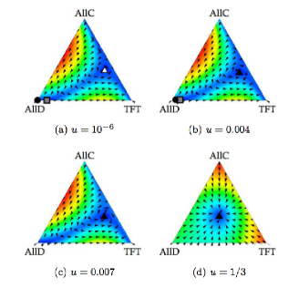
Figure 1: (Color online) Fixed-point structure and flow fields of the standard replicator-mutator equations for the iterated PD at $c=0.8$ and $w=1$. Black symbols are stable fixed points, white symbols are unstable and gray symbols denote saddle points. The AllD fixed point and saddle point can be seen in the bottom left-hand corner of the simplices. The mixed fixed point (triangle) changes stability at $u_{c}^{(1)}\approx 0.0016$. The AllD fixed point (circle) and the saddle point (square) annihilate at $u_{c}^{(2)}\approx 0.005$. Arrows indicate the direction of the deterministic flow in the strategy simplex. The color map shows the Euclidean speed of the trajectories, $||\dot{\bm{x}}||$. These images were produced using a modified version of the Dynamo package Sandholm and Dokumaci (2007).

III.1 General fixed point structure

The qualitative picture one finds is similar for any of the four dynamics; two different threshold values of the mutation rate can be identified, we will refer to these as $u_{c}^{(1)}$ and $u_{c}^{(2)}$. For $0<u<u_{c}^{(1)}$, one typically finds three fixed points: a locally stable attractor near AllD, a saddle point also near AllD, and an unstable fixed point, located close to the AllD/TFT edge of the strategy simplex, see Fig. 1(a). Following Imhof et al. (2005) we will refer to this latter fixed point as the ‘mixed fixed point’. At $u=u_{c}^{(1)}$ the mixed fixed point becomes stable, as shown in panel (b) of Fig. 1. At $u=u_{c}^{(2)}$, the two fixed points near AllD annihilate, leaving the mixed fixed point as the only attractor for $u>u_{c}^{(2)}$, see Fig. 1(c). At $u=1/3$ the mixed fixed point is at or near the center of the simplex, see Fig. 1(d). At this maximal physical meaningful value of $u$ an individual of any type produces an offspring of any of the three different strategies with equal probability. While this qualitative picture is the same for all four dynamics considered here, the numerical values of $u_{c}^{(1)}$ and $u_{c}^{(2)}$ will in general be different for the different dynamics, and they may also depend on the choice of the complexity cost, $c$. The overall picture is consistent with the results of Imhof et al. (2005), where the standard replicator dynamics were studied and where similar qualitative behavior was found. Our analysis thus demonstrates that the findings of Imhof et al. (2005) generalize to a broader class of dynamics. The only difference between our findings compared to those of earlier analyses, lies in the saddle point described above, which was not reported in Imhof et al. (2005), presumably because it is not an attractor of the dynamics. Although for completeness we have given a general account of the fixed point structure, the mixed fixed point will be the focus of our analysis in the following sections, as it is this fixed point which gives rise to coherent oscillations induced by demographic noise.

III.2 Limit of small mutation rates

Further analytical progress is possible in the limit of small mutation rates, $u\ll 1$. For all four cases considered here the deterministic dynamics, derived from Eqs. (13), are of the form

$$\dot{\bm{x}}=\mathbf{h}_{(0)}(\bm{x})+u\mathbf{h}_{(1)}(\bm{x}),$$ (23)

with the mutation rate entering linearly in the resulting differential equations. We will now make the following ansatz for a fixed point $\bm{x}^{*}$:

$$\bm{x}^{*}=\bm{x}_{(0)}^{*}+u\bm{x}_{(1)}^{*},$$ (24)

in the limit of small mutation rates $u$. Here $\bm{x}_{(0)}^{*}$ is a fixed point of Eq. (13) at $u=0$ and $\bm{x}_{(1)}^{*}$ captures the effect of non-zero mutation rates at next-to-leading order. Inserting Eq. (24) into the fixed-point condition

$$\mathbf{h}_{(0)}(\bm{x}^{*})+u\mathbf{h}_{(1)}(\bm{x}^{*})=0,$$ (25)

and collecting terms in linear in $u$, one then finds

$$\bm{x}_{(1)}^{*}=-J^{-1}\bm{h}_{(1)}(\bm{x}_{(0)}^{*}),$$ (26)

where $J$ is the Jacobian of $\mathbf{h}_{(0)}$ evaluated at $\bm{x}^{*}=\bm{x}_{(0)}^{*}$. Since $\bm{x}^{*}_{(0)}$ can be found in closed form from Eqs. (13) with $u=0$, substituting, Eq. (26) into Eq. (24) gives an analytical prediction of the location of the fixed point at small $u$.

In Fig. 2 we compare the outcome of the above linear expansion with results from a direct numerical evaluation of the fixed points of Eq. (13) obtained using a Newton-Raphson procedure. The expansion is seen to be a good approximation for the location of the fixed point for values of $u$ up to $u\approx 0.01$. From the figure we see that the AllD and saddle fixed points annihilate at $u_{c}^{(2)}\approx 0.005$ for this value of $c$. This annihilation is consistent with the disappearance of the AllD fixed point at large $u$ reported by Imhof et al Imhof et al. (2005).

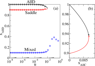
Figure 2: (Color online) Panel (a) shows the $x_{AllD}$ components of the three fixed points of the Moran dynamics at $c=0.8$ with changing mutation rate $u$. Circles are the results from numerically solving the fixed-point equations (25), lines are from Eq. (24). Panel (b) shows the paths of the AllD fixed point and saddle point in phase space as $u$ is varied. The fixed points meet and annihilate at $u\approx 0.005$, for $u$ larger than this value neither fixed point is present.

III.3 Mixed fixed point and phase diagram

For suitable choices of the model parameters $c$ and $u$, the mixed fixed point can be a stable attractor with complex eigenvalues of the corresponding Jacobian. One can thus expect coherent stochastic oscillations to arise in finite populations at those model parameters. We therefore focus our attention on the mixed fixed point, and identify the regions in the $(c,u)$-plane where such complex eigenvalues are found. More generally we will determine the nature of the mixed fixed point as a function of $u$ and $c$. The result of numerically solving for fixed points of the deterministic dynamics corresponding to the Moran process is shown in Fig. 3. We will denote fixed points with purely real eigenvalues as ‘nodes’ and those with complex eigenvalues as ‘spirals’. At low values of $c$ we observe a re-entry phenomenon, where the mixed fixed point goes from a stable spiral to a stable node and back to a stable spiral as $u$ is decreased.

Numerically we also observe a region where the dynamics converges onto a limit cycle. We are at this point unable to provide a proof for the existence of limit cycles or to analytically determine the position of the border between the limit cycle and unstable spiral regions. We therefore determine the presence of limit cycles by numerically integrating the deterministic dynamics using an Euler forward method, starting from the center of the simplex, allowing for a period of equilibration and then applying a suitable threshold criterion to detect closed trajectories. The unstable spiral region is identified as the region where we do not find limit cycles numerically. In situations where there is more than one attractor (e.g. a limit cycle and a stable fixed point near AllD) initial conditions will determine the stationary state of the dynamics. At $u=1/3$ the mixed fixed point is located in the center of the strategy simplex, and becomes a stable node.

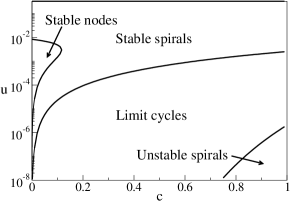
Figure 3: A phase diagram showing the regions in the $(c,u)$ plane for which the mixed fixed point of Eq. (13) for the Moran process is a stable node, stable spiral, unstable spiral or is orbited by a limit cycle. The solid line at $u=1/3$ indicates that at this value the mixed fixed point becomes a stable node situated at $\bm{x}=(1/3,1/3)$. Note that due to the procedure used to check for the presence of limit cycles, the border between the limit cycle and unstable spiral regions is only approximate.

All other update rules studied in this paper have the same qualitative features as the Moran process, and hence their phase diagrams are structurally similar to that shown in Fig. 3, except that the mixed fixed point does not become a stable node at $\bm{x}=(1/3,1/3)$ at $u=1/3$ for rules that use pairwise comparison. Instead, the fixed point forms a stable spiral close to the center of the simplex. Although qualitative features of the phase diagrams are the same for all four update rules, the quantitative positions of the borders in the $(c,u)$ plane may differ for each update rule. For example, Fig. 4 shows the stability map for the Fermi process. Here the re-entry region persists for larger values of $c$ and the region in which the mixed fixed point is unstable is also much larger.

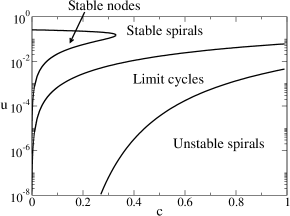
Figure 4: Phase diagram for the Fermi process. We again see the same qualitative structure as for the other update rules, with a difference only in the positions of the boundaries.

IV Stochastic effects and system-size expansion

Until now we have focused on the dynamics of infinite populations. In this section we investigate effects arising in finite populations, especially stochastic oscillations arising via a coherent amplification of intrinsic fluctuations. Such oscillations have been found in a variety of systems as described in the introduction. These quasi-cycles typically arise in regions of the phase diagram where the deterministic dynamics approach a fixed point, and so the range of parameters in which systems of finite populations display oscillations is generally wider than the region in which the deterministic system allows for periodic solutions. Fig. 5 indeed confirms that this is also the case for the evolutionary dynamics of the iterated PD. In the figure we choose model parameters such that none of the four deterministic dynamics approach periodic attractors, but instead have stable fixed points with complex eigenvalues (stable spirals). As seen in the figure the dynamics in finite populations still generate oscillatory behavior, induced by intrinsic fluctuations. This oscillatory behavior is similar to that reported in Imhof et al. (2005). The four panels demonstrate that the quality and frequency of these stochastic oscillations can vary over a wide range depending on the details of the microscopic dynamics, and so we will now go on to characterize their properties in more detail in order to obtain a more comprehensive picture of this phenomenon.

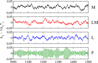
Figure 5: (Color online) The results for the concentration of the AllC strategy from one run of a Gillespie simulation Gillespie (1976, 1977) for each of the four update rules at $N=10000$, $c=0.8$, and $u=0.05$. The time averaged concentration of each run has been subtracted from the data to give the deviation from the deterministic fixed point.

The analytical approach we will use to characterize these fluctuations is based on an expansion of the master equation in the inverse system size van Kampen (2007). This method is now standard in the analysis of interacting-agent systems, and we will therefore not present the full details of the calculation, but instead restrict ourselves to giving a few of the intermediate steps and the final results. The starting point of the system-size expansion is an ansatz of the type

$$\frac{n_{i}}{N}=x_{i}(t)+\frac{1}{\sqrt{N}}\xi_{i}(t),$$ (27)

amounting to a separation of deterministic and stochastic contributions to the number, $n_{i}$, of individuals of type $i$ in the population. The first term on the right, $x_{i}(t)$, is the deterministic trajectory, and $\xi_{i}(t)$ captures fluctuations about this trajectory; the magnitude of these fluctuations is expected to be of order $N^{-1/2}$, as reflected by the above ansatz. One proceeds by inserting this ansatz into the master equation (II.3) and focuses on the probability distribution of $\bm{\xi}$, rather than that of $\mathbf{n}$, so that one sets $P(\bm{n},t)=\Pi(\bm{\xi},t)$. Expanding the resulting master equation for $\Pi(\bm{\xi},t)$ in powers of $N^{-1/2}$ one recovers, at leading order, the generalized replicator-mutator equation, Eq. (13). At next-to-leading order in $N^{-1/2}$ a Fokker-Planck equation of the form

$$\frac{\partial\Pi}{\partial t}=-\sum_{i}\frac{\partial}{\partial\xi_{i}}(C_{i}\Pi)+\frac{1}{2}\sum_{i,j}B_{ij}\frac{\partial^{2}\Pi}{\partial\xi_{i}\partial{\xi_{j}}},$$ (28)

is found van Kampen (2007), where $C_{i}=\sum_{k}J_{ik}\xi_{k}$. Here $J$ is the Jacobian of Eq. (13) and $B$ is a symmetric, $2\times 2$ matrix, whose precise form will depend on the exact nature of the microscopic dynamics, but whose general form is given in Appendix A. The Fokker-Planck equation (28) is equivalent to the linear Langevin equation Gardiner (2009)

$$\dot{\bm{\xi}}=J\bm{\xi}+\bm{\eta},$$ (29)

where $\bm{\eta}$ is Gaussian white noise with correlations

$$\left<\eta_{i}(t)\eta_{j}(t^{\prime})\right>=B_{ij}\delta(t-t^{\prime}).$$ (30)

In contrast to the Langevin equations derived using the Kramers-Moyal expansion Traulsen et al. (2006), Eq. (29) contains additive, rather than multiplicative noise. In the application we are considering here, we are interested in fluctuations about the stationary state and so the matrices $J$ and $B$ are evaluated at the fixed point of the deterministic dynamics.

Given the linearity of Eq. (29), it is straightforward to compute the power spectra of the fluctuations $\bm{\xi}$ about the deterministic fixed point. Following the steps of McKane et al. (2007), one obtains

$$P_{i}(\omega)=\left<|\widetilde{\xi}_{i}(\omega)|^{2}\right>=\sum_{j}\sum_{k}\Phi_{ij}^{-1}B_{jk}(\Phi^{\dagger})^{-1}_{ki},$$ (31)

where $\Phi=i\omega\mathbb{I}-J$ and $\mathbb{I}$ is the $2\times 2$ identity matrix.

In Fig. 6 we give an example of the power spectra of fluctuations about the deterministic fixed point obtained for the Moran update rule at $c=0.8$ ($w=1$), $u=0.01$, and $N=12000$. Theoretical predictions from the van Kampen expansion and numerical simulations are in near perfect agreement. The spectrum shows a pronounced peak at a frequency of approximately $\omega=0.05$, indicating the existence of amplified oscillations with that characteristic frequency. The amplitude of these oscillations is proportional to $N^{-1/2}$, see Eq. (27), the proportionality constant is determined by the area under the power spectrum. Depending on the choice of parameter values one can then expect the amplitude of the quasi-cycle will be of order one up to system sizes of $10^{4}$ or so, i.e. comparable to the species concentrations at the deterministic fixed point. Even for very large populations the oscillations can therefore be significant. If the trajectory of the system is monitored over a time scale much smaller than the oscillation period, then this may lead to intervals in time in which the concentration of AllC is found to be consistently higher than that of TFT or AllD, that is, to intermediate periods where co-operation dominates the population. Such effects may for example be relevant when evolutionary time scales are much longer than time windows over which measurements can be made.

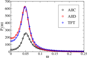
Figure 6: (Color online) The power spectra for oscillations in the concentrations of the three strategies with Moran updating for $c=0.8$ and $u=0.01$. Symbols are the results of a Gillespie simulation with $N=12000$ and approximately $10^{4}$ runs. Solid lines are theoretical predictions obtained from Eq. (31). Simulation results show excellent agreement with the theory.

Having shown that the analytical approach captures the properties of quasi-cycles accurately, we can now compare the magnitude of the stochastic oscillations for the different update processes at the same values of $c$ and $u$. The power spectra of the fluctuations in the AllC concentration are shown in Fig. 7 for the four update rules at one fixed mutation rate and for a specific choice of the complexity cost. Results indicate that the Fermi process produces demographic oscillations of a higher frequency than the other update rules, in line with the time series shown in Fig. 5. Even though the power spectra for the Moran and linear Moran update rules are seemingly indistinguishable in Fig. 7, they are not analytically equivalent.

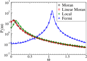
Figure 7: (Color online) A comparison of the power spectra for oscillations in the AllC strategy concentration at $c=0.8$ and $u=0.05$. $N$ ranges from $10^{4}$ to $10^{6}$ and the number of runs for each simulation is of order $10^{4}$.

The magnitude of the peak in the power spectra is a good proxy for the amplitude of the stochastic quasi-cycles, and the height of the peak is in turn largely determined by the inverse of the real part of the relevant eigenvalue of the deterministic dynamics at the fixed point. In the deterministic system, perturbations about the fixed point decay with a time constant proportional to the inverse of this real part, and it is intuitively easy to see that the magnitude of stochastic oscillations diverges as the real part of the largest eigenvalue tends to zero. More specifically, as shown in Boland et al. (2008), the magnitude of the peak in the spectra diverges as the system approaches a Hopf bifurcation, where the stable spiral becomes an unstable one. The resulting delta-function peak in the power spectrum indicates that a limit cycle is born in the unstable phase. This can also be seen from Eq. (31) and the definition of the matrix $\Phi$. At the Hopf bifurcation the relevant eigenvalue of $J$ is purely imaginary, and when $\omega$ becomes equal to the imaginary part of this eigenvalue, the matrix $\Phi$ becomes singular, such that the expression on the right-hand side of Eq. (31), involving the inverse of $\Phi$, diverges.

In order to compare the relative magnitude of stochastic oscillations in the four different dynamics at fixed values of $u$ and $c$, it is therefore useful to determine how far or near to the instability the pair $(u,c)$ places the respective dynamics. In Fig. 8 we plot the instability lines indicating the occurrence of a Hopf bifurcation in the $(u,c)$ plane for the four different types of dynamics. For any fixed $c$ one finds that $u_{c,F}^{(1)}>u_{c,L}^{(1)}>u_{c,LM}^{(1)}>u_{c,M}^{(1)}$ and that accordingly for any $u$ sufficiently large to place all four dynamics in the stable regime, the Fermi process is much closer to the limit-cycle regime than the other types of dynamics, and would therefore be expected to have a larger peak in the power spectra. As discussed above we furthermore find that the Fermi process, with its alternative form of the pairwise comparison process, produces demographic oscillations of a higher frequency than the other update rules, see Fig. 7.

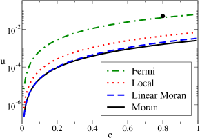
Figure 8: (Color online) The borders between the stable spiral region (above the respective lines) and limit cycle region (below) for the different update processes. The black dot indicates the point $(c,u)=(0.8,0.05)$ used in Fig. 7.

V Iterated prisoner’s dilemma with errors

In this section we study an extended version of the iterated PD game, allowing for a fourth pure strategy, win-stay lose-shift (WSLS). It is appropriate to include this strategy in the discussion when so-called ‘trembling-hand’ errors are considered Imhof et al. (2007). Trembling-hand errors introduce the possibility of a player making a mistake after they have decided what to play, that is, a player co-operating when they meant to defect, or defecting when the intention was to co-operate. We will assume that the two players make errors of this type independently with a small probability $\epsilon>0$ in any given round. TFT’s disadvantage is then that it can become locked into a cycle of alternate co-operation and defection with another TFT player after a mistake occurs. In such games, TFT can be outperformed by WSLS Nowak (2006). WSLS co-operates initially and then keeps using its strategy (co-operation or defection) whenever it receives payoff $T$ or $R$ and switches its strategy (from co-operation to defection or vice versa) if it receives $P$ or $S$. WSLS does not become locked in such cycles when playing against TFT or WSLS. We include the WSLS strategy in our game, extending the dynamics to three degrees of freedom.

In the presence of trembling-hand errors the outcome of a PD game between two fixed players and iterated for a finite number of rounds will generally be stochastic and depend on the timing at which errors occur in the interaction sequence. In order to simplify matters we will therefore follow Imhof et al. (2007) and restrict the discussion to cases in which an interaction between two players consists of an infinite number of iterations of the PD game. It is then appropriate to use the expected payoffs per round, i.e. for two fixed players, say of types $i,j\in\{\mbox{AllC, AllD, TFT, WSLS}\}$, one formally considers an infinite sequence of PD interactions, and uses the mean payoff per round to define the payoff matrix elements $a_{ij}$. The payoff matrix can then be worked out for small error rates, and is given in Imhof et al. (2007) and reproduced in Appendix B for convenience. The complexity cost, $c$, is no longer a relevant parameter now that the number of rounds is infinite.

Previous work on this game has shown that in the limits of zero mutation and weak selection the population can either fix on WSLS or AllD depending on the values used in the payoff matrix Imhof et al. (2007). We continue to use the parameter values given in Sec. II.1 and explore how the dynamics of the game depend on mutation and error rates and identify and classify demographic oscillations. Analyzing the four update rules given in Sec. II.3 we again find a mixed fixed point on which we focus our analysis — since demographic oscillations may occur about this fixed point when it is a stable spiral. We use Eq. (13) with four strategies to track the location and stability properties of the mixed fixed point as $u$ is varied. The path of the mixed fixed point at constant $\epsilon$ and changing $u$ for the Moran process, is shown in Fig. 9. The dashed lines are the result of a similar perturbative expansion to that carried out in Sec. III, where again we see good agreement with numerical results for changes in $u$ up to $u\approx 0.01$.

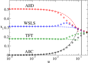
Figure 9: (Color online) The AllC, AllD, TFT and WSLS components of the mixed fixed point for the infinitely iterated PD for changing $u$ at $\epsilon=10^{-4}$. Microscopic dynamics are of the Moran type. Dashed lines are analytical results from a linear expansion in $u$, circles are from a numerical evaluation of the fixed point. The vertical solid black line indicates the location of $u_{c}^{(1)}$, i.e. the value of $u$ where the mixed fixed point changes stability.

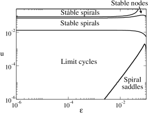
Figure 10: The stability of the mixed fixed point for Moran updating in the infinitely iterated PD game in the $(\epsilon,u)$ plane. Note that the border between the limit cycle and spiral saddle regions is approximate.

Similar to our analysis of the three-strategy game, we can determine the stability of the mixed fixed point as a function of the model parameters $\epsilon$ and $u$. The classification of the nature of the fixed points is more involved for the four-strategy game, however, as we are analyzing a three-dimensional dynamical system. Stable spirals are now fixed points with one pair of complex-conjugate eigenvalues with a negative real part and an additional real-valued negative eigenvalue. If the sign of the real part of the pair of complex-conjugate eigenvalues is opposite to that of the real-valued eigenvalue we will refer to the fixed point as a spiral saddle Sprott (2003). Fixed points with three real-valued negative eigenvalues of the Jacobian are referred to as stable nodes. The resulting phase diagram for the Moran dynamics is shown in Fig. 10. The other three types of microscopic dynamics give qualitatively similar phase diagrams, but the exact quantitative positions of the various phase lines will generally be different.

When the mixed fixed point is a spiral saddle the deterministic dynamics can either converge to a limit cycle or to the attractor at AllD, depending on initial conditions. For locations in the parameter space where the mixed fixed point of the deterministic dynamics is a stable spiral, we again observe demographic oscillations, and they can be characterized analytically in a manner similar to that discussed in the previous section. We depict the resulting power spectra for the Moran process in Fig. 11. As seen in the figure WSLS and AllD in particular undergo strong demographic oscillations, with a comparable magnitude between the two strategies.

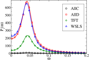
Figure 11: (Color online) The power spectra for the four strategies with Moran updating at $u=0.02$ and $\epsilon=0.01$. Symbols are results from numerical simulations at $N=12000$, solid lines are the predictions of Eq. (31).

As with the iterated PD considered earlier, the amplitude of quasi-cycles resulting from an amplification of intrinsic fluctuations can be expected to be large when a fixed point of the stable spiral type is located close to the border between the stable-spiral and limit-cycle phases. There can then again be periods in time when WSLS is the most prevalent strategy, despite AllD dominating the fixed point. The power spectra for oscillations in the concentration of the TFT strategy resulting from the four different update rules are compared in Fig. 12. We again observe that the Fermi process exhibits oscillations of a higher frequency and with a larger amplitude than the other rules. Although spectra for the local process and the Fermi process overlap in the figure, this is coincidental at this point in parameter space, and will not be the case in general.

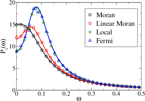
Figure 12: (Color online) The oscillations in the TFT strategy concentration for the four update rules at $u=0.05$ and $\epsilon=10^{-4}$. Symbols are from simulations, lines from the theory. System sizes in the range $N=10^{4}$ to $10^{6}$ are used. For this particular choice of parameters, the spectra for the local and Fermi processes overlap, although this is not the case in general.

VI Conclusion and outlook

In this paper we have used analytical approaches based on van Kampen’s system-size expansion to study the emergence of quasi-cycles in evolutionary games in finite populations. Most existing studies of such effects are of a numerical nature; we have complemented these giving a systematic account of the formalism, and derived the resulting effective Langevin equations which describe the statistics and correlations of fluctuations in large, but finite populations. This approach and our general formulae are applicable to a large class of microscopic update rules, and to games with an arbitrary number of pure strategies. They are, in principle, also valid for arbitrary mutation matrices. The results of this paper hence allow one to predict the regions in parameter space in which coherent quasi-cycles are to be expected, and to compute their spectral properties. In particular coherent cycles, such as reported in game dynamical systems e.g. in Imhof et al. (2005), can be understood as a consequence of the combination of intrinsic noise and the existence of a stable fixed point with complex eigenvalues in the corresponding deterministic system obtained in the limit of infinite populations. In absence of noise the deterministic system approaches such fixed points in an oscillatory manner, with oscillations dying away at a rate proportional to the inverse real part of the relevant eigenvalue. In finite systems, discretization noise leads to persistent stochastic corrections perturbing the system at all times. In the limit of large, but finite system sizes these fluctuations (the noise $\bm{\eta}$ in Eq. (29), together with the pre-factor $N^{-1/2}$) can be seen as a small perturbation to the deterministic dynamics, driving the system away from the fixed point. The attracting fixed point and the oscillatory approach to it on the deterministic level on the one hand and the persistent intrinsic noise on the other then conspire to give coherent and sustained stochastic cycles, with an amplitude largely determined by the inverse real part of the least stable complex eigenvalue.

We have applied the van Kampen formalism to the specific example of the iterated PD game, where stochastic oscillations have been reported in the earlier numerical study Imhof et al. (2005). We have worked out detailed phase diagrams depicting the nature of the limiting deterministic dynamics and we have studied systematically how the mutation rate and complexity cost, the two main model parameters, affect the outcome of the deterministic system. Based on this analysis we are able to predict the parameter regimes in which stochastic oscillations occur. In particular we find that oscillation amplitudes become maximal when the Hopf bifurcation line in the phase diagram is approached from within the stable phase. At the bifurcation line the oscillation amplitude formally diverges, with the power spectrum turning into a delta-function, and as the instability line is crossed a limit cycle is born.

We have also carried out a detailed comparison of four different microscopic update rules; results indicate that their respective phase diagrams are qualitatively similar. The analysis shows that, at fixed values of the model parameters, the Fermi process tends to produce stochastic cycles with larger amplitudes and frequencies than the other update rules. We have extended our study to a version of the iterated PD game in which errors of the trembling-hand type occur with a small, but non-zero rate. The so-called win-stay lose-shift strategy has here been seen to out compete tit-for-tat, and accordingly we have considered a four-strategy space (always defect, always co-operate, tit-for-tat and win-stay lose-shift), and have identified the regions in parameter space where coherent cycles are most likely to occur. Analytical results for the resulting power spectra of these quasi-cycles are confirmed convincingly in numerical simulations.

Mathematical techniques of the type we have used here, most notably the master equation formalism and system-size expansions, were first devised in statistical physics, but they are becoming increasingly more popular in the game theory literature. This extends to equivalent approaches based on Kramers-Moyal expansions. We attribute this popularity to the generality with which these methods are applicable and to the fact that they allow one to obtain an exhaustive account of the properties of first-order stochastic corrections to the limiting deterministic dynamics. Exact analytical results can be derived for large, but finite populations, and hence these techniques make simulations on the microscopic level redundant (at least in principle). We expect this to be the case for games with more complicated strategy structures, or with interaction between more than two players such as for example in public goods games. The analytical approach can also be expected to be applicable to other, potentially more intricate types of human error. For such games it may be difficult or time consuming to carry out reliable simulations and to perform exhaustive parameter searches. Analytical characterizations of stochastic effects such as the ones discussed in this paper may then be particularly welcome.

Appendix A System-size expansion of the master equation

The van Kampen system-size expansion has been extensively discussed elsewhere, together with explicit examples McKane and Newman (2005); Alonso et al. (2007); van Kampen (2007), and so here we will only briefly summarize the general idea and give the final results of the calculation that are relevant for this paper.

The starting point is the substitution of the ansatz (27) into the master equation (II.3) — or its generalization to more than three strategies. This yields an expansion in powers of $N^{-1/2}$, after a re-scaling of time by a factor of $N$. To leading order ($N^{-1/2}$) the deterministic equation (13) is obtained. To next-to-leading order ($N^{-1}$) the Fokker-Planck equation (28) is found. This is defined in terms of two quantities: $C_{i}=\sum_{k}J_{ik}\xi_{k}$, where $J$ is the Jacobian of the dynamics given by Eq. (13), and $B$ a symmetric matrix. Since we are interested in fluctuations about stationary states, both $J_{ij}$ and $B_{ij}$ are time-independent.

The Jacobian can be obtained in a straightforward fashion once the dynamics (13) is known. The elements of the matrix $B$ are found from the $N^{-1}$ terms in the system-size expansion to be

$$B_{ij}=\left\{\begin{array}[]{l l}\sum_{k\neq i}\left[T_{i\to k}(\bm{x})+T_{k\to i}(\bm{x})\right]\,,&\quad\mbox{if $i=j$}\\ \\ -\left[T_{i\to j}(\bm{x})+T_{j\to i}(\bm{x})\right]\,,&\quad\mbox{if $i\neq j$}\\ \end{array}\right..$$ (32)

Therefore the deterministic and stochastic dynamics to the order we are working are entirely determined by $T_{i\to j}(\bm{x})$. This can be found by making the substitutions $(n_{i}/N)\to x_{i}$, $f_{i}\to f_{i}^{\infty}$ and $\phi\to\phi^{\infty}$ in Eq. (10), to obtain

$$T_{i\rightarrow j}(\bm{x})=\sum_{k}x_{k}x_{i}g_{ki}(\bm{f}^{\infty})q_{kj}.$$ (33)

This explicitly shows how to construct $T_{i\rightarrow j}(\bm{x})$, once the process (defined by $g_{ki}(\bm{f})$) and the mutation matrix ($q_{ij}$) have been given.

Appendix B Payoff matrix for a four strategy, infinitely repeated PD with trembling hand errors

When two players meet and play the PD game over multiple rounds their state in round $\ell$ is defined by their actions in that round, e.g. player $1$ co-operates, player $2$ defects. The actions of the pair of players then determines the payoff they each receive. The payoff matrix for the infinitely repeated PD game with trembling hand errors is constructed by considering the stationary distributions of the state of each pair of players, to first order in $\epsilon$, the probability of a ‘trembling hand’ error occurring Imhof et al. (2007). It is given by

$$\bordermatrix{&AllC&AllD&TFT&WSLS\cr AllC&R-\epsilon(2R-S-T)&S+\epsilon(R+P-2S)&R-\epsilon(3R-T-2S)&(R+S)/2+(\epsilon/2)\alpha\cr AllD&T-\epsilon(2T-R-P)&P+\epsilon(S+T-2P)&P+\epsilon(S+2T-3P)&(P+T)/2-(\epsilon/2)\alpha\cr TFT&R+\epsilon(2T+S-3R)&P+\epsilon(T+2S-3P)&\gamma&\gamma\cr WSLS&(R+T)/2+(\epsilon/2)\beta&(P+S)/2-(\epsilon/2)\beta&\gamma&R+\epsilon(T+2P+S-4R)\cr}.$$ (34)

where $\alpha=(T+P-R-S)$, $\beta=(S+P-R-T)$ and $\gamma=(T+R+P+S)/4$.