Robustness of nuclear core activity reconstruction by data assimilation

Abstract

We apply a data assimilation techniques, inspired from meteorological applications, to perform an optimal reconstruction of the neutronic activity field in a nuclear core. Both measurements, and information coming from a numerical model, are used. We first study the robustness of the method when the amount of measured information decreases. We then study the influence of the nature of the instruments and their spatial repartition on the efficiency of the field reconstruction.

Keywords: Data assimilation, Schur complement, neutronic, activities reconstruction, nuclear in-core measurements

1 Introduction

In this paper, we focus on the efficiency of a neutronic field reconstruction procedure with Data Assimilation when varying the number and the repartition of the available instruments. The data assimilation technique used for this reconstruction allows to combine, in an optimal and consistent way, information coming either from measurements or from a numerical model.

Data assimilation methods are not commonly used in nuclear core physics [1], contrary to meteorology or oceanography [2, 3, 4]. The procedure proposed here is the same as the one meteorologists use to obtain high accuracy meteorological reconstructed fields in time and space. This is the case, for example, of the commonly used meteorological re-analysis data set ERA-40 [5] among others [6, 7].

One of the main advantages of data assimilation is that it takes into account every kind of heterogeneous information within the same framework. Moreover, this method has a formalism that allows to adapt itself to instrument configuration change. We exploit this last property here to study the quality of the reconstructed activity field as a function of the number of available measurements. A major point in this study is to estimate the instrumented system robustness in the framework of a data assimilation reconstruction procedure. Moreover, such a study also informs about the effect of instrumentation design within a nuclear core and the resilience to instrument removal.

In this paper, we first detail the data assimilation method and how it addresses field reconstruction. To evaluate the influence of the number of instruments on the activity field reconstruction, the repeated application of the method faces some huge computational issues. Those difficulties are overcomed using a matrix inversion method based on the Schur complement. A detailed presentation of this method is presented in Appendix A. First we present the results on a standard case with synthetic measurements and comments on them. To get a better understanding, we extend the results to other instrumental repartitions and other errors settings. This allows us to give some conclusions on the error and instrument repartition effects in activity field reconstruction using data assimilation.

2 Data assimilation

We briefly introduce the useful data assimilation key points to understand their use as applied in [8, 9, 10]. Data assimilation is a wider domain and these techniques are, for example, the keys of the nowadays meteorological operational forecasts [11]. This is through advanced data assimilation methods that weather forecasting has been drastically improved during the last 30 years. All the available data, such as satellite measurements as well as sophisticated numerical models, are used.

The ultimate goal of data assimilation methods is to estimate the inaccessible true value of the system state, $\mathbf{x}^{t}$ where the $t$ index stands for ”true state” in the so called ”control space”. The basic idea is to combine information from an a priori on the state of the system (usually called $\mathbf{x}^{b}$, with $b$ for ”background”), and measurements (referenced as $\mathbf{y}^{o}$). The background is usually the result of numerical simulations, but can also be derived from any a priori knowledge. The result of data assimilation is called the analysis, denoted by $\mathbf{x}^{a}$, and it is an estimation of the true state $\mathbf{x}^{t}$ we want to approximate.

The control and observation spaces are not necessary the same, and a bridge between them needs to be built. This is the observation operator $H$, that transforms values from the space of the background to the space of observations. For our data assimilation purpose we will use its linearisation $\mathbf{H}$ around the background. The inverse operation going from observation increments to background increments is given by the transpose $\mathbf{H}^{T}$ of $\mathbf{H}$.

Two other ingredients are necessary. The first one is the covariance matrix of observation errors, defined as $\mathbf{R}=E[(\mathbf{y}^{o}-H(\mathbf{x}^{t})).(\mathbf{y}^{o}-H(\mathbf{x}^{t}))^{T}]$ where $E[.]$ is the mathematical expectation. It can be obtained from the known errors on unbiased measurements which means $E[\mathbf{y}^{o}-H(\mathbf{x}^{t})]=0$. The second one is the covariance matrix of background errors, defined as $\mathbf{B}=E[(\mathbf{x}^{b}-\mathbf{x}^{t}).(\mathbf{x}^{b}-\mathbf{x}^{t})^{T}]$. It represents the error on the a priori state, assuming it to be unbiaised following the $E[\mathbf{x}^{b}-\mathbf{x}^{t}]=0$ no biais property. There are many ways to get this a priori state and background error matrices. However, those matrix are commonly the output of a model and an evaluation of accuracy, or the result of expert knowledge.

It can be proved, within this formalism, that the Best Unbiased Linear Estimator (BLUE) $\mathbf{x}^{a}$, under the linear and static assumptions, is given by the following equation:

$$\mathbf{x}^{a}=\mathbf{x}^{b}+\mathbf{K}\big{(}\mathbf{y}^{o}-H\mathbf{x}^{b}\big{)},$$ (1)

where $\mathbf{K}$ is the gain matrix:

$$\mathbf{K}=\mathbf{B}\mathbf{H}^{T}(\mathbf{H}\mathbf{B}\mathbf{H}^{T}+\mathbf{R})^{-1}.$$ (2)

Moreover, we can get the analysis error covariance matrix $\mathbf{A}$, characterising the analysis errors $\mathbf{x}^{a}-\mathbf{x}^{t}$. This matrix can be expressed from $\mathbf{K}$ as:

$$\mathbf{A}=(\mathbf{I}-\mathbf{K}\mathbf{H})\mathbf{B},$$ (3)

where $\mathbf{I}$ is the identity matrix.

It is worth noting that solving Equation 1 is, if the probability distribution is Gaussian, equivalent to minimise the following function $J(\mathbf{x})$, $\mathbf{x}^{a}$ being the optimal solution:

$$J(\mathbf{x})=(\mathbf{x}-\mathbf{x}^{b})^{T}\mathbf{B}^{-1}(\mathbf{x}-\mathbf{x}^{b})\vskip 6.0pt plus 2.0pt minus 2.0pt+\big{(}\mathbf{y}^{o}-\mathbf{H}\mathbf{x}\big{)}^{T}\mathbf{R}^{-1}\big{(}\mathbf{y}^{o}-\mathbf{H}\mathbf{x}\big{)}.$$ (4)

This minimisation is known in data assimilation as 3D-Var methodology [8].

3 Data assimilation implementation

The framework of this study is the standard configuration of a 900 MWe nuclear Pressurized Water Reactor (PWR900). To perform data assimilation, both simulation code and data are needed. For the simulation code, the EDF experimental calculation code for nuclear core COCAGNE in a standard configuration is used. The description of the basic features of this model are done in Section 3.1.

To have a good understanding of the instrumentation effect, we want to study various kind of configurations, even some that do not exist operationally and so cannot be tested experimentally. For that purpose, synthetic data are used that allows to have an homogeneous approach all along the document. Synthetic data is generated from a model simulation, filtered through an instrument model and noised according to a predefined measurement error density function (usually of Gaussian type).

Figure 1: The positions of MFC instruments in the nuclear core are localised in assemblies in black within the horizontal slice of the core. The assemblies without instrument are marked in white and the reflector, out of the reactive core, is in gray.

In the present case, we study the activity field reconstruction. An horizontal slice of a PWR900 core is represented on the Figure 1. There is a total of $157$ assemblies within this core. Among those assemblies, $50$ are instrumented with Mobiles Fissions Chambers (MFC). Those assemblies are divided verticaly in $29$ vertical levels. Thus, the size of the control $\mathbf{x}$ is $4553$ $(157\times 29)$. The size of the observation vector $\mathbf{y}^{o}$ is $1450$ $(50\times 29)$.

3.1 Brief description of the nuclear core model

The aim of a neutronic code like COCAGNE is to evaluate the neutronic activity field and all associated values within the nuclear core. This field depend on the position in the core and on the neutron energy. To do such an evaluation, the population of neutrons are divided in several groups of energy. In the present case only two groups are taken into account giving the neutronic flux $\Phi=(\Phi_{1},\Phi_{2})$ (even if the present code have no limit for the group number). The material properties depend on the position in the core, as the neutronic flux $\Phi$, identified by solving two-group diffusion equations described by:

$$\left\{\begin{array}[]{l}\displaystyle-\mbox{div}(D_{1}\mbox{{grad}}\Phi_{1})+(\Sigma_{a1}+\Sigma_{r})\Phi_{1}=\frac{1}{k}\Big{(}\nu_{1}\Sigma_{f1}\Phi_{1}+\nu_{2}\Sigma_{f2}\Phi_{2}\Big{)}\\ \displaystyle-\mbox{div}(D_{2}\mbox{{grad}}\Phi_{2})+\Sigma_{a2}\Phi_{2}-\Sigma_{r}\Phi_{1}=0,\\ \end{array}\right.$$ (5)

where $k$ is the effective neutron multiplication factor, all the quantities and the derivatives (except $k$) depend on the position in the core, $1$ and $2$ are the group indexes, $\Sigma_{r}$ is the scattering cross section from group $1$ to group $2$, and for each group, $\Phi$ is the neutron flux, $\Sigma_{a}$ is the absorption cross section, $D$ is the diffusion coefficient, $\nu\Sigma_{f}$ is the corrected fission cross section.

The cross sections also depend implicitly on the concentration of boron, which is a substance added in the water used for the primary circuit to control the neutronic fission reaction, throught a feedback supplementary model. This model takes into account the temperature of the materials and of the neutron moderator, given by external thermal and thermo-hydraulic models. A detailed description of the core physic and numerical solving can be found in reference [12].

The overall numerical resolution consists in searching for boron concentration such that the eigenvalue $k$ is equal to $1$, which means that the nuclear power production is stable and self-sustaining. It is named critical boron concentration computation.

The activity in the core is obtained through a combination of the fluxes $\Phi=(\Phi_{1},\Phi_{2})$, given on the chosen mesh of the core. Using homogeneous materials for each assembly (for example $157$ in a PWR900 reactor), and choosing a vertical mesh compatible with the core (usually $29$ vertical levels), this result in a field of activity of size $157\times 29=4553$ that cover all the core.

3.2 The observation operator $H$

The $H$ observation operator is the composition of a selection and of a normalisation procedure. The selection procedure extracts the values corresponding to effective measurement among the values of the model space. The normalisation procedure is a scaling of the value with respect to the geometry and power of the core. The overall operation is non linear. However, with a range of value compatible with assimilation procedure, we can calculate the linear associated operator $\mathbf{H}$. This observation matrix is a $(4553\times 1450)$ matrix.

3.3 The background error covariance matrix $\mathbf{B}$

The $\mathbf{B}$ matrix represents the covariance between the spatial errors for the background. In order to get those, we estimate them as the product of a correlation matrix $\mathbf{C}$ by a normalisation factor.

The correlation $\mathbf{C}$ matrix is built using a positive function that defines the correlations between instruments with respect to a pseudo-distance in model space. Positive functions have the property (via Bochner theorem) to build symmetric defined positive matrix when they are used as matrix generator [13, 14]. In the present case, Second Order Auto-Regressive (SOAR) function is used to prescribe the $\mathbf{C}$ matrix. In such a function, the amount of correlation depends from the euclidean distance between spatial points. The radial and vertical correlation length ($L_{r}$ and $L_{z}$ respectively, associated to the radial $r$ coordinate and the vertical $z$ coordinate) have different values, which means we are dealing with a global pseudo euclidean distance. The used function can be expressed as follow:

$$C(r,z)=\left(1+\frac{r}{L_{r}}\right)\left(1+\frac{|z|}{L_{z}}\right)\exp{\left(-\frac{r}{L_{r}}-\frac{|z|}{L_{z}}\right)}.$$ (6)

The matrix obtained by the above Equation 6 is a correlation matrix. It is then multiplied by a suitable variance coefficient to get covariance matrix. This coefficient is obtained by statistical study of difference between model and measurements in real case. In our case, the size of the $\mathbf{B}$ matrix is related to the size of model space so it is $(4553\times 4553)$.

3.4 The observation error covariance matrix $\mathbf{R}$

The observation error covariance matrix $\mathbf{R}$ is approximated by a diagonal matrix. This means it is assumed that no significant correlation exists between the measurement errors of the MFC. The usual modelling is to take those value as a percentage of the observation. This can be expressed as:

$$\mathbf{R}_{jj}=\left(\alpha(y^{o})_{j}\right)^{2},\quad\forall j$$ (7)

The parameter $\alpha$ is fixed according to the accuracy of the measurement and the representative error associated to the instrument. The size of the $\mathbf{R}$ matrix is related to the size of observation space, so it is $(1450\times 1450)$.

4 General results on instrument removal

To test the robustness, many BLUE calculations need to be done to evaluate the results quality with instruments configuration modifications. We want to have an evaluation of the quality of reconstruction as a function of the number of instruments, with a significant statistical result. To efficiently perform these numerous computations, a specific method using Schur complement was developped. The details of this new method are reported in Appendix A.

Here, we are interested in the evaluation of the quality of the analysis $\mathbf{x}^{a}$ as a function of the amount of provided information. To quantify this effect we make a statistic of $200$ scenarios of instruments removal. We are making those statistics on several hypothesis, starting from a complete instrument configuration and then removing instruments two by two until none remains. The calculation are done on the basis of the algorithm and hypothesis on data assimilation described previously.

To quantify the impact of removed instruments on the analysis, we look at the percentage quantity $v$ defined as follow:

$$v=100\frac{||\mathbf{y}^{o}_{ref}-H\mathbf{x}^{b}||-||\mathbf{y}^{o}_{ref}-H\mathbf{x}^{a}||}{||\mathbf{y}^{o}_{ref}-H\mathbf{x}^{b}||-||\mathbf{y}^{o}_{ref}-H\mathbf{x}^{a}_{ref}||},$$ (8)

where $\mathbf{x}^{a}_{ref}$ corresponds to the analysis when no instrument is removed (this is the best estimation possible with respect to the information available on the system), and where $\mathbf{y}^{o}_{ref}$ and $H$ are the reference observations and observation operator used to build $\mathbf{x}^{a}_{ref}$. $H$ stand for the observation operator when no instrument are removed. This criterium, which is basd on the norm of the innovation vector $\mathbf{y}^{o}_{ref}-H\mathbf{x}^{b}$, focuses on measurements. Since $||\mathbf{y}^{o}_{ref}-H\mathbf{x}^{a}||$ is greater than $||\mathbf{y}^{o}_{ref}-H\mathbf{x}^{a}_{ref}||$ (best estimate) and smaller than $||\mathbf{y}^{o}_{ref}-H\mathbf{x}^{b}||$ (innovation), $v$ is a measure of the quality of the analysis.

Such a definition have several advantages. First of all, the limit of this function are interesting. On the one hand, limit when no instrument is removed is $100\%$. On the other hand, the limit when all instruments are removed is $0\%$. With such a formula we can compare the variation of the information on a unique scale. If we obtain some value above the limit of $100\%$, this mean the parametrisation of data assimilation was not done correctly.

The interest of using this formula is that it can be applied directly as well to experimental data as to synthetic data without any change.

On Figure 2 are presented the results of the quantity $v$ as a function of the number of removed instruments.

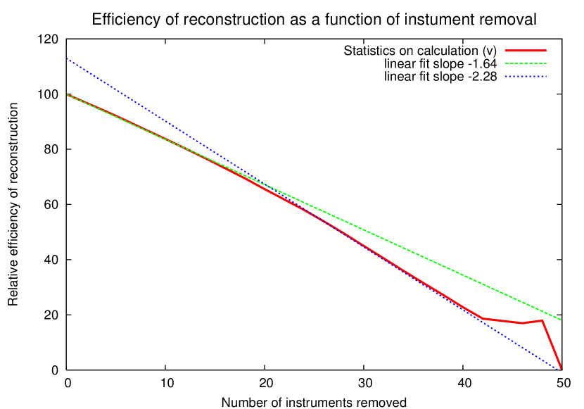
Figure 2: The plain curve represents the value $v$ given by Equation 8 as a function of the number of instruments removed. This results come from a typical PWR900 instrument location. The two other lines are linear regression corresponding to both decreasing regime.

As expected, the relative quality of reconstruction decreases as a function of the number of instruments removed. However within this decrease, three phases can be seen:

1. A first phase of slow decreasing until we removed roughly $20$ instruments. This phase is rather clear and can be fitted by a linear regression with a slope of $-1.64$ (arbitrary unit (a.u.) per instrument). The fit is shown in (green) dash line on Figure 2.

2. After $20$ instrument removed the decreasing speed of the slope increases. The second linear fit has a slope of $-2.28$ (a.u. per instrument). This fit is shown in (blue) dotted line in Figure 2.

3. Beyond $40$ instruments removed, we reach a third phase of stagnation then a brutal decrease to $0$ the limit value imposed by Equation 8.

This characteristic behaviour can be seen in several cases that we studied. We have also noticed it on real measurements [15, 16]. The transition between the two first decreasing phases is specially strong when we do the analysis using real measurements.

First, we explain why the third phase is marked by a stagnation of the mean value of $||\mathbf{y}^{o}-\mathbf{H}\mathbf{x}^{a}||$ over the set of removal scenarios taken into account. To understand that effect, we work on both the cases where two instruments are removed (i.e 48 are remain), and the ones where two instruments are remaining. On those two cases, at most $1225$ scenarios are possibles, corresponding to the $C^{50}_{2}$ combinations. Using the hybrid Schur method, we can calculate all those cases with a rather cheap computing time to obtain a good statistics. We plotted the distribution of the value of $||\mathbf{y}^{o}-\mathbf{H}\mathbf{x}^{a}||$ over all the scenarios in Figure 3.

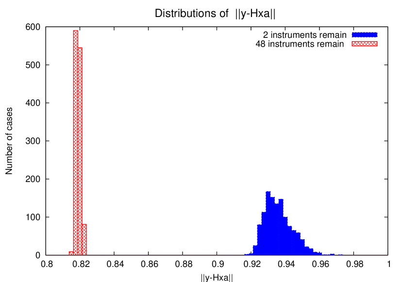
Figure 3: Distribution of the norms of $||\mathbf{y}^{o}-\mathbf{H}\mathbf{x}^{a}||$ for all the cases where only two instruments are suppressed or two instruments remain in the instrument network on a PWR900 reactor.

On the Figure 3 we notice a big difference between the two distributions plotted, that correspond to the cases where two instruments are removed (i.e. $48$ remain) or two remain.

The shifting of the mean value between those two extreme cases is logical as available information is dramatically changing. However, the shape of the distribution is also vastly changing. We move from a very sharp distribution, when $48$ instruments remain, to a rather broad one when two instruments remain.

The first interesting point of this shape change is that all the instruments do not have the same influence on the activity field reconstruction. To understand better this effect let’s assume that all the instruments are equivalent. In this case, as the number of scenarios present in the two distributions of Figure 3 are the same, only a shifting of the mean value should have be seen. However we have not only a translation of the distribution but also a broadening. Thus, there is a non equivalence of instruments within the data assimilation procedure, in terms of marginal information assigned to each instrument, depending on its location in the core

The second point of interest is that the broadening of the distribution is asymmetric. The distribution extends towards the higher values of norm. This effect explains the stagnation of the $v$ quantity when few instruments remain. The source of stagnation is the discrepancy between the most probable value of the distribution and the mean value of the distribution which is higher. The most probable value leads to a decrease without stagnation. However, looking at the mean value (that has more physical meaning), we see that this one stagnates due to the asymmetric broadening that compensates the overall decrease in mean value.

Now the origin of the two slopes in decreasing of the information represented by the Figure 2 will be investigated. The repartition of the instruments in a standard PWR900 is very complex as shown in Figure 1. This complexity of the repartition does not make the situation easy to understand. Thus, we want to study the case on a simpler repartition of the instrumentation to see if the effect of two phases decreasing persists.

5 Repartition effects in instrument removal

The position of the instruments are presented in Figure 4. The core geometry and assemblies configuration is the same as a PWR900 one, however the instrument are located regularly on a Cartesian map.

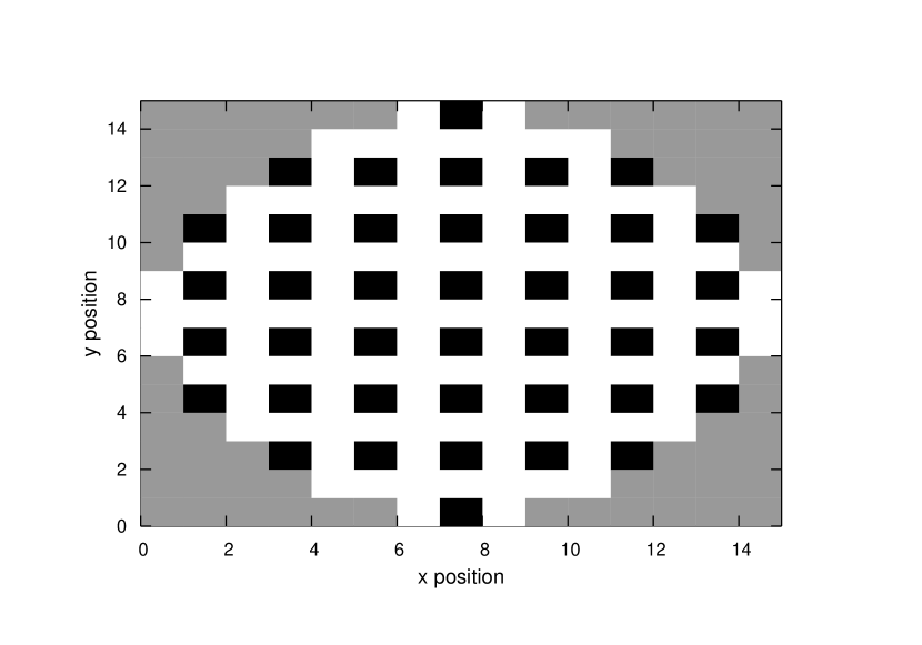
Figure 4: The MFC instruments within the nuclear core are localised in assemblies in black within the horizontal slice of the core. The assemblies without instrument are marked in white and the reflector is in gray.

Within this configuration, only $40$ MFC are used, which is a bit less than $50$ of the standard PWR configuration presented on Figure 1. With this repartition, we do the same analysis as on the previous one. The evolution on $v$ as a function of the number of removed instruments is plotted in Figure 5.

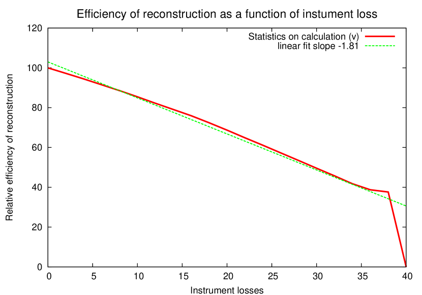
Figure 5: The plain curve represents the value $v$ given by Equation 8 as a function of the number of instruments removed. This results come from a regular instruments location in a PWR900. The dashed line represents the linear fit of the steady part of the curve.

In the Figure 5, the quality of the activity reconstruction decreases quasi-linearly as a function of the number of removed instruments. This goes on until we reach the stagnation phase. It appears, comparing Figure 5 to 2 that the variation of the decrease slope is related to the geometrical repartition of the instruments. Such uniform linear decreasing can be observed also in several other rather geometrically regular repartition, as one with repartition on diagonal line. Some of the repartitions have densities of instruments close to the one of the standard PWR900, which do not change the overall behaviour.

Looking at the slope factor of the linear fit, we notice that the one with regular MFC repartition (Figure 5) is in the range of the slopes obtained with standard MFC repartition (Figure 2).

Thus the removal or fault resilience of the instrument set seems to depend on the transition point between the two decreasing steps. In the lower range of instrumental density, it is better to have a regular repartition, and in the higher one, it is better to have a complex ad-hoc repartition. In real PWR900 nuclear core, because the set of intruments is fixed at a high density level, these results indicate that it is more robust to have an ad-hoc repartition of the instruments as for now.

6 Conclusion

We proposed and studied here an original method to test how the neutronic activity field reconstruction by data assimilation is tolerant to information removal. The core of the reconstruction method is based on data assimilation, that is widely use in earth sciences, and allows a very good reconstruction of the activity all over the nuclear core. An hybrid method for fast matrix inversion partially based on Schur complement allows the execution on numerous analysis from which statistical results are derived. For all these analyses, synthetic data are used to try non-experimental intruments repartitions, but similar results were established using real data. This application on real data prove both the reliability and the quality of the calculation code and the data assimilation methodology.

Using those advanced calculation methods, it was shown that the slopes of the reconstruction quality is mainly governed by repartition for the instruments. Depending on the chosen repartition, the decrease consists in two or three distinct phases. The ultimate stagnation phase in this decreasing is governed by both statistical effect and heterogeneity of instruments influence.

The behaviour with two phases within the decreasing quality of the reconstruction as a function of the number of instruments removed is understood in term of repartition effect, but not quantified. However it can be seen as a phase transition between two states of instrumental configuration. The quantification of this transition is worth studying.

Appendix A Appendix: Schur complement method to optimise calculation

Within the BLUE assimilation method, the limiting factor in calculation time is the matrix inversions. In Equation 2, the costly part is the inversion of the term:

$$\mathbf{M}=\mathbf{H}\mathbf{B}\mathbf{H}^{T}+\mathbf{R}.$$ (9)

The inversion cost on huge matrix as $\mathbf{M}$ (around $4000\times 4000$ in the present case) was such that the time calculation of the above evaluation was extremely time consuming. Then we had to optimise the computing cost.

We noticed that the calculations are more time consuming when only few instruments are removed. In this case the $\mathbf{M}$ matrix is still huge.

Thus, the idea is to use the information obtained in the inversion of the full size matrix to shorten calculation, to calculate smaller size matrix in a reasonable time. In this case, we want to calculate the new matrix as a perturbation of the original one. Such a method exists and exploits the Schur complement of the matrix.

We assume we want to suppress some instruments to a given configuration. With respect to the Equation 2, we need to calculate a new matrix $\mathbf{K}_{n}$. The $n$ index is standing for referring the new matrix we want to calculate. For that according to Equation 9 we have to determine a new matrix $\mathbf{M}_{n}$.

This determination of $\mathbf{M}_{n}$ is obtained from the knowledge of the invert of the matrix $\mathbf{M}_{g}$ calculated over all the instruments. The indices $g$ is used to denote the reference matrix we start from $\mathbf{M}_{g}$ according to Equation 9.

All the components of the new matrix $\mathbf{K}_{n}$ can be obtained by suppressing the lines and columns corresponding to removed instruments in $\mathbf{M}_{g}$, inverting it and then multiplying this matrix by the corresponding $\mathbf{H}_{n}$ and $\mathbf{B}_{n}$. We notice that, in our case, we get $\mathbf{B}_{n}=\mathbf{B}_{g}$ as we do not affect the model space.

To make the demonstration easier, but without losing any generality, we can assume that the suppressed instruments correspond to the lower square of $\mathbf{M}_{g}$. If it is not the case, it is always possible to reorganise matrix in such a way.

Now we put the $\mathbf{M}_{g}$ under a convenient form, separating remaining measures from removed ones. Assuming the starting matrix $\mathbf{M}_{g}$ is $m\times m$ and that we plan so suppress $s$ measurements, we can write $\mathbf{M}_{g}$ in the following way:

$$\mathbf{M}_{g}=\left(\begin{array}[]{cc}\mathbf{P}_{g}&\mathbf{Q}_{g}\\ \mathbf{R}_{g}&\mathbf{S}_{g}\end{array}\right),$$ (10)

where:

• $\mathbf{P}_{g}$ contains the remaining measurements, and is a $p\times p$ matrix,

• $\mathbf{S}_{g}$ contains the suppressed measurement, and is a $s\times s$ matrix,

• $\mathbf{Q}_{g}$ et $\mathbf{R}_{g}$ represent the dependence between remaining measured and suppressed ones. In the particular case we are dealing with, we have $\mathbf{Q}_{g}^{T}=\mathbf{R}_{g}$. However, no further use of this property is done.

  With such a decomposition, we got the equality $m=p+s$.

The $\mathbf{P}_{g}$ matrix corresponds to the remaining instruments, thus we have the equality:

$$\mathbf{P}_{g}=\mathbf{M}_{n},$$ (11)

The decomposition given in Equation 10 is the one required to build the Schur complement of this matrix [17]. Under the condition that $\mathbf{P}_{g}$ can be inverted, the Schur complement is the following quantity:

$$\mathbf{S}_{g}-\mathbf{R}_{g}\mathbf{P}_{g}^{-1}\mathbf{Q}_{g},$$ (12)

and is noted $(\mathbf{M}_{g}/\mathbf{P}_{g})$. This notation reads as Schur complement of $\mathbf{M}_{g}$ by $\mathbf{P}_{g}$.

Thus we look for a cheap way to calculate $\mathbf{P}_{g}^{-1}$ knowing $\mathbf{M}_{g}^{-1}$. For that, we use the Banachiewiz formula [17] that gives invert of $\mathbf{M}_{g}$ as a function of $\mathbf{P}_{g}$, $\mathbf{Q}_{g}$, $\mathbf{R}_{g}$, $\mathbf{S}_{g}$ and $(\mathbf{M}_{g}/\mathbf{P}_{g})$ matrices:

$$\mathbf{M}_{g}^{-1} = \left(\begin{array}[]{cc}\mathbf{P}_{g}&\mathbf{Q}_{g}\\ \mathbf{R}_{g}&\mathbf{S}_{g}\end{array}\right)^{-1}$$ (15)

$$= \left(\begin{array}[]{cc}\mathbf{P}_{g}^{-1}+\mathbf{P}_{g}^{-1}\mathbf{Q}_{g}(\mathbf{M}_{g}/\mathbf{P}_{g})^{-1}\mathbf{R}_{g}\mathbf{P}_{g}^{-1}&-\mathbf{P}_{g}^{-1}\mathbf{Q}_{g}(\mathbf{M}_{g}/\mathbf{P}_{g})^{-1}\\ -(\mathbf{M}_{g}/\mathbf{P}_{g})^{-1}\mathbf{R}_{g}\mathbf{P}_{g}^{-1}&(\mathbf{M}_{g}/\mathbf{P}_{g})^{-1}\end{array}\right)$$ (18)

We define the 4 sub-matrices $\mathbf{\tilde{P}}_{g}$, $\mathbf{\tilde{Q}}_{g}$, $\mathbf{\tilde{R}}_{g}$ and $\mathbf{\tilde{S}}_{g}$ by:

$$\mathbf{\tilde{P}}_{g} = \mathbf{P}_{g}^{-1}+\mathbf{P}_{g}^{-1}\mathbf{Q}_{g}(\mathbf{M}_{g}/\mathbf{P}_{g})^{-1}\mathbf{R}_{g}\mathbf{P}_{g}^{-1},$$ (19)

$$\mathbf{\tilde{Q}}_{g} = -\mathbf{P}_{g}^{-1}\mathbf{Q}_{g}(\mathbf{M}_{g}/\mathbf{P}_{g})^{-1},$$ (20)

$$\mathbf{\tilde{R}}_{g} = -(\mathbf{M}_{g}/\mathbf{P}_{g})^{-1}\mathbf{R}_{g}\mathbf{P}_{g}^{-1},$$ (21)

$$\mathbf{\tilde{S}}_{g} = (\mathbf{M}_{g}/\mathbf{P}_{g})^{-1}.$$ (22)

Rearranging those terms we get:

$$\mathbf{P}_{g}^{-1}=\mathbf{\tilde{P}}_{g}-\mathbf{\tilde{Q}}_{g}\mathbf{\tilde{S}}_{g}^{-1}\mathbf{\tilde{R}}_{g}.$$ (23)

As by hypothesis we know the inverse $\mathbf{M}_{g}^{-1}$ of the global matrix, we are able to extract $\mathbf{\tilde{P}}_{g}$, $\mathbf{\tilde{Q}}_{g}$, $\mathbf{\tilde{R}}_{g}$ and $\mathbf{\tilde{S}}_{g}$ from the whole inverted matrix. Thus, the main cost to obtain the inverse of $\mathbf{P}_{g}$ of size $p\times p$ becomes the one of inverting $\mathbf{\tilde{S}}_{g}$ which size is $q\times q$. In first approximation, if the number of measurements to suppress is smaller than the number of remaining one, this methods gives a notable gain. As soon as the matrix $\mathbf{P}_{g}^{-1}=\mathbf{M}_{n}^{-1}$, final calculation of $\mathbf{K}_{n}$ is straightforward.

To highlight the advantages of this method with respect to the standard inversion of sub-matrix, some tests are shown on a $4000\times 4000$ full semi-definite positive regular matrix. The curves showing the effective computing time in percentage of the computing time of the full matrix are presented in Figure 6.

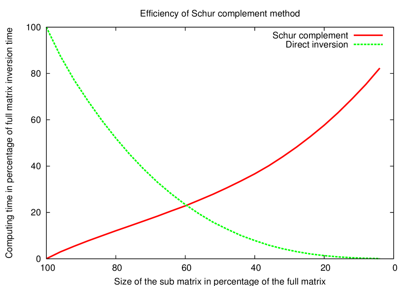
Figure 6: Calculation time as a function of the size of the sub-matrix. Calculation time is given as a percentage of the calculation time of the full size matrix. The size of the sub-matrix is given a a percentage of the size of the full matrix. The curves in full line (red) and in dashed line (green) represent the inversion by Schur complement and direct inversion respectively.

Figure 6 shows that, when sub-matrix has roughly the size of the initial matrix, the inversion by Schur complement is far more efficient than the direct inversion. Above around $60\%$ of the size of the initial matrix, the direct inversion becomes more efficient. The crossing point is at $60\%$ instead of $50\%$, as expected in first approximation. This difference comes from the few additional multiplications that need to be done in the Schur complement calculation, as we can see in Equation 12. Globally, we see that the most efficient method is to use an hybrid calculation that choose the best way to make the calculation as a function of the number of measurements removed. To quantify the improvement of such an hybrid choice, we integrate the curves of direct inversion and compare it to the integral of hybrid option (minimum of both cases) within the instrument loss range. The ratio in percentage of both integrals shows that benefit of this hybrid method represents an overall gain of $64\%$ with respect to standard method.

References

- [1] Sébastien Massart, Samuel Buis, Patrick Erhard, and Guillaume Gacon. Use of 3DVAR and Kalman filter approaches for neutronic state and parameter estimation in nuclear reactors. Nuclear Science and Engineering, 155(3):409–424, 2007.
- [2] David F. Parrish and John C. Derber. The national meteorological center’s spectral statistical interpolation analysis system. Monthly Weather Review, 120:1747–1763, 1992.
- [3] Ricardo Todling and Stephen E. Cohn. Suboptimal schemes for atmospheric data assimilation based on the kalman filter. Monthly Weather Review, 122:2530–2557, 1994.
- [4] Kayo Ide, Philippe Courtier, Michael Ghil, and Andrew C. Lorenc. Unified notation for data assimilation: operational, sequential and variational. Journal of the Meteorological Society of Japan, 75(1B):181–189, 1997.
- [5] S. M. Uppala and et al. The ERA-40 re-analysis. Quaterly Journal of the Royal Meteorological Society, 131(612, Part B):2961–3012, 2005.
- [6] E. Kalnay and et al. The NCEP/NCAR 40-year reanalysis project. Bulletin of American Meteorological Society, 77:437–471, 1996.
- [7] G. J. Huffman and et al. The global precipitation climatology project (GPCP) combined precipitation dataset. Bulltin of American Meteorological Society, 78:5–20, 1997.
- [8] Olivier Talagrand. Assimilation of observations, an introduction. Journal of the Meteorological Society of Japan, 75(1B):191–209, 1997.
- [9] Eugenia Kalnay. Atmospheric Modeling, Data Assimilation and Predictability. 2003.
- [10] Fran ois Bouttier and Philippe Courtier. Data assimilation concepts and methods. Meteorological training course lecture series, ECMWF, March 1999.
- [11] F. Rabier, H. Järvinen, E. Kilnder, J.F. Mahfouf, and A. Simmons. The ECMWF operational implementation of four-dimensional variational assimilation. part I: Experimental results with simplified physics. Quarterly Journal of the Royal Meteorological Society, 126:1143–1170, 2000.
- [12] James J. Duderstadt and Louis J. Hamilton. Nuclear reactor analysis. John Wiley & Sons, 1976.
- [13] Georges Matheron. La théorie des variables régionalisées et ses applications. Cahiers du Centre de Morphologie Mathématique de l’ENSMP, Fontainebleau, Fascicule 5, 1970.
- [14] Denis Marcotte. Géologie et géostatistique minières (cours), 2008.
- [15] Jean-Philippe Argaud, Bertrand Bouriquet, Patrick Erhard, Guillame Gacon, and Sébastien Massart. Exploitation optimale des mesures neutroniques pour l’évaluation de l’état des coeurs de centrales nucléaires, SFP conference, 9-13 july 2007, 2007.
- [16] Jean-Philippe Argaud, Bertrand Bouriquet, Patrick Erhard, Sébastien Massart, and Sophie Ricci. Data assimilation in nuclear power plant core. In ECMI Conference, London, 30 June-4 July 2008. IMA, 2008.
- [17] Fuzhen Zhang. The Schur complement and its applications. Springer, 2005.