On the determination of the nonlinearity from localized measurements in a reaction-diffusion equation

Abstract

This paper is devoted to the analysis of some uniqueness properties of a classical reaction-diffusion equation of Fisher-KPP type, coming from population dynamics in heterogeneous environments. We work in a one-dimensional interval $(a,b)$ and we assume a nonlinear term of the form $u\,(\mu(x)-\gamma u)$ where $\mu$ belongs to a fixed subset of $C^{0}([a,b])$. We prove that the knowledge of $u$ at $t=0$ and of $u$, $u_{x}$ at a single point $x_{0}$ and for small times $t\in(0,\varepsilon)$ is sufficient to completely determine the couple $(u(t,x),\mu(x))$ provided $\gamma$ is known. Additionally, if $u_{xx}(t,x_{0})$ is also measured for $t\in(0,\varepsilon)$, the triplet $(u(t,x),\mu(x),\gamma)$ is also completely determined. Those analytical results are completed with numerical simulations which show that, in practice, measurements of $u$ and $u_{x}$ at a single point $x_{0}$ (and for $t\in(0,\varepsilon)$) are sufficient to obtain a good approximation of the coefficient $\mu(x).$ These numerical simulations also show that the measurement of the derivative $u_{x}$ is essential in order to accurately determine $\mu(x)$.

Keywords: reaction-diffusion $\cdot$ heterogeneous media $\cdot$ uniqueness $\cdot$ inverse problem

1 Introduction and ecological background

Reaction-diffusion models (hereafter RD models), although they sometimes bear on simplistic assumptions such as infinite velocity assumption and completely random motion of animals [1], are not in disagreement with certain dispersal properties of populations observed in natural as well as experimental ecological systems, at least qualitatively [2, 3, 4, 5]. In fact, since the work of Skellam [6], RD theory has been the main analytical framework to study spatial spread of biological organisms, partly because it benefits from a well-developed mathematical theory.

The idea of modeling population dynamics with such models has emerged at the beginning of the 20${}^{\hbox{th}}$ century, with random walk theories of organisms, introduced by Pearson and Blakeman [7]. Then, Fisher [8] and Kolmogorov, Petrovsky, Piskunov [9] independently used a reaction-diffusion equation as a model for population genetics. The corresponding equation is

$$\frac{\partial u}{\partial t}-D\frac{\partial^{2}u}{\partial x^{2}}=u\,(\mu-\gamma u),\ t>0,\ x\in(a,b)\subset\mathbb{R},$$ (1.1)

where $u=u(t,x)$ is the population density at time $t$ and space position $x$, $D$ is the diffusion coefficient, and $\mu$ and $\gamma$ respectively correspond to the constant intrinsic growth rate and intraspecific competition coefficients. In the 80’s, this model has been extended to heterogeneous environments by Shigesada et al. [10]. The corresponding model is of the type:

$$\frac{\partial u}{\partial t}-\frac{\partial}{\partial x}\left(D(x)\frac{\partial u}{\partial x}\right)=u\,(\mu(x)-\gamma(x)u),\ t>0,\ x\in(a,b).$$ (1.2)

The coefficients $\mu(x)$ and $\gamma(x)$ now depend on the space variable $x$ and can therefore include some effects of environmental heterogeneity. More recently, this model revealed that the heterogeneous character of the environment played an essential role on species persistence and spreading, in the sense that for different spatial configurations of the environment, a population can survive or become extinct and spread at different speeds, depending on the habitat spatial structure ([2], [11], [12],[13], [14] ,[15], [16]). Thus, determining the coefficients in model (1.2) is an important question, even for areas other than ecology (see [17] and references therein).

In this paper, we focus on the case of constant coefficients $D$ and $\gamma$:

$$\frac{\partial u}{\partial t}-D\frac{\partial^{2}u}{\partial x^{2}}=u\,(\mu(x)-\gamma u),\ t>0,\ x\in(a,b),$$ (1.3)

and we address the question of the uniqueness of couples $(u,\mu(x))$ and triples $(u,\mu(x),\gamma)$ satisfying (1.2), given a localized measurement of $u$.

Uniqueness results of this type have been obtained for reaction-diffusion models, through the Lipschtiz stability of the coefficient with respect to the solution $u$. Lipschtiz stability is generally obtained by using the method of Carleman estimates [18]. Several publications starting from the paper by Isakov [19] and including the recent overview of the method of Carleman estimates applied to inverse coefficients problems [20] provide results for the case of multiple measurements. The particular problem of the uniqueness of the couple $(u,\mu(x))$ satisfying (1.3) given such multiple measurements has been investigated, together with Lipschtiz stability, in a previous work [21]. Placing ourselves in a bounded domain $\Omega$ of $\mathbb{R}^{N}$ with Dirichlet boundary conditions, we had to use the following measurements: (i) the density $u(0,x)$ in $\Omega$ at $t=0$; (ii) the density $u(t,x)$ for $(t,x)\in(t_{0},t_{1})\times\omega$, for some times $0<t_{0}<t_{1}$ and a subset $\omega\subset\subset\Omega$; (iii) the density $u(\theta,x)$ for all $x\in\Omega$, at some time $\theta\in(t_{0},t_{1})$.

Although the result of [21] allows to determine $\mu(x)$ using partial measurements of $u(t,x),$ assumption (iii) implies that $u$ has to be known in the whole set $\Omega$. This last measurement (iii) is a key assumption in several other papers on uniqueness and stability of solutions to parabolic equations with respect to parameters (see Imanuvilov and Yamamoto [22], Yamamoto and Zou [23], Belassoued and Yamamoto [24] for scalar equations and Cristofol, Gaitan and Ramoul [25] or Benabdallah, Cristofol, Gaitan and Yamamoto [26] for systems).

Here, contrarily to previous results obtained for this type of reaction-diffusion models, there are some regions in $(a,b)$ where $u$ is never measured: we only require to know (i’) the density $u(0,x)$ in $(a,b)$ at $t=0$ and (ii’) the density $u(t,x_{0})$ and its spatial derivative $\displaystyle{\frac{\partial u}{\partial x}}(t,x_{0})$ for $t\in(0,\varepsilon)$ and some point $x_{0}$ in $(a,b)$ (see Remark 2.5 for a particular example of hypothesis (ii’)). Thus a measurement of type (iii) is no more necessary. Furthermore, we show simultaneous uniqueness of two coefficients $\mu(x)$ and $\gamma$ provided that measurements of the second derivative $\displaystyle{\frac{\partial^{2}u}{\partial x^{2}}}(t,x_{0})$ are available.

Our paper is organized as follows: in the next section, we give precise statements of our hypotheses and results; Section 3 is then dedicated to the proof of the results. Section 4 is devoted to the description of numerical examples illustrating how the coefficient $\mu(x)$ can be approached using measures of the type (i’) and (ii’). Those results are further discussed in Section 5.

2 Hypotheses and main results

Let $(a,b)$ be an interval in $\mathbb{R}$. We consider the problem:

$$\left\{\begin{array}[]{l}\frac{\partial u}{\partial t}-D\frac{\partial^{2}u}{\partial x^{2}}=u\,(\mu(x)-\gamma u),\ t\geq 0,\ x\in(a,b),\\ \alpha_{1}u(t,a)-\beta_{1}\frac{\partial u}{\partial x}(t,a)=0,t>0,\\ \alpha_{2}u(t,b)+\beta_{2}\frac{\partial u}{\partial x}(t,b)=0,\ t>0,\\ u(0,x)=u_{i}(x),\ x\in(a,b).\end{array}\right.\hskip 28.45274pt(\mathcal{P}_{\mu,\gamma})$$

Our hypotheses on the coefficients are the following. Firstly, we assume that:

$$\mu\in M:=\{\psi\in C^{0,\eta}([a,b])\hbox{ such that }\psi\hbox{ is piecewise analytic on }(a,b)\},$$ (2.4)

for some $\eta\in(0,1]$. The space $C^{0,\eta}$ corresponds to Hölder continuous functions with exponent $\eta$ (see e.g. [27]). A function $\psi\in C^{0,\eta}([a,b])$ is called piecewise analytic if it exists $n>0$ and an increasing sequence $(i_{k})_{1\leq k\leq n}$ such that $i_{1}=a$, $i_{n}=b$, and

$$\hbox{for all }x\in(a,b),\ \psi(x)=\sum_{j=1}^{n-1}\chi_{[i_{j},i_{j+1})}(x)\varphi_{j}(x),$$

for some analytic functions $\varphi_{j}$, defined on the intervals $[i_{j},i_{j+1}]$, and where $\chi_{[i_{j},i_{j+1})}$ are the characteristic functions of the intervals $[i_{j},i_{j+1})$ for $j=1,\ldots,n-1$.

We also assume that $\gamma$ is a positive constant and that the boundary coefficients satisfy:

$$\alpha_{1},\alpha_{2},\beta_{1},\beta_{2}\geq 0\hbox{ with }\alpha_{1}+\beta_{1}>0\hbox{ and }\alpha_{2}+\beta_{2}>0.$$ (2.5)

We furthermore make the following hypotheses on the initial condition:

$$u_{i}\geq 0,\ u_{i}\not\equiv 0\hbox{ and }u_{i}\in C^{2,\eta}([a,b]),$$ (2.6)

for some $\eta$ in $(0,1)$, that is $u_{i}$ is a $C^{2}$ function such that $u_{i}^{\prime\prime}$ is Hölder continuous. In addition to that, we assume the following compatibility conditions:

$$\alpha_{1}u_{i}(a)-\beta_{1}u_{i}^{\prime}(a)=0,\ \alpha_{2}u_{i}(b)+\beta_{2}u_{i}^{\prime}(b)=0,\ \delta_{\beta_{1}}u_{i}^{\prime\prime}(a)=0,\ \delta_{\beta_{2}}u_{i}^{\prime\prime}(b)=0,$$ (2.7)

where $\delta_{y}$ is verifies: $\delta_{0}=1$ and $\delta_{y}=0$ if $y\neq 0$. We also need to assume that:

$$\hbox{measure}(\{x\in(a,b),\ u_{i}(x)=0\})=0.$$ (2.8)

Under the assumptions (2.4)-(2.7), for each $\mu\in M$ and $\gamma>0$, the problem $(\mathcal{P}_{\mu,\gamma})$ has a unique solution $u\in C^{2,\eta}_{1,\eta/2}([0,+\infty)\times[a,b])$ (i.e. the derivatives up to order two in $x$ and order one in $t$ are Hölder continuous, see [27, 28] for a definition of Hölder continuity). Existence, uniqueness and regularity of the solution $u$ are classical. See e.g. [28, Ch. 1].

Let us state our main results:

Theorem 2.1.

Let $\mu,\tilde{\mu}\in M,$ and $\gamma>0$, and assume that the solutions $u$ and $\tilde{u}$ to $(\mathcal{P}_{\mu,\gamma})$ and $(\mathcal{P}_{\tilde{\mu},\gamma})$ satisfy, at some $x_{0}\in(a,b),$ and for some $\varepsilon>0$ and all $t$ in $(0,\varepsilon)$:

$$u(t,x_{0}) = \tilde{u}(t,x_{0}),$$ (2.9)

$$\frac{\partial u}{\partial x}(t,x_{0}) = \frac{\partial\tilde{u}}{\partial x}(t,x_{0}).$$ (2.10)

Assume furthermore that

$$u_{i}(x_{0})\neq 0\hbox{ or }\frac{\partial^{2}u}{\partial x^{2}}(t,x_{0})=\frac{\partial^{2}\tilde{u}}{\partial x^{2}}(t,x_{0})\hbox{ for }t\in(0,\varepsilon).$$ (2.11)

Then, we have $\mu\equiv\tilde{\mu}$ on $[a,b]$ and consequently $u\equiv\tilde{u}$ in $[0,+\infty)\times[a,b]$. If $\beta_{1}>0$ (resp. $\beta_{2}>0$), this statement remains true when $x_{0}=a$ (resp. $x_{0}=b$).

Remark 2.2.

This result remains valid if $\gamma=\gamma(x)$ is a given, positive function in $C^{0,\eta}([a,b]).$

However, the conclusion of Theorem 2.1 is not true in general without the assumption (2.10):

Proposition 2.3.

Let $\mu\in M$ and $\gamma>0$. Assume that $\alpha_{1}=\alpha_{2}$ and $\beta_{1}=\beta_{2}$ and that $u_{i}$ is symmetric with respect to $x=(a+b)/2.$ Let $\tilde{\mu}:=\mu(b-(x-a))$ for $x\in[a,b].$ Then, the solutions $u$ and $\tilde{u}$ to $(\mathcal{P}_{\mu,\gamma})$ and $(\mathcal{P}_{\tilde{\mu},\gamma})$ satisfy $u(t,\frac{a+b}{2})=\tilde{u}(t,\frac{a+b}{2})$ for all $t\geq 0.$

Under an additional assumption on the initial condition $u_{i}$, we are able to obtain a uniqueness result for triples $(u,\mu,\gamma)$:

Theorem 2.4.

Let $\mu,\tilde{\mu}\in M,$ and $\gamma,\tilde{\gamma}>0$. Assume that, at some $x_{0}\in(a,b)$, $u_{i}(x_{0})=0$. Assume furthermore that the solutions $u$ and $\tilde{u}$ to $(\mathcal{P}_{\mu,\gamma})$ and $(\mathcal{P}_{\tilde{\mu},\tilde{\gamma}})$ satisfy, for some $\varepsilon>0$ and for all $t$ in $(0,\varepsilon)$:

$$u(t,x_{0}) = \tilde{u}(t,x_{0}),$$ (2.12)

$$\frac{\partial u}{\partial x}(t,x_{0}) = \frac{\partial\tilde{u}}{\partial x}(t,x_{0}),$$ (2.13)

$$\frac{\partial^{2}u}{\partial x^{2}}(t,x_{0}) = \frac{\partial^{2}\tilde{u}}{\partial x^{2}}(t,x_{0}).$$ (2.14)

Then, we have $\mu\equiv\tilde{\mu}$ on $[a,b]$ and $\gamma=\tilde{\gamma}$. Consequently $u\equiv\tilde{u}$ in $[0,+\infty)\times[a,b]$. If $\beta_{1}>0$ (resp. $\beta_{2}>0$), this statement remains true for $x_{0}=a$ (resp. $x_{0}=b$).

Remarks 2.5.

• A particular example where hypotheses (2.9-2.11) of Theorem 2.1 (resp. hypotheses (2.12-2.14) of Theorem 2.4) are fulfilled is whenever, for some subset $\omega$ of $(a,b)$, $u(t,x)=\tilde{u}(t,x)$ for $t\in(0,\varepsilon)$ and all $x\in\omega$ (resp. $x_{0}\in\omega$ and $u(t,x)=\tilde{u}(t,x)$ in $(0,\varepsilon)\times\omega$). Note that, under this hypothesis, the previous results [21] did not imply uniqueness; indeed, an additional assumption of type (iii) was required (cf. the introduction section).

• The uniqueness result of Theorem 2.4 cannot be adapted to the stationary equation associated to $(\mathcal{P}_{\mu,\gamma})$: $-p^{\prime\prime}=p\,(\mu(x)-\gamma p)$ (see e.g. [11] for the existence and uniqueness of the stationary state $p>0$). Indeed, for any $\tau\in(0,1),$ setting $\tilde{\mu}=\mu-\tau\gamma p$ and $\tilde{\gamma}=(1-\tau)\gamma$, we obtain $-p^{\prime\prime}=p\,(\tilde{\mu}(x)-\tilde{\gamma}p)$, whereas $\tilde{\mu}\not\equiv\mu$ and $\tilde{\gamma}\not\equiv\gamma$. Thus, a measurement of $p$, even on the whole interval $[a,b]$, does not provide a unique couple $(\mu,\gamma)$.

• The subset $M$ of $C^{0,\eta}([a,b])$ made of piecewise analytic functions is much larger than the set of analytic functions on $[a,b]$. It indeed contains some functions whose regularity is not higher than $C^{0,\eta}$, and some functions which are constant on some subsets of $[a,b]$. Our results hold true if $M$ is replaced by any subset $M^{\prime}$ of $C^{0,\eta}([a,b])$ such that for any couple of elements in $M^{\prime}$, the subset of $[a,b]$ where these two elements intersect has a finite number of connected components.

3 Proofs

Let $\mu,\tilde{\mu}\in M,$ and $\gamma,\tilde{\gamma}>0$. Let $u$ be the solution to $(\mathcal{P}_{\mu,\gamma})$ and $\tilde{u}$ the solution to $(\mathcal{P}_{\tilde{\mu},\tilde{\gamma}})$. We set

$$U:=u-\tilde{u}\hbox{ and }m:=\mu-\tilde{\mu}.$$

The function $U$ satisfies:

$$\frac{\partial U}{\partial t}-D\frac{\partial^{2}U}{\partial x^{2}}=\tilde{\mu}U-\tilde{\gamma}U(u+\tilde{u})+u(m-u(\gamma-\tilde{\gamma})),$$ (3.15)

for $t\geq 0$ and $x\in(a,b),$ and

$$\left\{\begin{array}[]{l}\alpha_{1}U(t,a)-\beta_{1}\frac{\partial U}{\partial x}(t,a)=0,\ \alpha_{2}U(t,b)+\beta_{2}\frac{\partial U}{\partial x}(t,b)=0,\ t>0,\\ U(0,x)=0,\ x\in(a,b).\end{array}\right.$$ (3.16)

Proof of Theorem 2.1: In that case $\gamma=\tilde{\gamma}$. Equation (3.15) then reduces to

$$\frac{\partial U}{\partial t}-D\frac{\partial^{2}U}{\partial x^{2}}=\tilde{\mu}U-\gamma U(u+\tilde{u})+u\,m.$$ (3.17)

Step 1: We prove that $m(x_{0})=0.$

It follows from hypothesis (2.9) that, for all $t\in[0,\varepsilon)$, $U(t,x_{0})=0$ and thereby,

$$\frac{\partial U}{\partial t}(t,x_{0})=0\hbox{ for all }t\in[0,\varepsilon).$$

If $u_{i}(x_{0})\neq 0$, then, since $U(0,\cdot)\equiv 0$ we deduce from (3.17) applied at $t=0$ and $x=x_{0}$ that $u_{i}(x_{0})m(x_{0})=0,$ and therefore $m(x_{0})=0$.

If $u_{i}(x_{0})=0$, from (2.11), we have $\frac{\partial^{2}U}{\partial x^{2}}(t,x_{0})=0$ for all $t\in[0,\varepsilon)$. Applying equation (3.17) at $t=\varepsilon/2$ and $x=x_{0},$ we get

$$u\left(\frac{\varepsilon}{2},x_{0}\right)m(x_{0})=0.$$

If $x_{0}\in(a,b)$, the strong parabolic maximum principle (Corollary 5.2) applied to $u$ implies that $u(\varepsilon/2,x_{0})>0$. As a consequence we again get $m(x_{0})=0$. Lastly, if $x_{0}=a$ and $\beta_{1}>0$ the Hopf’s Lemma applied to $u$ again implies that $u(\varepsilon/2,x_{0})>0$. Indeed, assume on the contrary that $u(\varepsilon/2,x_{0})=u(\varepsilon/2,a)=0$. The boundary condition $\alpha_{1}u(t,a)-\beta_{1}\frac{\partial u}{\partial x}(t,a)=0$ implies:

$$\beta_{1}\frac{\partial u}{\partial x}\left(\frac{\varepsilon}{2},a\right)=0,$$

which is impossible from Hopf’s Lemma (Corollary 5.2 and Theorem 5.1 (b) and (c)). Thus $u(\varepsilon/2,x_{0})>0$ and, again, $m(x_{0})=0$. A similar argument holds for $x_{0}=b$, whenever $\beta_{2}>0.$

Under the assumptions of Theorem 2.1, we therefore always obtain $m(x_{0})=0.$

Step 2: We prove that $m\equiv 0$.

Let us now set

$$b_{1}:=\sup\{x\in[x_{0},b]\hbox{ s.t. }m\hbox{ has a constant sign on }[x_{0},x]\}.$$

By “constant sign” we mean that either $m\geq 0$ on $[x_{0},x]$ or $m\leq 0$ on $[x_{0},x]$. Then, four possibilities may arise:

• (i) $m=0$ on $[x_{0},b_{1}]$ and $b_{1}<b$,

• (ii) $m\geq 0$ on $[x_{0},b_{1}]$ and it exists $x_{1}\in(x_{0},b_{1})$ such that $m(x_{1})>0$,

• (iii) $m\leq 0$ on $[x_{0},b_{1}]$ and it exists $x_{1}\in(x_{0},b_{1})$ such that $m(x_{1})<0$,

• (iv) $b_{1}=b$, and $m=0$ on $[x_{0},b]$.

Assume (i). Then, by definition of $b_{1}$, there exists a decreasing sequence $y_{k}\to b_{1},$ $y_{k}>b_{1}$, such that $|m(y_{k})|>0$ for all $k\geq 0$. Assume that it exists $k_{0}$ such that $|m(x)|>0$ for all $x\in(b_{1},y_{k_{0}})$. By continuity, $m$ does not change sign in $(b_{1},y_{k_{0}})$, and therefore in $[x_{0},y_{k_{0}}]$. This contradicts the definition of $b_{1}$. Thus,

$$\hbox{ for all }k,\hbox{ it exists }z_{k}\in(b_{1},y_{k})\hbox{ such that }m(z_{k})=0.$$ (3.18)

Since $\mu$ and $\tilde{\mu}$ belong to $M$, the function $m$ also belongs to $M$ and is therefore piecewise analytic on $(a,b)$. Thus, the set $\{x\in(a,b)\hbox{ s.t. }m(x)=0\}$ has a finite number of connected components. This contradicts (3.18) and rules out possibility (i).

Now assume (ii). By continuity of $m$, and from hypothesis (2.8) on $u_{i}$, we can assume that $u_{i}(x_{1})>0$. Since $m(x_{1})>0$ and $U(0,\cdot)\equiv 0$, it follows from (3.17) that

$$\frac{\partial U}{\partial t}(0,x_{1})=u_{i}(x_{1})m(x_{1})>0.$$

Thus, for $\varepsilon_{1}>0$ small enough, $U(t,x_{1})>0$ for $t\in(0,\varepsilon_{1}]$. As a consequence, $U$ satisfies:

$$\left\{\begin{array}[]{l}\frac{\partial U}{\partial t}-D\frac{\partial^{2}U}{\partial x^{2}}-(\tilde{\mu}-\gamma u-\gamma\tilde{u})U\geq 0,\ t\in(0,\varepsilon_{1}],\ x\in(x_{0},x_{1}),\\ U(t,x_{0})=0\hbox{ and }U(t,x_{1})>0,\ t\in(0,\varepsilon_{1}],\\ U(0,x)=0,\ x\in(x_{0},x_{1}).\end{array}\right.$$ (3.19)

Moreover,

Lemma 3.1.

We have $U(t,x)>0$ in $(0,\varepsilon_{1})\times(x_{0},x_{1})$.

Proof of Lemma 3.1: Set $W=Ue^{-\lambda t},$ for some $\lambda>0$ large enough such that $c(t,x):=\tilde{\mu}-\gamma u-\gamma\tilde{u}-\lambda\leq 0$ in $(x_{0},x_{1}).$ The function $W$ satisfies

$$\frac{\partial W}{\partial t}-D\frac{\partial^{2}W}{\partial x^{2}}-c(t,x)W\geq 0,\ t\in(0,\varepsilon_{1}],\ x\in(x_{0},x_{1}).$$

Assume that it exists a point $(t^{*},x^{*})$ in $(0,\varepsilon_{1})\times(x_{0},x_{1})$ such that $U(t^{*},x^{*})<0$. Then, since $W(t,x_{0})=0$ and $W(t,x_{1})>0$ for $t\in(0,\varepsilon_{1})$, and since $W(0,x)=U(0,x)=0,$ $W$ admits a minimum $m^{*}<0$ in $(0,\varepsilon_{1}]\times(x_{0},x_{1})$. Theorem 5.1 (a) applied to $W$ implies that $W\equiv m^{*}<0$ on $[0,\varepsilon_{1}]\times[x_{0},x_{1}]$, which is impossible. Thus $W\geq 0$ in $[0,\varepsilon_{1}]\times[x_{0},x_{1}].$ Theorem 5.1 (a) and (c) then implies that $W>0$ and consequently $U(t,x)>0$ in $(0,\varepsilon_{1})\times(x_{0},x_{1})$. $\Box$

Since $U(t,x_{0})=0$, the Hopf’s lemma (Theorem 5.1 (b) and (c)) also implies that $\displaystyle{\frac{\partial U}{\partial x}(t,x_{0})>0}$ for all $t\in(0,\varepsilon_{1}).$ This contradicts hypothesis (2.10). Possibility (ii) can therefore be ruled out.

Applying the same arguments to $-U$, possibility (iii) can also be rejected. Finally, only (iv) remains.

Setting

$$a_{1}:=\inf\{x\in[a,x_{0}]\hbox{ s.t. }m\hbox{ has a constant sign on }[x,x_{0}]\},$$

the same argument as above shows that $a_{1}=a$ and $m=0$ on $[a,x_{0}]$. Thus, finally, $m\equiv 0$ on $[a,b]$ and this concludes the proof of Theorem 2.1. $\Box$

Proof of Theorem 2.4: From the assumptions (2.12) and (2.14) of Theorem 2.4, equation (3.15) at $x=x_{0}$ reduces to

$$u(t,x_{0})\,(m(x_{0})-u(t,x_{0})(\gamma-\tilde{\gamma}))=0\hbox{ for }t\in[0,\varepsilon).$$

If $x_{0}\in(a,b),$ the strong parabolic maximum principle (Corollary 5.2) implies that $u(t,x_{0})>0$ for all $t>0$. This remains true if $x_{0}=a$ (if $\beta_{1}>0$) or $x_{0}=b$ (if $\beta_{2}>0$); cf. the proof of Theorem 2.1. We therefore get:

$$m(x_{0})=u(t,x_{0})(\gamma-\tilde{\gamma})\hbox{ for }t\in(0,\varepsilon).$$ (3.20)

From the continuity of $t\mapsto u(t,x_{0})$ up to $t=0$, we have $m(x_{0})=u_{i}(x_{0})(\gamma-\tilde{\gamma})$. Thus, $u_{i}(x_{0})=0$ implies that $m(x_{0})=0$ which in turns implies from (3.20), and since $u(t,x_{0})>0$ for $t>0$, that $\tilde{\gamma}=\gamma$. The end of the proof is therefore similar to that of Theorem 2.1. $\Box$

Remark 3.2.

Extension of the arguments used in the previous proof to higher dimensions is not straightforward. Indeed, placing ourselves in a bounded domain $\Omega$ of $\mathbb{R}^{N},$ with $N\geq 2$, we may consider the largest region $\Omega_{1}$ in $\Omega$, containing $x_{0}$ and such that $m$ has a constant sign in $\Omega_{1}$. Consider in the above proof the possibility (ii)_N (instead of (ii)): $m\geq 0$ on $\overline{\Omega_{1}}$ and it exists $x_{1}\in\Omega$ such that $m(x_{1})>0$. Then it exists a subset $\omega_{1}$ of $\Omega_{1}$, such that $x_{0}\in\partial\omega_{1}$ and $u(t,x)>0$ on a portion of $\partial\omega_{1}$. However, we cannot assert that $U(t,x)\geq 0$ on $\partial\omega_{1}$, and (ii)_N can therefore not be ruled out as we did for (ii).

Proof of Proposition 2.3: Under the assumptions of Proposition 2.3, we observe that $\tilde{u}(t,b-(x-a))$ is a solution of $(\mathcal{P}_{\mu,\gamma}).$ In particular, by uniqueness, we have

$$u(t,x)=\tilde{u}(t,b-(x-a)),\hbox{ for all }t\geq 0\hbox{ and }x\in[a,b].$$

It follows that $u(t,\frac{a+b}{2})=\tilde{u}(t,\frac{a+b}{2})$ for all $t\geq 0.$ $\Box$

4 Numerical computations

The purpose of this section is to verify numerically that the measurements (2.9-2.10) of Theorem 2.1 allow to obtain a good approximation of the coefficient $\mu(x)$, when $\gamma$ is known.

Assuming that $\mu$ belongs to a finite-dimensional subspace $E\subset M$ and measuring the distance between the measurements of the solutions of $(\mathcal{P}_{\mu,\gamma})$ and $(\mathcal{P}_{\tilde{\mu},\gamma})$ through the function

$$G_{\mu}(\tilde{\mu})=\|u(\cdot,x_{0})-\tilde{u}(\cdot,x_{0})\|_{L^{2}(0,\varepsilon)}+\|\frac{\partial u}{\partial x}(\cdot,x_{0})-\frac{\partial\tilde{u}}{\partial x}(\cdot,x_{0})\|_{L^{2}(0,\varepsilon)},$$

we look for the coefficient $\mu(x)$ as a minimizer of the function $G_{\mu}$. Indeed, $G_{\mu}(\mu)=0$ and, from Theorem 2.1, this is the unique global minimum of $G_{\mu}$ in $M$.

Solving $(\mathcal{P}_{\mu,\gamma})$ by a numerical method (see Appendix B) gives an approximate solution $u^{h}$. In our numerical tests, we therefore replace $G_{\mu}$ by the discretized functional

$$\widehat{G}_{\mu}(\tilde{\mu}):=\|u^{h}(\cdot,x_{0})-\tilde{u}^{h}(\cdot,x_{0})\|_{L^{2}(0,\varepsilon)}+\|\frac{\partial u^{h}}{\partial x}(\cdot,x_{0})-\frac{\partial\tilde{u}^{h}}{\partial x}(\cdot,x_{0})\|_{L^{2}(0,\varepsilon)}.$$

Remark 4.1.

Since $(\mathcal{P}_{\mu,\gamma})$ and $(\mathcal{P}_{\tilde{\mu},\gamma})$ are solved with the same (deterministic) numerical method, we have $\widehat{G}_{\mu}(\mu)=0$. Thus $\mu$ is a global minimizer of $\widehat{G}_{\mu}$. However, this minimizer might not be unique.

4.1 State space $E$

We fix $(a,b)=(0,1)$ and we assume that the function $\mu$ belongs to a subspace $E\subset M$ defined by:

$$E:=\left\{\tilde{\mu}\in C^{0,\eta}([0,1])\,|\,\exists\ (h_{i})_{0\leq i\leq n}\in\mathbb{R}^{n+1},\ \tilde{\mu}(x)=\sum_{i=0}^{n}h_{i}\cdot j\left((n-2)\left(x-c_{i}\right)\right)\hbox{ on }[0,1]\right\},$$

with $c_{i}=\frac{i-1}{n-2}$ and $j(x)=\left\{\begin{array}[]{l}\exp\left(\frac{4x^{2}}{x^{2}-4}\right),\hbox{ if }x\in(-2,2),\\ 0\hbox{ otherwise.}\end{array}\right.$

4.2 Minimization of $\widehat{G}_{\mu}$ in $E$

For the numerical computations, we fixed $D=0.1$, $\gamma=1$, $\alpha_{1}=\alpha_{2}=0$ and $\beta_{1}=\beta_{2}=1$ (Neumann boundary conditions). Besides, we assumed that $u_{i}\equiv 0.2$, $\varepsilon=0.3$ and $x_{0}=2/3.$ The integer $n$ was set to $10$ in the definition of $E$.

Numerical computations were carried out for $100$ functions $\mu_{k}$ in $E:$

$$\mu_{k}=\sum_{i=0}^{n}h_{i}^{k}\cdot j\left[(n-2)\left(x-c_{i}\right)\right],\ k=1\ldots 100,$$

whose components $h_{i}^{k}$ were randomly drawn from a uniform distribution in $(-5,5).$

Minimizations of the functions $\widehat{G}_{\mu_{k}}$ were performed using MATLAB’s^® fminunc solver . This led to $100$ functions $\mu^{*}_{k}$ in $E$, each one corresponding to a computed approximation for a minimizer of the function $\widehat{G}_{\mu_{k}}$. In our numerical tests, we obtained values of $\widehat{G}_{\mu_{k}}(\mu^{*}_{k})$ in $(5\cdot 10^{-7},10^{-5})$, with an average of $5\cdot 10^{-6}$ and a standard deviation of $2\cdot 10^{-6}.$

The values $\|\mu_{k}-\mu^{*}_{k}\|_{L^{2}([0,1])}/\|\mu_{k}\|_{L^{2}([0,1])}$, for $k=1\ldots 100$, are comprised between $5\cdot 10^{-3}$ and $0.16$, with an average value of $0.04$ and a standard deviation of $0.03$.

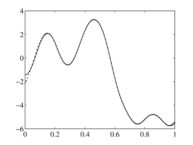
(a) $\mu$ (plain line) and $\mu^{*}$ (dotted line)

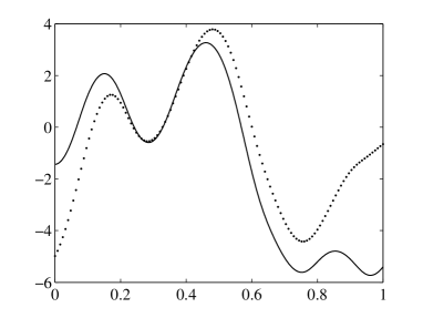
(b) $\mu$ (plain line) and $\underline{\mu}^{*}$ (dotted line)

Figure 1: (a) An example of function $\mu$ in $E$, together with a function $\mu^{*}$ which was obtained by minimizing $\widehat{G}_{\mu}.$ In this case $\|\mu-\mu^{*}\|_{L^{2}([0,1])}/\|\mu\|_{L^{2}([0,1])}=0.03$ and $\widehat{G}_{\mu}(\mu^{*})=2\cdot 10^{-6}$. (b) The same function $\mu$ together with the function $\underline{\mu}^{*}$ obtained by minimizing $\widehat{H}_{\mu}$. Here, $\|\mu-\underline{\mu}^{*}\|_{L^{2}([0,1])}/\|\mu\|_{L^{2}([0,1])}=0.47$ and $\widehat{H}_{\mu}(\underline{\mu}^{*})=2\cdot 10^{-6}.$

Fig. 1 (a) depicts an example of function $\mu$ in $E$, together with a function $\mu^{*}$ which was obtained by minimizing $\widehat{G}_{\mu}.$

4.3 Test of another criterion $H_{\mu}$

In this section, we illustrate that measurement (2.9) alone cannot be used for reconstructing $\mu$. Replacing $G_{\mu}$ by:

$$H_{\mu}(\tilde{\mu})=\|u(\cdot,x_{0})-\tilde{u}(\cdot,x_{0})\|_{L^{2}(0,\varepsilon)},$$

and setting $\widehat{H}_{\mu}(\tilde{\mu}):=\|u^{h}(\cdot,x_{0})-\tilde{u}^{h}(\cdot,x_{0})\|_{L^{2}(0,\varepsilon)},$ we performed the same analysis as above, with the same samples $\mu_{k}\in E$ and the same parameters.

The corresponding values of $\widehat{H}_{\mu}(\underline{\mu}^{*}_{k})$ are comparable to those obtained in Section 4.2. Namely, these values are included in $(2\cdot 10^{-8},10^{-5}),$ with average $2\cdot 10^{-6},$ and standard deviation $3\cdot 10^{-6}.$ However, the corresponding values of the distance $\|\mu_{k}-\underline{\mu}^{*}_{k}\|_{L^{2}([0,1])}/\|\mu_{k}\|_{L^{2}([0,1])}$ are far larger than those obtained in Section 4.2: these values are comprised between $0.08$ and $1.64$, with an average of $0.56$ and a standard deviation of $0.34$.

Using the same sample $\mu\in E$ as in Fig. 1 (a), we present in Fig. 1 (b) the approximation $\underline{\mu}^{*}$ obtained by minimizing $\widehat{H}_{\mu}$. In this case, the distance $\|\mu-\underline{\mu}^{*}\|_{L^{2}([0,1])}/\|\mu\|_{L^{2}([0,1])}$ is $18$ times larger than $\|\mu-\mu^{*}\|_{L^{2}([0,1])}/\|\mu\|_{L^{2}([0,1])}.$

5 Discussion

Studying the reaction-diffusion problem $(\mathcal{P}_{\mu,\gamma})$ with a nonlinear term of the type $u\,(\mu(x)-\gamma u),$ we have proved in Section 2 that knowing $u$ and its first spatial derivative at a single point $x_{0}$ and for small times $t\in(0,\varepsilon)$ is sufficient to completely determine the couple $(u(t,x),\mu(x))$. Additionally, if the second spatial derivative is also measured at $x_{0}$ for $t\in(0,\varepsilon)$, the triplet $(u(t,x),\mu(x),\gamma)$ is also completely determined.

These uniqueness results are mainly the consequences of Hopf’s Lemma and of an hypothesis on the set $M$ of coefficients which $\mu(x)$ belongs to. This hypothesis implies that two coefficients in $M$ can be equal only over a set having a finite number of connected components.

The theoretical results of Section 2 suggest that the coefficients $\mu(x)$ and $\gamma$ can be numerically determined using only measurements of the solution $u$ of $(\mathcal{P}_{\mu,\gamma})$ and of its spatial derivatives at one point $x_{0},$ and for $t\in(0,\varepsilon)$. Indeed, the numerical computations of Section 4 show that, when $\gamma$ is known, the coefficient $\mu(x)$ can be estimated by minimizing a function $G_{\mu}$. The function $\tilde{u}$ being the solution of $(\mathcal{P}_{\tilde{\mu},\gamma}),$ we defined $G_{\mu}(\tilde{\mu})$ as the distance between $(u,\partial u/\partial x)(\cdot,x_{0})$ and $(\tilde{u},\partial\tilde{u}/\partial x)(\cdot,x_{0}),$ in the $L^{2}(0,\varepsilon)$ sense.

The numerical computations presented in Section 4.2 were carried out on $100$ samples of functions $\mu_{k}$ chosen in a finite-dimensional subspace of $M$. In each case, a good approximation $\mu^{*}_{k}$ of $\mu_{k}$ was obtained. The average relative $L^{2}$-error between $\mu^{k}$ and $\mu_{k}^{*}$ is $30$ times smaller than the average relative $L^{2}$-error between $\mu^{k}$ and the constant function $\mu_{k}(x_{0})$. Thus, a measurement of $u$ and of its first spatial derivative at a point $x_{0}$ (and for $t\in(0,\varepsilon)$) indirectly gives more information on the global shape of $\mu$ than a direct measure of $\mu$ at $x_{0}.$ These good results, in spite of the computational error, indicate $L^{2}$-stability of the coefficient $\mu$ with respect to single-point measurements of the solution $u$ of $(\mathcal{P}_{\mu,\gamma})$ and of its spatial derivative.

Proposition 2.3 shows that the uniqueness result of Theorem 2.1 is not true without the assumption (2.10) on the spatial derivatives. This suggests that measurement (2.9) alone cannot be used for reconstructing $\mu.$ In Section 4.3, working with the same samples $\mu_{k}$ as those discussed above, we obtained approximations $\underline{\mu}^{*}_{k}$ of $\mu_{k}$ by minimizing a new function $H_{\mu}$, which measures the distance between $u(\cdot,x_{0})$ and $\tilde{u}(\cdot,x_{0}).$ The average relative $L^{2}$-error between $\mu_{k}$ and $\underline{\mu_{k}}^{*}$ was $14$ times larger than the average relative $L^{2}$-error separating $\mu_{k}$ and $\mu^{*}_{k}.$ This confirms the usefulness of the spatial derivative measurements for the reconstruction of $\mu.$

Appendix A: maximum principle

The following version of the parabolic maximum principle can be found in [27, Ch. 2] and [29, Ch. 3].

Theorem 5.1.

Let $u\in C^{2}_{1}((0,T]\times(x_{1},x_{2}))\cap C([0,T]\times[x_{1},x_{2}]),$ for some $T>0$ and $x_{1},x_{2}\in\mathbb{R}.$ Let $c(t,x)\leq 0\in C^{0,\eta}_{0,\eta/2}([0,T]\times[x_{1},x_{2}])$, for some $\eta\in(0,1]$.

Suppose that $\displaystyle{\frac{\partial u}{\partial t}-D\frac{\partial^{2}u}{\partial x^{2}}-c(x)u\geq 0}$ for $t\in(0,T]$ and $x\in(x_{1},x_{2})$.

(a) If $u$ attains a minimum $m^{*}\leq 0$ at a point $(t^{*},x^{*})\in(0,T]\times(x_{1},x_{2}),$ then $u(t,x)\equiv m^{*}$ on $[0,t^{*}]\times[x_{1},x_{2}]$.

(b) (Hopf’s Lemma) If $u$ attains a minimum $m^{*}\leq 0$ at a point $(t^{*},x_{1})$ (resp. $(t^{*},x_{2})$), with $t^{*}>0$, then either $\frac{\partial u}{\partial x}(t^{*},x_{1})>0$ (resp. $\frac{\partial u}{\partial x}(t^{*},x_{2})<0$) or $u(t,x)\equiv m^{*}$ on $[0,t^{*}]\times[x_{1},x_{2}]$.

(c) If $u\geq 0,$ the results (a) and (b) remain true without the assumption $c(t,x)\leq 0.$

An immediate corollary of this theorem is:

Corollary 5.2.

The solution $u(t,x)$ of $(\mathcal{P}_{\mu,\gamma})$ is strictly positive in $(0,+\infty)\times(a,b)$.

Proof of Corollary 5.2: Assume that it exists $(t^{*},x^{*})\in(0,+\infty)\times(a,b)$ such that $u(t^{*},x^{*})<0$.

Set $w(t,x)=u\,e^{-\lambda t},$ for $\lambda>0$ large enough such that

$$c(t,x):=\mu(x)-\gamma u-\lambda\leq 0\hbox{ in }[0,t^{*}]\times[a,b].$$

The function $w$ satisfies:

$$\frac{\partial w}{\partial t}-D\frac{\partial^{2}w}{\partial x^{2}}-c(t,x)w=0.$$

Since $w(0,x)=u_{i}(x)\geq 0$ in $(a,b)$ and $w(t^{*},x^{*})<0,$ the function $w$ admits a minimum $m^{*}<0$ in $(0,t^{*}]\times[a,b].$ From Theorem 5.1 (a), and since $u_{i}\not\equiv 0,$ this minimum is attained at a boundary point: it exits $t^{\prime}\in(0,t^{*}]$ such that $w(t^{\prime},a)=m^{*}<0$ or $w(t^{\prime},b)=m^{*}<0$. Without loss of generality, we can assume in the sequel that $w(t^{\prime},a)=m^{*}<0.$ From Theorem 5.1 (b), we obtain $\frac{\partial w}{\partial x}(t^{\prime},a)>0.$ Using the boundary conditions in problem $(\mathcal{P}_{\mu,\gamma})$, we finally get:

$$\alpha_{1}\,m^{*}=\beta_{1}\,\frac{\partial w}{\partial x}(t^{\prime},a)>0.$$

Using assumption (2.5), we get a contradiction. Thus $u(t,x)\geq 0$ in $(0,+\infty)\times(a,b).$ The conclusion then follows from Theorem 5.1 (c). $\Box$

Appendix B: numerical solutions of $(\mathcal{P}_{\mu,\gamma})$ and $(\mathcal{P}_{\tilde{\mu},\gamma})$

The equations $(\mathcal{P}_{\mu,\gamma})$ and $(\mathcal{P}_{\tilde{\mu},\gamma})$ were solved using Comsol Multiphysics^® time-dependent solver, using second order finite element method (FEM) with 960 elements. This solver uses a method of lines approach incorporating variable order variable stepsize backward differentiation formulas. Nonlinearities are treated using a Newton’s method. The interested reader can get more information in Comsol Multiphysics^® user’s guide.

References

References

- [1] E E Holmes. Are diffusion models too simple? A comparison with telegraph models of invasion. American Naturalist, 142:779–795, 1993.
- [2] N Shigesada and K Kawasaki. Biological invasions: theory and practice. Oxford Series in Ecology and Evolution, Oxford: Oxford University Press, 1997.
- [3] P Turchin. Quantitative analysis of movement: measuring and modeling population redistribution in animals and plants. Sinauer Associates, Sunderland, MA, 1998.
- [4] J D Murray. Mathematical Biology. Third Edition. Interdisciplinary Applied Mathematics 17, Springer-Verlag, New York, 2002.
- [5] A Okubo and S A Levin. Diffusion and ecological problems – modern perspectives. Second edition, Springer-Verlag, New York, 2002.
- [6] J G Skellam. Random dispersal in theoretical populations. Biometrika, 38:196–218, 1951.
- [7] K Pearson and J Blakeman. Mathematical contributions of the theory of evolution. A mathematical theory of random migration. Drapersi Company Research Mem. Biometrics Series III, Dept. Appl. Meth. Univ. College, London, 1906.
- [8] R A Fisher. The wave of advance of advantageous genes. Annals of Eugenics, 7:335–369, 1937.
- [9] A N Kolmogorov, I G Petrovsky, and N S Piskunov. Étude de l’équation de la diffusion avec croissance de la quantité de matière et son application à un problème biologique. Bulletin de l’Université d’État de Moscou, Série Internationale A, 1:1–26, 1937.
- [10] N Shigesada, K Kawasaki, and E Teramoto. Traveling periodic-waves in heterogeneous environments. Theoretical Population Biology, 30(1):143–160, 1986.
- [11] H Berestycki, F Hamel, and L Roques. Analysis of the periodically fragmented environment model: I - Species persistence. Journal of Mathematical Biology, 51(1):75–113, 2005.
- [12] S Cantrell, R and C Cosner. Spatial ecology via reaction-diffusion equations. John Wiley & Sons Ltd, Chichester, UK , 2003.
- [13] M El Smaily, F Hamel, and L Roques. Homogenization and influence of fragmentation in a biological invasion model. Discrete and Continuous Dynamical Systems, Series A, 25:321–342, 2009.
- [14] F Hamel, J Fayard, and L Roques. Spreading speeds in slowly oscillating environments. Bulletin of Mathematical Biology, DOI 10.1007/s11538-009-9486-7, 2010.
- [15] L Roques and F Hamel. Mathematical analysis of the optimal habitat configurations for species persistence. Mathematical Biosciences, 210(1):34–59, 2007.
- [16] L Roques and R S Stoica. Species persistence decreases with habitat fragmentation: an analysis in periodic stochastic environments. Journal of Mathematical Biology, 55(2):189–205, 2007.
- [17] J Xin. Front propagation in heterogeneous media. SIAM Review, 42:161–230, 2000.
- [18] A L Bukhgeim and M V Klibanov. Global uniqueness of a class of multidimensional inverse problems. Soviet Mathematics - Doklady, 24:244–247, 1981.
- [19] V Isakov. An uniqueness in inverse problems for semilinear parabolic equations. Archive for Rational Mechanics and Analysis, 1993.
- [20] M V Klibanov and A Timonov. Carleman estimates for coefficient inverse problems and numerical applications. Inverse And Ill-Posed Series, VSP, Utrecht, 2004.
- [21] M Cristofol and L Roques. Biological invasions: Deriving the regions at risk from partial measurements. Mathematical Biosciences, 215(2):158–166, 2008.
- [22] O Y Immanuvilov and M Yamamoto. Lipschitz stability in inverse parabolic problems by the Carleman estimate. Inverse Problems, 14:1229–1245, 1998.
- [23] M Yamamoto and J Zou. Simultaneous reconstruction of the initial temperature and heat radiative coefficient. Inverse Problems, 17:1181–1202, 2001.
- [24] M Belassoued and M Yamamoto. Inverse source problem for a transmission problem for a parabolic equation. Journal of Inverse and Ill-Posed Problems, 14(1):47–56, 2006.
- [25] M Cristofol, P Gaitan, and H Ramoul. Inverse problems for a two by two reaction-diffusion system using a carleman estimate with one observation. Inverse Problems, 22:1561–1573, 2006.
- [26] A Benabdallah, M Cristofol, P Gaitan, and M Yamamoto. Inverse problem for a parabolic system with two components by measurements of one component. Applicable Analysis, 88(5):683–710, 2009.
- [27] A Friedman. Partial differential equations of parabolic type. Prentice-Hall, Englewood Cliffs, NJ, 1964.
- [28] C V Pao. Nonlinear Parabolic and Elliptic Equations. Plenum Press, New York, 1992.
- [29] M H Protter and H F Weinberger. Maximum Principles in Differential Equations. Prentice-Hall, Englewood Cliffs, NJ, 1967.