An anyon model in a toric honeycomb lattice

Abstract

We study an anyon model in a toric honeycomb lattice. The ground states and the low-lying excitations coincide with those of Kitaev toric code model and then the excitations obey mutual semionic statistics. This model is helpful to understand the toric code of anyons in a more symmetric way. On the other hand, there is a direct relation between this toric honeycomb model and a boundary coupled Ising chain array in a square lattice via Jordan-Wigner transformation. We discuss the equivalence between these two models in the low-lying sector and realize these anyon excitations in a conventional fermion system.

I Introductions

Kitaev toric code model opens a new direction to study the storage of quantum information and design of quantum computation in a topological protected way kitaev . The objects carrying the quantum information are so-called anyons, the quasiparticles obeying exotic statistics in two-dimensional condensed matter systems anyon ; wil .

The first realistic anyonic quasiparticle is Laughlin quasiparticle in $\nu=1/3$ fractional quantum Hall system lau ; sn1 ; sn2 and possibly obey $\theta=\pi/3$ fractional statistics aro ; anyonex . Nowadays, the researches for anyons mainly focus on the following aspects: non-abelian fractional quantum Hall states mr ; rr ; free ; topological insulator carrying Majorana fermionic edge mode FK ; and Kitaev lattice spin models, i.e., the toric code model kitaev , Levin-Wen model lw and honeycomb-lattice spin model kitaev1 .

The abelian anyons in Kitaev models have currently attracted many research interests. Experimentally exciting, manipulating and detecting abelian anyons have been suggested or tried for the toric code model han and for the insulating phase of Kitaev honeycomb-lattice model zd . The explicit presentation of nonabelian anyons has also been studied ville .

The realization of Kitaev toric code and honeycomb lattice models is not easy because of the unconventional interaction between spins. In this paper, we propose a toric honeycomb lattice model which is equivalent to Kitaev toric code but in a more symmetric way. It was known that the insulator phase of Kitaev honeycomb lattice model is equivalent to Kitaev toric code model kitaev1 according to a perturbation analysis.

Instead of such a complicated way, in this paper, we directly use the group element of $\mathbb{Z}_{2}$ gauge group in Kitaev honeycomb model to construct our model Hamiltonian. There are two independent operators to represent the $\mathbb{Z}_{2}$ group. They play roles of the stabilizer operators of the toric code. Thus, we find that our model is equivalent to Kitaev toric code model but the Hamiltonian is more symmetric. All the eigenstates can be known because the model is exactly solvable. The low-lying excitations contain a closed subset in which the excitations obey the mutual semionic statistics.

Furthermore, we show that this toric honeycomb lattice model can be mapped to a decoupled Ising chain array in a square lattice under a special external field. The latter has been studied before by one of us with Li yuli and the low-lying excitations of that model also obey mutual semionic statistics. However, the decoupled Ising chain array has much higher degrees of freedom of the ground states and low-lying excitations than those of the honeycomb model. This makes the difficulty to peel out a given set of the anyons yuli . Carefully checking the mapping, one sees that this is caused by the lost of the couplings between the chains when a Jordan-Wigner transformation is used in the mapping. The source of the lost of the coupling arises possibly from the unproper treatment of the periodic boundary condition in Jordan-Wigner transformation. An additional boundary Hamiltonian should be added yaok , which is a bit complicated. Focussing only on the low-lying sector, we can introduce vertical Ising ferromagnetic couplings in two given vertical chains (the ’boundary chains’) to approximate the boundary couplings. After modifying the totally decoupled chain array model to the boundary coupled chain array model, the degeneracy of the ground states becomes consistent with the honeycomb model and so are the low-lyings excitations. Therefore, this boundary coupled Ising chain array model is equivalent to the toric honeycomb model in the low-lying sector.

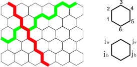
Figure 1: (Color online) Toric honeycomb lattice. The green loop (armchair) and the red loop (zig-zag) are two independent non-trivial loops.

II Toric honeycomb model

The model we propose is very simple. Consider a honeycomb lattice in a torus (See Fig. 1). The number of total sites is $2N$ and each site is occupied by a 1/2-spin. Define two plaquette operators

$$W_{P}=\sigma^{y}_{1}\sigma_{2}^{x}\sigma^{z}_{3}\sigma^{y}_{4}\sigma_{5}^{x}\sigma^{z}_{6},$$

$$\tilde{W}_{P}=\sigma^{x}_{1}\sigma_{2}^{y}\sigma^{z}_{3}\sigma^{x}_{4}\sigma_{5}^{y}\sigma^{z}_{6},$$ (1)

where 1, $\cdots$, 5, and 6 are the site indices of a plaquette $P$ as shown in Fig. 1. It is easy to directly check $W^{2}_{P}=\tilde{W}^{2}_{P}=1$, i.e, the eigenvalues of them are $\pm 1$; and $[W_{P},\tilde{W}_{P^{\prime}}]=0$ for all plaquette. The Hamiltonian is simply defined by sum over all plaquette

$$H=-J_{1}\sum_{P}W_{P}-J_{2}\sum_{P}\tilde{W}_{P},$$ (2)

where $J_{1}>0$ and $J_{2}>0$ and thus $W_{P}$ and $\tilde{W}_{P^{\prime}}$ are two-independent integrals of motion. This spin model is invariant in $x\,y\,z$ permutation. This model is exactly soluble: the ground states are given by the states with $W_{P}=\tilde{W}_{P}=1$ for all plaquette and the excited states are of at one plaquette having $W_{P}=-1$ or $\tilde{W}_{P}=-1$, which will be studied later in details.

III Ground states and degeneracy

The ground states are of the form

$$|G\rangle=\prod_{P}(1+W_{P})(1+\tilde{W}_{P})|\phi\rangle,$$ (3)

where $|\phi\rangle$ is an arbitrary reference state, e.g., $|\phi\rangle=|\uparrow\cdots\uparrow\rangle$ with each ‘$\uparrow$’ denoting the eigenvalue 1 of $\sigma^{z}_{i}$. The number of $|\phi\rangle$ is $2^{2N}$, the dimensions of the whole Hilbert space $\mathscr{H}$. The above construction of the ground states means the ground state space $L=\mathscr{H}/G$ where $G$ is the group generated by all independent $W_{P}$ and $\tilde{W}_{P}$. On the torus, due to the periodic boundary condition, there are two constraints $\prod_{P}W_{P}=\prod_{P}\tilde{W}_{P}=1$ for the generators, which means $G\cong(\mathbb{Z}_{2})^{2N-2}$. Therefore, according to the general theory given by Gottesman Go , the degeneracy of the ground states are $2^{2N-(2N-2)}=4$, which is exactly the same as that of the Kitaev toric code model kitaev .

One can even make a more intuitional proof similar to what Kitaev did kitaev . For a plaquette $P$, one defines $K_{ij}$ to be $\sigma^{z}_{i}\sigma_{j}^{z}$ for $(i,j)=(1,2),(4,5)$, $\sigma^{x}_{i}\sigma_{j}^{x}$ for $(i,j)=(2,3),(5,6)$, and $\sigma^{y}_{i}\sigma_{j}^{y}$ for $(i,j)=(3,4),(6,1)$; $\tilde{K}_{ij}$ to be $\sigma^{z}_{i}\sigma_{j}^{z}$ for $(i,j)=(1,2),(4,5)$, $\sigma^{y}_{i}\sigma_{j}^{y}$ for $(i,j)=(2,3),(5,6)$, and $\sigma^{x}_{i}\sigma_{j}^{x}$ for $(i,j)=(3,4),(6,1)$. For any closed loop, one can define two different operators

$$C=K_{ij}K_{jk}\cdots K_{si},~{}~{}\tilde{C}=\tilde{K}_{ij}\tilde{K}_{jk}\cdots\tilde{K}_{si}.$$ (4)

For any trivial loop on the torus, $C$ and $\tilde{C}$ are identical to the identity. There are only two unequivalent non-trivial loops as shown by the green and red in Fig. 1. Along the green loop, $C_{g}=\sigma^{y}_{i}\sigma^{y}_{j}\sigma_{k}^{z}\sigma^{z}_{l}\sigma^{y}_{m}\sigma^{y}_{n}\sigma_{s}^{z}\sigma^{z}_{t}\cdots$ and $\tilde{C}_{g}=\sigma^{x}_{i}\sigma^{x}_{j}\sigma_{k}^{z}\sigma^{z}_{l}\sigma^{x}_{m}\sigma^{x}_{n}\sigma_{s}^{z}\sigma^{z}_{t}\cdots$ while along the red loop, they are $C_{r}=\sigma^{x}_{i}\sigma^{x}_{j}\sigma_{k}^{x}\sigma^{x}_{l}\sigma^{x}_{m}\sigma^{x}_{n}\sigma_{s}^{x}\sigma^{x}_{t}\cdots$ and $\tilde{C}_{r}=\sigma^{y}_{i}\sigma^{y}_{j}\sigma_{k}^{y}\sigma^{y}_{l}\sigma^{y}_{m}\sigma^{y}_{n}\sigma_{s}^{y}\sigma^{y}_{t}\cdots$. These four operators generates all linear operators acting on the ground state space. In this way, we explicitly prove that the ground states are fourfold degenerate.

IV Low-lying excitations

IV.1 Excitations

Low-lying excitations of this exactly soluble model are given by

$$\sigma^{z}_{i_{b}}|G\rangle,$$

$$\psi_{i_{b}}|G\rangle=\sigma^{x}_{i_{b}}\prod_{i^{\prime}_{s}<i_{b}}\sigma^{z}_{i^{\prime}_{s}}|G\rangle,$$

$$\chi_{i_{b}}|G\rangle=\sigma^{y}_{i_{b}}\prod_{i^{\prime}_{s}<i_{b}}\sigma^{z}_{i^{\prime}_{s}}|G\rangle,$$

$$\sigma^{(1)}_{P}|G\rangle=\sigma^{z}_{i_{b}}\sigma^{z}_{i_{b}-2}\sigma^{z}_{i_{b}-4}\cdots|G\rangle,$$

$$\sigma^{(2)}_{P,P^{\prime}}|G\rangle=\sigma^{y}_{i_{b}}\sigma^{z}_{i_{b}-1}\sigma^{z}_{i_{b}-3}\cdots|G\rangle,$$

$$\sigma^{(3)}_{P,P^{\prime}}|G\rangle=\sigma^{x}_{i_{b}}\sigma^{z}_{i_{b}-1}\sigma^{z}_{i_{b}-3}\cdots|G\rangle,$$

$$\sigma^{(1)}_{P^{\prime}}|G\rangle=\sigma^{z}_{i_{b}-2}\sigma^{z}_{i_{b}-4}\sigma^{z}_{i_{b}-6}\cdots|G\rangle,$$ (5)

where the sites $i_{b}$ are shown in Fig. 1 and $P$ ($P^{\prime}$) label the plaquette where the site ’1’=$i_{b}$ ($i_{b}-2$); and the order of the sites is defined as follows: $i_{s}>j_{t}$ if the zig-zag line including $i_{s}$ is higher than that of $j_{t}$ or if $i_{s}$ is on the right hand of $j_{t}$ when they are in the same line. Except the first local excitation, all others are string-like excitations which are plotted in Fig.2.

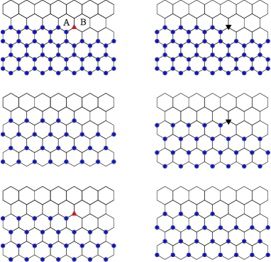
Figure 2: (Color online) The low-lying excitations. From left to right and up to down, they are $\psi_{i_{b}}$, $\chi_{i_{b}}$, $\sigma^{(1)}_{P}$, $\sigma^{(2)}_{P,P^{\prime}}$, $\sigma^{(3)}_{P,P^{\prime}}$, and $\sigma_{P^{\prime}}^{(1)}$. The up-triangles (red), down-triangles (black) and blue circles indicate acting the operators $\sigma^{x}$, $\sigma^{y}$ and $\sigma^{z}$ at these sites on the ground state, respectively.

Notice that $\sigma^{x}$, $\sigma^{y}$ and $\sigma^{z}$ anticommute with each other and therefore, if there is a red triangle ($\sigma^{x}$) or black triangle ($\sigma^{y}$) at site 3 or site 6 in a plaquette $P$, the eigenvalues of $W_{P}$ and $\tilde{W}_{P}$ of this plaquette become $-1$; if there is a blue circle ($\sigma^{z}$) at site 1, site 2, site 4 or site 5 in $P$, the eigenvalues of $W_{P}$ and $\tilde{W}_{P}$ of this plaquette also become $-1$; if there is a red triangle at site 1 or site 4, or a black triangle at site 2 or site 5, the eigenvalue of $W_{P}$ becomes $-1$; if there is a black triangle at site 1 or site 4, or a red triangle at site 2 or site 5, the eigenvalue of $\tilde{W}_{P}$ becomes $-1$. Taking $\psi_{i_{b}}$ as an example, the blue circle at site 1 in plaquette A (See Fig.2) makes the eigenvalues of $W_{A}$ and $\tilde{W}_{A}$ become $-1$, while the red triangle at site 5 makes the eigenvalue of $\tilde{W}_{A}$ become $-1$, and finally, the eigenvalue of $W_{A}$ in plaquette A becomes $-1$. For plaquette B, the red triangle at site 1 makes the eigenvalue of $W_{B}$ become $-1$. It is easy to check that the eigenvalues of $W$ and $\tilde{W}$ in other plaquette are not changed.

Although string-like excitations look like non-local , their energies are located at one or two sites. The energies of excitations can be calculated directly, which in turn are $4J_{1}$, $4J_{2}$, $4J_{1}+4J_{2}$ for $\psi,\chi,\sigma^{z}$ and $2J_{1}+2J_{2}$ for $\sigma^{(1,2,3)}$, respectively.

Notice that changing the subscript $i_{b}$ to $i_{w}$, the excitations do not change, i.e., we can redefine excitations as follows

$$\sigma^{z}_{i_{w}}|G\rangle,$$

$$\psi_{i_{w}}|G\rangle=\sigma^{y}_{i_{w}}\prod_{i^{\prime}_{s}<i_{w}}\sigma^{z}_{i^{\prime}_{s}}|G\rangle,$$

$$\chi_{i_{w}}|G\rangle=\sigma^{x}_{i_{w}}\prod_{i^{\prime}_{s}<i_{w}}\sigma^{z}_{i^{\prime}_{s}}|G\rangle,$$

$$\sigma^{(1)}_{P}|G\rangle=\sigma^{z}_{i_{w}}\sigma^{z}_{i_{w}-2}\sigma^{z}_{i_{w}-4}\cdots|G\rangle,$$

$$\sigma^{(2)}_{P,P^{\prime}}|G\rangle=\sigma^{x}_{i_{w}}\sigma^{z}_{i_{w}-1}\sigma^{z}_{i_{w}-3}\cdots|G\rangle,$$

$$\sigma^{(3)}_{P,P^{\prime}}|G\rangle=\sigma^{y}_{i_{w}}\sigma^{z}_{i_{w}-1}\sigma^{z}_{i_{w}-3}\cdots|G\rangle,$$

$$\sigma^{(1)}_{P^{\prime}}|G\rangle=\sigma^{z}_{i_{w}-2}\sigma^{z}_{i_{w}-4}\sigma^{z}_{i_{w}-6}\cdots|G\rangle.$$ (6)

The only difference is the interchange between $\sigma^{x}$ and $\sigma^{y}$, and it is easy to check excitations defined in Eqs. (IV.1) are the same as those in Eqs. (IV.1).

IV.2 Fusion Rules

All excitations are explicitly expressed by Pauli matrices. The fusion rules of these operators then can be directly calculated (See TABLE.1).

Table 1: Fusion rules of excitations.

	$\psi_{i_{b}}$	$\chi_{i_{b}}$	$\sigma^{z}_{i_{b}}$	$\sigma_{P}^{(1)}~{}$	$\sigma_{P,P^{\prime}}^{(2)}$	$\sigma_{P,P^{\prime}}^{(3)}$	$\sigma_{P^{\prime}}^{(1)}~{}$
$~{}\psi_{i_{b}}~{}~{}$	$~{}I~{}$	$i\sigma^{z}_{i_{b}}$	$-i\chi_{i_{b}}$	$-i\sigma_{P,P^{\prime}}^{(2)}$	$i\sigma_{P}^{(1)}~{}$	$\sigma_{P^{\prime}}^{(1)}~{}$	$\sigma_{P,P^{\prime}}^{(3)}$
$~{}\chi_{i_{b}}~{}~{}$	$-i\sigma^{z}_{i_{b}}$	$~{}I~{}$	$i\psi_{i_{b}}$	$i\sigma_{P,P^{\prime}}^{(3)}$	$\sigma_{P^{\prime}}^{(1)}~{}$	$-i\sigma_{P}^{(1)}~{}$	$\sigma_{P,P^{\prime}}^{(2)}$
$~{}\sigma_{i_{b}}^{z}~{}~{}$	$i\chi_{i_{b}}$	$-i\psi_{i_{b}}$	$~{}I~{}$	$\sigma_{P^{\prime}}^{(1)}$	$-i\sigma_{P,P^{\prime}}^{(3)}$	$i\sigma_{P,P^{\prime}}^{(2)}$	$\sigma_{P}^{(1)}$
$\sigma_{P}^{(1)}~{}$	$i\sigma_{P,P^{\prime}}^{(2)}$	$-i\sigma_{P,P^{\prime}}^{(3)}$	$\sigma_{P^{\prime}}^{(1)}$	$~{}I~{}~{}$	$-i\psi_{i_{b}}~{}~{}$	$i\chi_{i_{b}}~{}~{}$	$\sigma_{i_{b}}^{z}~{}~{}$
$~{}\sigma^{(2)}_{P,P^{\prime}}$	$-i\sigma_{P}^{(1)}$	$\sigma_{P^{\prime}}^{(1)}$	$i\sigma_{P,P^{\prime}}^{(3)}$	i$\psi_{i_{b}}$	$~{}I~{}~{}~{}$	$-i\sigma_{i_{b}}^{z}~{}~{}$	$\chi_{i_{b}}~{}~{}$
$~{}\sigma^{(3)}_{P,P^{\prime}}$	$\sigma_{P^{\prime}}^{(1)}$	$i\sigma_{P}^{(1)}$	$-i\sigma_{P,P^{\prime}}^{(2)}$	$-i\chi_{i_{b}}$	$i\sigma_{i_{b}}^{z}$	$~{}I~{}~{}~{}$	$\psi_{i_{b}}~{}~{}$
$~{}\sigma^{(1)}_{P^{\prime}}$	$\sigma_{P,P^{\prime}}^{(3)}$	$\sigma_{P,P^{\prime}}^{(2)}$	$\sigma_{P}^{(1)}$	$\sigma_{i_{b}}^{z}$	$\chi_{i_{b}}$	$\psi_{i_{b}}$	$~{}~{}I~{}~{}$

The fusion rules of the closed subset $\{I,\psi_{i_{b}},\sigma_{P}^{(1)},\sigma^{(2)}_{P,P^{\prime}}\}$ are exactly the same as the fusion rules in Kitaev toric code model if we identify $\psi,\sigma^{(1)}$ and $\sigma^{(2)}$ as $\varepsilon,e$ and $m$kitaev ; kitaev1 :

$$\psi^{2}=(\sigma^{(1)})^{2}=(\sigma^{(2)})^{2}=1,$$

$$\sigma^{(1)}\sigma^{(2)}=\psi,~{}~{}\psi\sigma^{(1)}=\sigma^{(2)},~{}~{}\sigma^{(2)}\psi=\sigma^{(1)}.$$ (7)

Here ‘= ’ may be up to a sign and/or ‘$i$’. Similarly, the subset $\{I,\chi_{i_{b}},\sigma_{P}^{(1)},\sigma^{(3)}_{P,P^{\prime}}\}$ also obeys the same fusion rules.

Because of the periodic boundary condition for a torus, the number of string-like excitations must be even.

V Braiding rules and anyons

Enlightened by this equivalence in the fusion rules, we check the braiding matrix. At first we find the statistics of the same kind excitations. It is easy to get $[\sigma^{(1)}_{P},\sigma^{(1)}_{P^{\prime}}]=0$, $[\sigma^{(2)}_{P_{1},P^{\prime}_{1}},\sigma^{(2)}_{P_{2},P^{\prime}_{2}}]=0$, and $\{\psi_{i_{b}},\psi_{j_{b}}\}=2\delta_{ij}$, i.e. $\sigma^{(1)}_{P}$ and $\sigma^{(2)}_{P,P^{\prime}}$ obey Bose statistics, while $\psi_{i_{b}}$ obey Fermi statistics. Since $\sigma^{(1)}\sigma^{(2)}=\psi$, the interchange between two $\psi$, $R_{\psi\psi}$, can be considered as product of $R_{\sigma^{(1)}\sigma^{(1)}}$, $R_{\sigma^{(2)}\sigma^{(2)}}$, $R_{\sigma^{(1)}\sigma^{(2)}}$ and $R_{\sigma^{(2)}\sigma^{(1)}}$, i.e.,note

$$R_{\psi\psi}=R_{\sigma^{(1)}\sigma^{(1)}}R_{\sigma^{(2)}\sigma^{(2)}}R_{\sigma^{(1)}\sigma^{(2)}}R_{\sigma^{(2)}\sigma^{(1)}}.$$ (8)

Clearly, $R_{\psi\psi}=-1$, $R_{\sigma^{(1)}\sigma^{(1)}}=1$ and $R_{\sigma^{(2)}\sigma^{(2)}}=1$, so $R_{\sigma^{(1)}\sigma^{(2)}}R_{\sigma^{(2)}\sigma^{(1)}}=-1$. This means when $\sigma^{(1)}$ circles around $\sigma^{(2)}$ or vice versa, a minus sign is acquired. In other words, they obey mutual semionic statistics. Braiding $\psi_{i_{b}}$ with $\sigma^{(1)}$ or $\sigma^{(2)}$ also gives $-1$. Similarly, statistics among $\chi_{i_{b}}$, $\sigma^{(1)}$ and $\sigma^{(3)}$ is also semionic.

VI Mapping to a square lattice

VI.1 Jordan-Wigner Transformation

This model can be mapped to a square lattice via a Jordan-Wigner transformation. For simplicity, we first restrict to the open boundary condition. We have defined $\psi_{i_{b}}$, $\chi_{i_{b}}$, $\psi_{i_{w}}$ and $\chi_{i_{w}}$ before. It is easy to check they are Hermitian and $\{\psi_{i_{b}},\psi_{j_{b}}\}=2\delta_{ij}$, $\{\psi_{i_{w}},\psi_{j_{w}}\}=2\delta_{ij}$ and $\{\psi_{i_{b}},\psi_{j_{w}}\}=0$. These relations are valid for $\chi$ as well. Furthermore, $\psi$ and $\chi$ are anticommutative. These operators can be thought as Majorana fermions, and can be combined into ’complex’ fermions

$$c^{{\dagger}}_{\uparrow,i}=\frac{1}{2}(\psi_{i_{w}}-i\psi_{i_{b}}),~{}~{}c_{\uparrow,i}=\frac{1}{2}(\psi_{i_{w}}+i\psi_{i_{b}}),$$

$$c^{{\dagger}}_{\downarrow,i}=\frac{1}{2}(\chi_{i_{w}}-i\chi_{i_{b}}),~{}~{}c_{\downarrow,i}=\frac{1}{2}(\chi_{i_{w}}+i\chi_{i_{b}}).$$ (9)

Expressing Pauli matrices by $\psi$ and $\chi$, we get

$$\sigma^{z}_{i_{w}}=-i\chi_{i_{w}}\psi_{i_{w}},~{}~{}\sigma^{z}_{i_{b}}=-i\psi_{i_{b}}\chi_{i_{b}},$$

$$\sigma^{y}_{i_{w}}=\psi_{i_{w}}\prod_{i^{\prime}_{s}<i_{w}}\sigma^{z}_{i^{\prime}_{s}},~{}~{}\sigma^{y}_{i_{b}}=\chi_{i_{b}}\prod_{i^{\prime}_{s}<i_{b}}\sigma^{z}_{i^{\prime}_{s}},$$

$$\sigma^{x}_{i_{w}}=\chi_{i_{w}}\prod_{i^{\prime}_{s}<i_{w}}\sigma^{z}_{i^{\prime}_{s}},~{}~{}\sigma^{x}_{i_{b}}=\psi_{i_{b}}\prod_{i^{\prime}_{s}<i_{b}}\sigma^{z}_{i^{\prime}_{s}}.$$ (10)

Thus, $W_{P}$ and $\tilde{W_{P}}$ can be expressed by $\psi$ and $\chi$ as

$$W_{P}=i\psi_{i_{w}}\psi_{i_{b}}i\psi_{j_{w}}\psi_{j_{b}},$$

$$\tilde{W_{P}}=i\chi_{i_{b}}\chi_{i_{w}}i\chi_{j_{b}}\chi_{j_{w}}.$$ (11)

Using the complex fermions, one has

$$W_{P}=(2n_{\uparrow,i}-1)(2n_{\uparrow,j}-1),$$

$$\tilde{W_{P}}=(2n_{\downarrow,i}-1)(2n_{\downarrow,j}-1),$$ (12)

where $n_{s,i}=c^{{\dagger}}_{s,i}c_{s,i}$ are the fermion number operators. The Hamiltion can be rewritten as

$$H=-J_{1}\sum_{\langle ij\rangle_{hd}}(2n_{\uparrow,i}-1)(2n_{\uparrow,j}-1)$$

$$-J_{2}\sum_{\langle ij\rangle_{hd}}(2n_{\downarrow,i}-1)(2n_{\downarrow,j}-1).$$ (13)

The symbol $\langle ij\rangle_{hd}$ means the sum is over nearest neighbors along the horizontal diagonals of squares (See Fig.3). In this way, we transfer the honeycomb lattice model to square lattice model composed of series of decoupled Ising chains as shown in Fig.3.

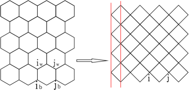
Figure 3: (Color online) Map from the honeycomb lattice to the square lattice. Ferromagnetic couplings are added to the two red lines.

VI.2 Ground states and Excitations

This square lattice model has been studied in our previous work yuli . The ground states of this Hamiltonian are $2^{M}$-fold degenerate, i.e., every individual chain is ferromagnetic, i.e., for a set of spins $\{s_{1},\cdots,s_{a},\cdots,s_{M}\}$,

$$|G_{\{s\}}\rangle=\prod_{a=1}^{M}|G_{s_{a}}\rangle=\prod_{a,i_{a}}c^{\dagger}_{s_{a},i_{a}}|0\rangle,$$ (14)

where $M$ is the number of chains, $i_{a}$ is the site index in the $a$-th chain. The low-lying excitations above a given ground state $|G_{\{s\}}\rangle$, for a given site $i_{a}$, reads

$${\cal H}_{i_{a}}|G_{\{s\}}\rangle = (c^{\dagger}_{s_{a},i_{a}}+c_{s_{a},i_{a}})|G_{\{s\}}\rangle=c_{s_{a},i_{a}}|G_{\{s\}}\rangle,$$

$${\cal D}_{i_{a}}|G_{\{s\}}\rangle = (c^{\dagger}_{\bar{s}_{a},i_{a}}+c_{\bar{s}_{a},i_{a}})|G_{\{s\}}\rangle=c^{\dagger}_{\bar{s}_{a},i_{a}}|G_{\{s\}}\rangle,$$

$${\cal F}_{i_{a}}|G_{\{s\}}\rangle = i{\cal H}_{i_{a}}{\cal D}_{i_{a}}|G_{\{s\}}\rangle=ic_{s_{a},i_{a}}c^{\dagger}_{\bar{s}_{a},i_{a}}|G_{\{s\}}\rangle,$$

$${\cal W}_{P}|G_{\{s\}}\rangle = \prod_{i^{\prime}_{b}\leq i_{a}}{\cal F}_{i^{\prime}_{b}}|G_{\{s\}}\rangle=\prod_{i^{\prime}_{b}\leq i_{a}}ic_{s_{b},i^{\prime}_{b}}c^{\dagger}_{\bar{s}_{b},i^{\prime}_{b}}|G_{\{s\}}\rangle,$$

$${\cal W}_{P,P^{\prime}}^{h}|G_{\{s\}}\rangle = \prod_{i^{\prime}_{b}<i_{a}}{\cal F}_{i^{\prime}_{b}}{\cal H}_{i_{a}}|G_{\{s\}}\rangle$$ (15)

$$= \prod_{i^{\prime}_{b}<i_{a}}ic_{s_{b},i^{\prime}_{b}}c^{\dagger}_{\bar{s}_{b},i^{\prime}_{b}}c_{s_{a},i_{a}}|G_{\{s\}}\rangle,$$

$${\cal W}_{P,P^{\prime}}^{d}|G_{\{s\}}\rangle = \prod_{i^{\prime}_{b}<i_{a}}{\cal F}_{i^{\prime}_{b}}{\cal D}_{i_{a}}|G_{\{s\}}\rangle$$

$$= \prod_{i^{\prime}_{b}<i_{a}}ic_{s_{b},i^{\prime}_{b}}c^{\dagger}_{\bar{s}_{b},i^{\prime}_{b}}c^{\dagger}_{\bar{s}_{a},i_{a}}|G_{\{s\}}\rangle,$$

where $P$ and $P^{\prime}$ denote two plaquette on the right and left of $i_{a}$, respectively. $\bar{s}=\downarrow(\uparrow)$ if $s=\uparrow(\downarrow)$. The order of sites is defined by $i^{\prime}_{b}<i_{a}$ if $i^{\prime}_{b}$ is on the left hand of $i_{a}$ for $b=a$ or $i^{\prime}_{b}$ is in a chain lower than the chain with $i_{a}$. ${\cal H,D,F}$ create a hole, a double occupant, and a spin-flip. ${\cal W}$, ${\cal W}^{d}$ and ${\cal W}^{h}$ create a half-infinite string of spin-flips, a spin-flip string with a double occupant and a spin-flip string with a hole, respectively, since the spins of fermions at sites $i^{\prime}_{b}<i_{a}$ are flipped from their ground state configuration while those at $j_{c}>i_{a}$ keep in their ground state configuration. These excitations are equivalent to those on honeycomb lattices with

$$\{{\cal H,D,F},{\cal W},{\cal W}^{h},{\cal W}^{d}\}\leftrightarrow\{\psi,\chi,\sigma^{z},\sigma^{(1)},\sigma^{(2)},\sigma^{(3)}\}.$$

VI.3 Equivalence in Low-lying Sector

As we have seen, the degeneracy of the ground states of the decoupled Ising chains is much higher than the toric honeycomb model. This means two models are not equivalent. This is caused by unproper treatment of the periodic boundary condition of the toric lattice in the Jordan-Wigner transformation. Due to the periodic boundary condition, an additional boundary Hamiltonian $H_{b}$ should be added to Eq. (13) yaok . The exact form of $H_{b}$ is complicated. Instead, we can use an approximation to deal with the periodic boundary condition so that the low-lying excitation sector is correct. We introduce Ising ferromagnetic boundary couplings to the system, i.e., for the two vertical red lines in Fig.3, we approximate the boundary effect from the Jordan-Wigner transformation through a boundary coupling Hamiltonian

$$H_{b}=-g_{1}\sum_{\langle ij\rangle_{1};s}n_{is}n_{js}-g_{2}\sum_{\langle ij\rangle_{2};s}n_{is}n_{js}~{},$$ (16)

where $1$ and $2$ label two vertical red lines in Fig.3 and $\langle ij\rangle_{1,2}$ mean the sum is over corresponding vertical lines. We assume $g_{1,2}$ is much larger than $J_{1,2}$, the energy scale of the low-lying excitations, so that the opposite nearest neighbor spins along a given boundary line do not create additional low-lying excitations. Clearly, this kind of couplings make all odd/even chains have the same states in a given ground state. Therefore, the degeneracy of the ground states is the same as two decoupled Ising chains, i.e., 4. And couplings will not change the ground state. Due to the periodic boundary condition, low-lying excitations will appear in pairs. Thus, as long as excitations do not cross the vertical boundary lines, excitations are low-lying . The statistics of excitations in square lattice are the same as those in honeycomb lattice, see yuli .

VII Conclusions

We have constructed a toric honeycomb model and proved that it is equivalent to Kitaev toric code model in square lattice. This honeycomb model is helpful to understand the toric code of anyons in a more symmetric way. It was also shown that this model can be mapped into an Ising chain array with boundary couplings, which proposed a possible realization of the anyon models in a conventional interacting fermion model.

We thank Yi Li for useful discussions and the contribution in the early stage of this work. This work was supported by National Natural Science Foundation of China, the national program for basic research of MOST of China, the Key Lab of Frontiers in Theoretical Physics of CAS and a fund from CAS.

References

- (1) A. Kitaev, Ann. Phys. 303, 2(2003).
- (2) J. M. Leinaas and J. Myrheim, Nuovo Cimento 37 B, 1 (1977).
- (3) F. Wilczek, Phys. Rev. Lett. 48, 1144 (1982).
- (4) R. B. Laughlin, Phys. Rev. Lett. 50, 1395 (1983).
- (5) R. De Picciotto, M. Reznikov, M. Heiblum, V. Umansky, G. Bunin, and D. Mahalu, Nature 389, 162 (1997).
- (6) L. Saminadayar, D. C. Glattli, Y. Jin, and B. Etienne, Phys. Rev. Lett. 79, 2526 (1997).
- (7) D. Arovas, J. R. Schrieffer and F. Wilczek, Phys. Rev. Lett. 53, 722 (1983).
- (8) F. E. Camino, W. Zhou and V. J. Goldman, Phys. Rev. B 72, 075342 (2005).
- (9) G. Moore and N. Read, Nucl. Phys. B 360, 362 (1991).
- (10) N. Read and E. Rezayi, Phys. Rev. B 59, 8084 (1999).
- (11) M. H. Freedman, M. J. Larsen, and Z. Wang, Commun. Math. Phys. 227, 605 (2002).
- (12) L. Fu and C. L. Kane, Phys. Rev. Lett. 100, 096407 (2008); Phys. Rev. Lett. 102, 216403 (2009).
- (13) M. A. Levin and X.-G. Wen, Phys. Rev. B 71, 045110 (2005)
- (14) A. Kitaev, Ann. Phys. 321, 2(2006).
- (15) Y.-J. Han, R. Raussendorf and L.-M. Duan, Phys. Rev. Lett. 98, 150404 (2007). C. -Y. Lu, W. -B. Gao, O. Gühne, X. -Q. Zhou, Z. -B. Chen, and J. -W. Pan, Phys. Rev. Lett. 102, 030502 (2009). J. K. Pachos, W. Wieczorek, C. Schmid, N. Kiesel, R. Pohlner, and H. Weinfurter, New J. Phys. 11, 083010 (2009).. L. Jiang, G. K. Brennen, A. V. Gorshkov, K. Hammerer, M. Hafezi, E. Demler, M. D. Lukin, and P. Zoller, Nature Physics 4, 482 (2008). J. -F. Du,. J. Zhu, M. -G. Hu, and J. -L. Chen, arXiv:0712.2694. M. Aguado, G. K. Brennen, F. Verstraete, and J. I. Cirac, Phys. Rev. Lett. 101, 260501 (2008). B. Paredes and I. Bloch, Phys. Rev. A 77, 023603 (2008).
- (16) C. Zhang, V. W. Scarola, S. Tewari and S. Das Sarma, Proc. Natl. Acad. Sci. U.S.A. 104, 18415 (2007). K. P. Schmidt, S. Dusuel and J. Vidal, Phys. Rev. Lett. 100, 057208 (2008); J. Vidal, S. Dusuel and K. P. Schmidt, Phys. Rev. Lett. 100, 177204 (2008).
- (17) V. Lahtinen, G. Kells, A. Carollo, T. Stitt, J. Vala and J. K. Pachos, Ann. of Physics 323, 2286 (2008).
- (18) Y. Yu and Y. Li, J. Phys. A: Math. Theor. 43, 105306 (2010).
- (19) H. Yao and S. A. Kivelson, Phys. Rev. Lett. 99, 247203 (2007).
- (20) D. Gottesman, Phys. Rev. A 54, 1862 (1996).
- (21) To have a graphic understanding for this relation, see Fig. 4 in yuli .