Optimization of transport protocols with path-length constraints in complex networks

Abstract

We propose a protocol optimization technique that is applicable to both weighted or unweighted graphs. Our aim is to explore by how much a small variation around the Shortest Path or Optimal Path protocols can enhance protocol performance. Such an optimization strategy can be necessary because even though some protocols can achieve very high traffic tolerance levels, this is commonly done by enlarging the path-lengths, which may jeopardize scalability. We use ideas borrowed from Extremal Optimization to guide our algorithm, which proves to be an effective technique. Our method exploits the degeneracy of the paths or their close-weight alternatives, which significantly improves the scalability of the protocols in comparison to Shortest Paths or Optimal Paths protocols, keeping at the same time almost intact the length or weight of the paths. This characteristic ensures that the optimized routing protocols are composed of paths that are quick to traverse, avoiding negative effects in data communication due to path-length increases that can become specially relevant when information losses are present.

I Introduction

Communication systems are an essential element of the modern world, and represent some of the most noticeable settings of transport problems in complex structures. The Internet, telephone systems, power grids, etc., provide ways to transport information, signals or resources from one part of the globe to another. Such communication is done by means of highly structured systems that can be modeled by networks, i.e., collections of elements corresponding to nodes, links that interconnect them, and weights on the links symbolizing connection capabilities albertrev ; newmanrev ; sergeibook ; romubook ; alainbook .

In many examples of communication systems, discrete subsets of information (packets) are sent from a source to the appropriate destination. Typically, a multitude of users simultaneously perform similar tasks between many different source-destinations pairs, and thus the network at any given time is populated by numerous traveling data packets. In order for packets to find their way, routing protocols are put in place which determine how the packets travel from source to destination. Optimization of the performance in communication systems can thus be achieved in two non-exclusive ways: improving the structure of transport networks guimera02 , and finding optimal routing protocols ohira98 . Both approaches have been the focus of a great deal of research on this subject in recent years guimera02 ; ohira98 ; arenas01 ; sole01 ; echenique04 ; echenique05 ; lopez06 ; braunstein07 ; Cohen ; LPP ; braunstein03 ; goh01 ; marc03 ; sree04 ; sree06 ; danila06 ; danila07 ; yan00 ; kalisky05 ; goh05 . A number of important results have been obtained, elucidating the usefulness of so-called scale-free networks guimera02 ; lopez06 , the vulnerability of networks to random or targeted failures of some of its elements Cohen , and the relevance of path-lengths in the efficiency of communication LPP .

When the overall traffic in the network is very large, the system may get compromised in its capability to deliver information. The origin of this problem could be twofold: either the connections of the network are unable to tolerate such a high traffic flow or, more commonly, some components (nodes) get overloaded, i.e., congested. Congestion occurs when the nodes become heavily used acting as bottlenecks for the network communication. By establishing clever routing protocols, this congestion can be diminished or, for moderate rates of overall traffic in the system, eliminated. The assessment of node work-load requires thus the introduction of a new quantity. Betweenness centrality (betweenness in short) has been proposed as such a measure guimera02 ; goh01 , as an estimate of how much use a given node can expect to receive. Specifically, for a set of paths in a network, the betweenness of a node is defined as the number of paths visiting that node. Therefore, a given routing protocol induces a betweenness on the nodes of the network. It has been pointed out that nodes with large betweenness are the first to form packet queues when traffic is large enough guimera02 . If this queue is not eliminated, then the travel times of packets from source to destination increase without bound, hence, rendering the node (and potentially the network) congested.

On the other hand, packet delivery is an imperfect process since it can be subjected to packet loss or corruption. When congestion occurs, even entire queues of packets could be eliminated while waiting at overloaded nodes. Thus, when attempting to optimize a routing protocol, care must be taken not to increase the path-length to a level that would elevate the likelihood of packet loss beyond critical limits. Such considerations have led to the formulation of models such as Limited Path Percolation, which exhibit a phase transition when the length of paths increases beyond a specific tolerance level LPP .

In this article, we focus on the problem of optimizing the transport rules for scale-free networks with properties similar to those of computer networks. However, in contrast to a number of other studies, we optimize the protocols to reduce the likelihood of congestion but keeping path-lengths as close as possible to the shortest, thus guaranteeing efficient communication paths. We find that by applying ideas borrowed from Extremal Optimization (EO) boett01 , which uses local information to approach the optimal state of a system, we can achieve both goals of congestion avoidance and short path-lengths.

The article is structured as follows: Sec. II explains the philosophy behind our optimization heuristic, the algorithm to find optimal routing protocols, and our network model. Sec. III quantifies betweenness of nodes as a consequence of the optimized routing protocol. Sec. IV focuses on the path-lengths created by the new, EO-based, routing protocol, and the advantages that it affords regarding maintaining the path-lengths within a constant factor of the original paths. Sec. V extends our methods to weighted networks, and finally, Sec. VI is dedicated to the conclusions.

II Optimization method

To define the betweenness precisely, we need first to specify a routing protocol, which is a set of paths $\mathcal{L}=\{\rho_{ij}\}$ between all pairs of nodes $i$ and $j$ of the network. We define the length of each path $\ell_{ij}$ as the minimum number of links needed to be crossed when going from $i$ to $j$ following the path $\rho_{ij}$. We adhere to the convention of considering only one path for each pair of nodes sree06 , as the length degeneracy of the paths will be exploited by the method to optimize the protocol. The rules by which these paths are chosen can be numerous. For instance, one typical choice for $\mathcal{L}$ in the literature is the set of shortest paths between nodes (SP). The betweenness $b_{i}$ of a node $i$ is then defined as the number of paths of $\mathcal{L}$ that visit node $i$, without counting those paths that begin or end in $i$. (This choice is somewhat arbitrary, and other choices are also possible.) Note that in the literature the word ”betweenness” sometimes is associated exclusively with the number of paths crossing a node within the framework of the SP protocol. We are using this concept in a more general context since it can refer to any routing protocol, which has to be given. In fact, betweenness values depend on both, the structure of the network and $\mathcal{L}$. For a given network, changing the routing protocol typically changes ${b_{i}}$ over the network except in very special cases such as when there is only one possible protocol choice (e.g., a star network).

Given a network and a protocol $\mathcal{L}$, it has been shown that the first node to begin accumulating a queue, say $m$, satisfies that $b_{m}>b_{i}$ for all nodes $i\neq m$ in the network guimera02 . To explain this point, consider a network of size $N$ in which data packets are produced in each node at random with a rate $0\leq\gamma\leq 1$. In the simplest version of the problem, the destination of each packet is random too, and thus, each node can produce a packet to any of the other $N-1$ nodes of the network with equal probability. In this case, it was found that the number of packets in node $i$ is, on average, $\gamma\,b_{i}/(N-1)$ guimera02 . Without loss of generality, we assume that each node can processes (route through) a single packet per unit time, and thus, the first node to congest is the one with the maximum betweenness value, $b_{\rm max}$. We can also rephrase this point by indicating that the critical rate of packet production would be $\gamma_{c}=(N-1)/b_{\rm max}$ before some node of the network congests guimera02 . This relation shows the relevance of designing routing protocols with a $b_{\rm max}$ as low as possible in order to prevent network congestion for low $\gamma$ values. The lower $b_{\rm max}$ is, the higher the number of packets can be (higher $\gamma$) before the network congests. There is, however, a price to pay in this strategy because the reduction of $b_{\rm max}$ is usually attained at the expense of enlarging the path-lengths. Under some circumstances, such as when packets can get lost, enlarging significantly the paths may not be the best option. The model that we propose next aims at bridging the gap between these two opposing forces: we explore how much $b_{\rm max}$ can be reduced while keeping the paths as close to their shortest version as possible.

We generate the networks for the analysis with the configuration model  reed-molloy95 ; romu05 that allows us to build graphs with arbitrary degree sequence but free from degree-degree correlations. The degree of a node $i$ corresponds to its number of connections and is usually represented as $k_{i}$. In this work, we will focus on power-law degree distributed networks, $P(k)\sim k^{-\lambda}$, with exponent $\lambda=2.5$ to facilitate the comparison with previous studies sree06 ; danila06 ; yan00 . Nevertheless, we have also performed the analysis on networks with $\lambda=4.5$ finding no qualitative difference in the final results.

The optimization algorithm starts from the SP protocol: Once the network is built, the first step is to calculate the shortest paths between all nodes of the network using Dijkstra’s algorithm cormen . Then, in an iterative way for as long as desired, we repeat the following steps:

• The node with the highest betweenness $m$ is selected.

• One of the paths, $\rho_{ij}$, passing through $m$ is chosen at random; we refer to its initial and final nodes as $i$ and $j$ (with $i\neq m\neq j$).

• A path between $i$ and $j$ is searched. The new path must be the shortest alternative to $\rho_{ij}$ not passing through $m$. In case that there are more than one alternative paths degenerate in length, one of them is selected at random. On the other hand, if there is no alternative to $\rho_{ij}$, the path remains without change.

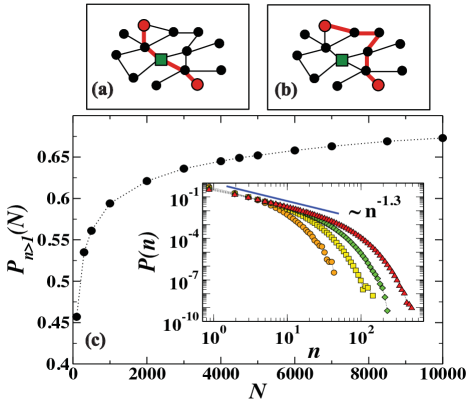
Figure 1: (Color Online) The sketches (a) and (b) illustrate the way in which the method optimizes the protocol by selecting another path that must be either of the same length or the shortest alternative to the original one. In panel (c), the probability of finding alternative length-degenerate paths, $P_{n>1}$, for the Shortest-Path protocol is displayed as a function of the network size $N$. In the inset: histogram for the number $n$ of degenerate alternatives for each path in the SP protocol. The different curves correspond to the following network sizes: $N=100$ (circles), $500$ (squares), $2000$ (diamonds) and $10000$ (triangles).

A schematic illustration of these rules is shown in panels (a) and (b) of Figure 1. In the sketch, a path passing through the highest betweenness node, the square, is re-routed thereby reducing betweenness. It is worth stressing that, the constraint on the length of the alternative paths in practice means that if another choice of equal length to the original path exists, the path does not increase in length. The method takes advantage of the possible degeneracy of the paths with respect to length to change the protocol and ease the stress on the node(s) with the largest traffic. Note also that the method keeps no long-term memory, the search for alternative paths due to sequential expulsions of a path from different nodes do not accumulate. The algorithm generates thus protocols with paths limited to SP configurations or the shortest alternatives to them avoiding a single high used node.

The potential utility of exploiting the SP degeneracy and its importance in our networks can be seen in Figure 1. We have plotted in the panel (c) the probability of finding a degenerate alternative to the shortest path between any pair of nodes $i$ and $j$, $P_{n>1}(N)$, as a function of the network size $N$. $P_{n>1}(N)$ consistently grows with $N$, becoming higher than $65\%$ for the largest graphs that we have considered $N=10000$. In the inset, the distribution of the number of different degenerate paths, $P(n)$, is also shown for four network sizes. Note that $P_{n>1}=\sum_{n=2}^{\infty}P(n)$.

The philosophy of our method is in the spirit of Extremal Optimization (EO) boett01 , attacking the worst element of the system in an attempt to improve the global performance. In the following, we will study how its application affects the different features of the protocols.

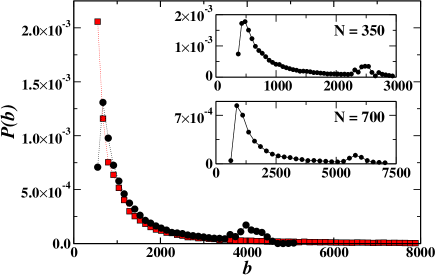
Figure 2: (Color Online) Betweenness distribution for a $N=500$ system. The (black) circles correspond to the stationary distribution reached with our optimization method while the (red) squares are for the initial SP protocol. In the inset, the stationary betweenness distributions of the method for other two network sizes: $N=350$ and $N=700$.

III Betweenness distribution

We will discuss first the results concerning the betweenness of the nodes and how its values adapt after the optimization method is employed. After some iterations of the method stat the betweenness distribution, $P(b)$, reaches a stationary form that can be seen in Figure 2. Before describing it, it is important to remember that the SP protocol produces a power-law distribution for $P(b)$ whose exponent depends on the exponent $\lambda$ of the degree distribution goh01 ; marc03 (see the curve of (red) squares in Figure 2). The protocols generated by the optimization method show that the tail of $P(b)$ collapses into a peak at high values of the betweenness. Also the area of low $b$ suffers a slight variation, although the functional form of $P(b)$ at intermediate $b$ seems largely unaffected. A change in the size of the network displaces the position of the peak but not the quality of the effects observed in the main plot of Figure 2.

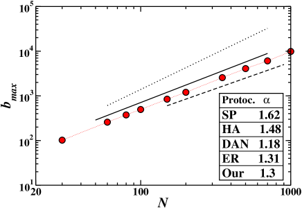
Figure 3: (Color Online) The average maximum betweenness, $b_{max}$, as a function of the network size $N$ for the optimized protocols. Lines are shown as a reference scaling with exponent $1.3$ (solid), $1.18$ (dashed), and $1.62$ (dotted). In the table, scaling exponents $\alpha$ obtained with different optimization methods are listed. The initials correspond to Shortest-Paths (SP) yu07 , Hub-Avoidance (HA) sree06 , Danila’s method (DAN) danila06 , Efficient Routing (ER) yan00 , and our own method.

The peak induced in $P(b)$ by the optimization method at high values of $b$ correlates with a decline of the maximum betweenness in the network. As mentioned before, this betweenness, $b_{max}$, is of crucial importance for the transport capability of a protocol, since it imposes an upper cutoff to the traffic that the network is able to sustain before congesting guimera02 ; braunstein07 . The scaling of $b_{max}$ with the network size, $N$, can thus be seen as a measure of the scalability of a routing protocol: the faster $b_{max}$ grows with $N$, the less useful the protocol is for large networks. In Figure 3, the average $b_{max}$ in the stationary state of the protocols obtained with our optimization method is depicted as a function of the number of nodes in the network. We find a power-law increase with a functional form $b_{max}\sim N^{\alpha}$ and $\alpha^{our}\approx 1.3$. This value of $\alpha$ must be compared with the results encountered with other protocols or other protocol optimization methods. In the same Figure, we have also included a table with the exponents $\alpha$ for other methods. It is specially interesting to compare with the original Shortest-Path protocol $\alpha^{SP}\approx 1.62$ yu07 or with the best of the optimization methods listed (Danila’s method) with $\alpha^{DAN}\approx 1.18$ danila06 ; danila07 . Our optimization method, without deviating substantially from the SP protocol in the length of the paths, produces an acceptable value of the exponent $\alpha$.

IV Path-Lengths

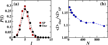
Figure 4: (Color Online) In panel (a), path-length distribution for a network of size $N=1000$. In the figure, the results of the protocols obtained with our optimization method can be compared with the initial SP. In panel (b), the ratio between the average length of the paths in the two protocols (ours and SP) is visualized as a function of the network size.

The near-invariance of the path-length between SP and our optimized protocol, and the path-length distribution itself, deserves further attention. Here we will focus on studying how the length of the paths in the protocol mutates when the optimization method is applied to the protocol. In Figure 4, we have plotted the path-length distribution $P(\ell)$ for the original Shortest Path protocol (red squares) and for the stationary regime of the protocols obtained with our optimization method on a network of size $N=1000$. As can be seen, the distribution is slightly displaced to larger values of $\ell$ but its shape remains essentially invariant. In order to quantify the relevance of the change of $P(\ell)$ with the system size, we have represented in panel (b) of Figure 4 the ratio between the average length of the paths in the protocols obtained with our method and that calculated with the SP. The curve is monotonically decreasing with $N$, moving very slowly towards unity (or a value just above).

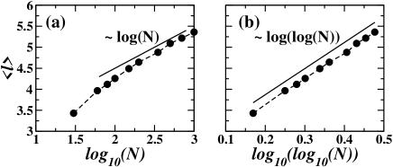
Figure 5: Average path-length, $\langle l\rangle$, of the protocols we obtain as a function of the network size. It can be seen that a $log(log())$-scale in panel (b) provides a better fit to our simulation results than a pure logarithmic scale in (a).

Similar to $b_{max}$, limiting the scaling of the average length of the paths, $\langle\ell\rangle$, with the system size is also an important design feature. A protocol that elongates the paths unnecessarily may not be efficient for network communications. Generally, there exists a nonzero probability of losing a packet in every communication between two servers, and the longer the paths become, the higher the probability of missing information. Furthermore, if data loss reaches a point in which most of the paths are not functioning, the network suffers a disruption similar to a percolation transition. In fact, this phenomenon has been studied recently and it is known as Limited Path Percolation LPP . In Figure 5, we show how $\langle\ell\rangle$ in the protocols obtained using our method behaves with increasing network sizes. In scale-free networks with $\lambda=2.5$, the SP protocol $\langle\ell_{SP}\rangle$ is expected to grow as $\log({\log({N})})$. We cannot numerically test this formula for many decades in $N$ for our optimized protocols, but within the limited range of values that we can explore the relation holds. Such scaling is important because, as mentioned above, the optimization of the protocols can in some cases imply a trade-off between reductions in $b_{max}$ and escalating path-lengths. For instance, Danila’s method danila06 , which exhibits the best scaling for $b_{max}$ versus $N$ of the methods shown in Figure 3, leads to a $\langle\ell\rangle\sim\log({N})$ danila07 , considerably faster than the $\log({\log({N})})$-scaling of our method (or of the SP protocol). This difference in the scaling can be relevant if the packet communication has losses in long paths (or in paths longer than the SP).

In general, consider a protocol that is tuned to scale with the typical structural path lengths of the network, which, to be concrete, we associate with the most probable length $\ell_{SP}^{*}$ of the length distribution $P_{SP}(\ell)$. We imagine that the real system uses a protocol $\mathcal{L}_{o}$ when uncongested which is, for our purposes, the best practical protocol for the network of interest (even if it is not strictly optimal). For a power-law network with exponent $\lambda=2.5$, $\ell^{*}_{o}=D_{o}\ell^{*}_{SP}\sim D_{o}\log\log(N)$, where $D_{o}\geq 1$ is a numerical constant. Now, when higher rates of packet creation appear on the network, to avoid congestion we consider introducing two new protocols $\mathcal{L}_{S}$ and $\mathcal{L}_{L}$, the first one with typical path lengths $\ell^{*}_{S}\sim\delta_{S}\ell^{*}_{o}$ ($\delta_{S}>1$ another constant), and the second with $\ell^{*}_{L}=F(\ell^{*}_{o})$, with $F(x)>x^{1+\epsilon}$, $\epsilon>0$. In the thermodynamic limit, with mean field approximation, $\tau$, the ratio of new typical path length to old typical path length in $\mathcal{L}_{S}$ remains constant, as we can see from

$$\tau_{S}=\frac{\ell^{*}_{S}}{\ell^{*}_{o}}=\frac{\delta_{S}D_{o}\log\log(N)}{D_{o}\log\log(N)}\rightarrow\delta_{S}.$$ (1)

On the other hand, for $\mathcal{L}_{L}$, we find

$$\tau_{L}=\frac{F(D_{o}\log\log(N))}{D_{o}\log\log(N)}\rightarrow(D_{o}\log\log(N))^{\epsilon}\rightarrow\infty$$ (2)

where the last relation occurs for $N\rightarrow\infty$. In Ref. LPP , the limited path percolation transition was shown to be intimately related to $\tau$. For our purposes, it means that if a protocol keeps $\tau$ finite as $N\rightarrow\infty$, occurring in the $\tau_{S}$ case, there is the possibility to have a protocol that can be tuned to maintain at least a level of communication between node pairs. Note that the $\mathcal{L}_{S}$ protocol can be written as $F(x)=x$. On the other hand, if $\tau$ diverges, as in $\tau_{L}$, as the system size grows, the typical pair of nodes becomes increasingly distant in the relative sense, and thus cannot in general remain in communication, or in a more formal sense, protocols such as $\mathcal{L}_{L}$ may not be scalable fn_Fx .

The protocol we propose here has the behavior of $\mathcal{L}_{S}$ and thus, as in limited path percolation, can have a percolation threshold to a connected regime. Furthermore, the fact that we study scale-free degree distributed networks with small $\lambda$ indicates that from the standpoint of limited path percolation, there is always a connected regime. In addition, when $\delta$ is close to 1, that the protocol is very robust as most pairs of nodes remain connected after the introduction of the optimization of $b_{max}$. These conclusions are also supported by results displayed in Figures 4, 5 and 6.

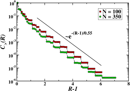
Figure 6: Color Online) Cumulative distribution of the ratio between the length of the paths obtained with our protocol optimization method and those of the corresponding original SP. The distribution becomes step-like due to the discreteness of the length.

Furthermore, as explained above, a path obtained with our method can be only in two states: either the SP configuration or, if they were expelled from a high used node and no length-degenerate alternative was available, in the shortest configuration that does not pass through that node. Such two state configuration recalls physical systems in which the components can be in the energetic ground state or being activated by thermal (stochastic) fluctuations to higher energy levels. To confirm whether this parallelism is valid, we have plotted in Figure 6 the cumulative distribution ($C_{>}(R)=\int_{R}^{\infty}dR^{\prime}\,P(R^{\prime})$) of the ratios $R=\ell_{stat}/\ell_{SP}$, where $\ell_{stat}$ corresponds to the length of each path in an stationary instance of the protocols obtained with our optimization technique and $\ell_{SP}$ is the corresponding length of the shortest path. As can be seen, the probability for the paths to be outside the ground state (SP), in an ”excited state”, decays as an exponential function with a characteristic ratio that depends on the graph (whether the graph is scale-free or not, and, if it is, also on the exponent of the degree distribution). In the example of Figure 6, the characteristic ratio is around $1.55$, which makes it extremely unlikely for any path to suffer a large stretching out of its SP length. This exponential decaying $C_{>}(R)$ resembles the Boltzmann factor in which $R-1$ plays the role of the energy.

V Weighted networks

The introduction of disorder in the network connections deeply modifies the previous scenario. However, connections of divers quality can be expected in may real-world situations. A classical example within the context of transport is the Internet and the variability on bandwidth of the connections between servers. Mathematically speaking, the quality of a connection can be represented by a scalar attached to each link that is known as its weight $w$. The presence of weighted links alters the definition of shortest path park ; newman01 ; newman04 . Instead of ”short” in the sense of number of links between origin and destination, it may be important to find the path with the lowest weight along the way (or the largest, depending on the quality that the weight conveys). These paths are often referred to as optimal paths in the literature (see, for instance, cieplak ).

Protocols based on Optimal Paths (OP) also have a very particular scaling with the network size braunstein07 . Depending on the level of randomness on the weights of the connections, the system can fall into a strong- or a weak-disorder regime. The difference between these two regimes is that in the strong-disorder case the fluctuations on the weight are so large that the accumulated weight along each paths is controlled by the edge with the highest weight, while in weak-disorder the ”responsibility” for the path’s overall weight is distributed among all the links along the path wu ; chen . In the two regimes, the scaling of $b_{max}$, and of the average weight of the paths $\langle w_{path}\rangle$, with $N$ changes with respect to unweighted graphs goh05 . Here we will focus only on the weak-disorder regime since it is the only one in which it makes sense to search for an alternative protocol to the OP. The cost of doing so in the strong-disorder limit would diverge with the size of the graph.

One of the positive aspects of our protocol optimization is that its generalization to weighted graphs is straightforward: at each step, a path passing through the node with the highest betweenness is chosen to be redirected. The path is then exchanged by its alternative of lowest cost that does not pass through that node. As before, if there is no alternative, the path remains invariant. In the following, we will study the performance of the stationary protocols produced by this method on Molloy-Reed graphs with $\lambda=2.5$ and with two possible functional forms for the weight distributions: either an exponential $P(w)\sim e^{-w/w_{c}}$ or a power-law $P(w)\sim w^{-\beta}$. In order to keep the results comparable for both distributions, we fix the parameter $w_{c}$ to obtain a similar average weight as in the power-law distribution. For the data shown, this will be $w_{c}=2$ and $\beta=2.5$.

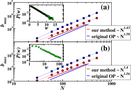
Figure 7: (Color Online) Dependence of $b_{max}$ with the system size for weighted graphs. The (red) circles are the results for the protocols of our method and the (blue) squares are for the original OP protocol. The weight distribution in panel (a) follows an exponential $P(w)\sim e^{-w/2}$, and in (b) the power-law $P(w)\sim w^{-2.5}$, as displayed in the insets for networks of size $N=500$. The continuous curves in both panels are a guide to the eye showing a visual comparison between the exponent values obtained by fitting the simulation results.

The scaling of $b_{max}$ as a function of the network size is shown in Figure 7 for networks with both type of weight distributions. The application of the optimization method produces a significant improvement in $b_{max}$ with respect to the Optimal Paths protocol. For the range of system sizes of the figure, this entails an improvement by a factor $3$ or even higher. Additionally, the exponent $\alpha$ of the optimized protocols is close to $1.4$ while that of the original OP protocols was about $1.55$. One can wonder about the price to pay for such an improvement. In networks with continuous values of the weights, any degeneracy in the weight of the alternative paths is extremely unlikely. Strictly speaking, then, there is always a price to pay, although it could be minute. To answer this question, we have plotted in Figure 8 the average weight of the paths scaled with $N$ for protocols obtained with our method and for the corresponding OP on both types of networks and both weight distributions. Similarly to the unweighted case, we find that the average weight is slightly higher but not extremely so. Also the ratio between the average weight of the paths of our optimized protocols and of OP decreases for increasing network sizes. Furthermore, even though it is not shown in the figure, neither the shape of the distribution nor the weight of the paths is hardly altered by the optimization of the protocols.

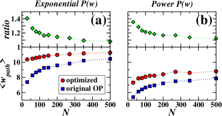
Figure 8: (Color Online) Comparison between the average weight of the paths, $\langle w_{path}\rangle$, in the original OP protocol and in the optimized protocols with our method. The curves in (a) correspond to weighted graphs with an exponentially decaying weight distribution, while those in (b) have a power-law weight distribution.

VI Discussion and Conclusion

We study a routing protocol optimization method that takes advantage of the degeneracy of the shortest paths to reduce the congestion in the nodes of the network. The paths between node pairs in the optimized protocols can only be in two states: they can be either one of the shortest-paths or the closest alternative avoiding highly used nodes. We use ideas coming from Extremal Optimization to guide our algorithm, which proves to be an effective technique. The resulting routing protocols show an appreciable reduction of the maximum node betweenness, $b_{\rm max}$, while keeping the path-length distribution similar to the lower bound provided by the SP protocol. For the networks that we have analyzed $b_{\rm max}$ increases with $N$ as a power-law with an exponent $\alpha\approx 1.3$. That is only slightly higher than the best values reported in the literature, and, in contrast to those methods, the average path-length appears to retain the $\log{(\log{(N)})}$-scaling of the SP protocol. We show that methods which do not conserve a constant ratio of path-length with the topological shortest paths end up in a disconnected phase of percolation with limited paths, which is a possible indicator that on networks with packet loss such methods may not be scalable.

Our method is easily generalized for weighted networks. We have studied two examples of weighted networks in the weak-disorder regime and found significant reductions in $b_{\rm max}$ with respect to the Optimal Paths protocol as well as in the scaling exponent with which $b_{\rm max}$ grows with $N$.

As we implemented the optimization method–a procedure in which we keep record of all the paths passing through each node–, the numerical performance is not optimal. Indeed, we were able to study a range of network sizes wide enough to characterize the scaling of the optimized protocols properties, but not as large as to allow for large network analysis. Our aim in this work was to explore the behavior of the optimization method and to ascertain whether the resulting routing protocols have interesting features concerning the size scaling and behavior of $b_{\rm max}$ and the path-length distributions. Indeed, the simple fact that we have shown that it is feasible to perform such dual optimization is an important step forward. Furthermore, we have found that this two parameter optimization is important because without taking into account both $b_{max}$ and path-length, the protocols that simply reduce $b_{max}$ may be less scalable.

Therefore, the possibility of searching for efficient numerical methods to implement the optimization algorithm remains open for future work. A possible solution, depending on the structure of the network, can be the implementation of a local search technique for the alternative paths. This local method could be highly efficient if the clustering (the density of triangles) in the graph is high as typically occurs in geographically embedded or social driven networks. Locally tree-like structured networks, such as those considered here, typically require global rearrangements between paths of nearly-degenerate length but hardly any overlap, as illustrated by Fig. 1a-b. Maintaining the paths of the routing protocol short can be crucial in situations such as when the system suffers packet losses, a circumstance that seems to be relatively frequent in practice. Our optimization method represents in such cases a useful tool that offers a balance between betweenness reduction (lower congestion) and restricted path-lengths (reduced losses) in routing protocols.

VII Acknowledgments

EL acknowledges funding from the EPSRC grant EPSRC EP/E056997/1. JJR is funded by the FET grant 233847-Dynanets of the EU Commission. Also both JJR and SB acknowledge support by the U. S. National Science Foundation through grant DMR-0312510.

References

- (1) R. Albert A-. L. Barabási, Rev. Mod. Phys. 74, 47 (2002).
- (2) M. E. J. Newman, SIAM Rev. 45, 167 (2003).
- (3) S. Dorogovtsev and JFF Mendes, Evolution of Networks: From Biological Nets to the Internet and WWW, Oxford University Press (2003).
- (4) R. Pastor-Satorras and A. Vespignani, Evolution and structure of the Internet : a statistical physics approach, Cambridge University Press (2004).
- (5) A. Barrat, M. Barthélemy and A. Vespignani, Dynamical Processes on Complex Networks, Cambridge University Press (2008).
- (6) R. Guimerà, A. Díaz-Guilera, F. Vega-Redondo, A. Cabrales and A. Arenas, Phys. Rev. Lett. 89, 248701 (2002).
- (7) T. Ohira, and R. Sawatari, Phys. Rev. E. 58, 193 (1998).
- (8) A. Arenas, A. Díaz-Guilera, and R. Guimera, Phys. Rev. Lett. 86, 3196 (2001).
- (9) R.V. Solé and S. Valverde, Physica A. 289, 595 (2001).
- (10) P. Echenique, J. Gómez-Gardeñes and Y. Moreno, Phys. Rev. E. 70, 056105 (2004).
- (11) P. Echenique, J. Gómez-Gardeñes and Y. Moreno, Europhys. Lett. 71, 325 (2005).
- (12) E. López, S. Carmi, S. Havlin, S.V. Buldyrev and H.E. Stanley, Physica D 224, 69 (2006).
- (13) L.A. Braunstein et al., International Journal of Bifurcation and Chaos 17, 2215 (2007).
- (14) R. Cohen, K. Erez, D. ben-Avraham and S. Havlin, Phys. Rev. Lett. 86, 3682 (2001).
- (15) E. López, R. Parshani, R. Cohen, S. Carmi and S. Havlin, Phys. Rev. Lett. 99, 188701 (2007).
- (16) L.A. Braunstein, S.V. Buldyrev, R. Cohen, S. Havlin and H.E. Stanley, Phys. Rev. Lett. 91, 168701 (2003).
- (17) K.-I. Goh., B. Kahng and D. Kim, Phys. Rev. Lett. 87, 278701 (2001).
- (18) M. Barthélemy, Phys. Rev. Lett. 91, 189803 (2003).
- (19) S. Sreenivasan, T. Kalisky, L.A. Braunstein, S.V. Buldyrev, S. Havlin and H.E. Stanley, Phys. Rev E 70, 046133 (2004)
- (20) S. Sreenivasan, R. Cohen, E. López, Z. Toroczkai, and H. E. Stanley, Phys. Rev. E 75, 036105 (2007).
- (21) B. Danila, Y. Yu, J.A. Marsh and K. E. Bassler, Phys. Rev. E 74, 046106 (2006)
- (22) B. Danila, Y. Yu, J.A. Marsh and K. E. Bassler, Chaos 17, 036102 (2007).
- (23) G. Yan, T. Zhou, B. Hu, Z.-Q. Fu and B.H. Wang, Phys. Rev. E. 73, 046108 (2006).
- (24) T. Kalisky, L.A. Braunstein, S.V. Buldyrev, S. Havlin and H.E. Stanley, Phys. Rev. E. 72, 025102(R) (2005).
- (25) K.-I. Goh, J.D. Noh, B. Kahng and D. Kim, Phys. Rev E 72, 017102 (2005).
- (26) S. Boettcher and A.G. Percus, Phys. Rev. Lett. 86, 5211 (2001); Artificial Intelligence 119, 275 (2000).
- (27) M. Molloy and B. Reed, Random Structures and Algorithms 6, 161 (1995).
- (28) M. Catanzaro, M. Boguñá and R. Pastor-Satorras, Phys. Rev. E 71, 027103 (2005).
- (29) T.H. Cormen, C.E. Leiserson, R.L. Rivest and C. Stein, Introduction to Algorithms, McGraw-Hill (2005).
- (30) As a criterion to define the stationarity of the optimization process, we focus on the value of as a function of the iteration steps. is considered over the last 20 steps, and the process is said stationary if the relative error . We confirmed the stationary of the betweenness and path-length distributions within numerical precision once this criterion is fulfilled. The number of path rearrangements required to achieve stationary protocols scales for the networks studied approximately as .
- (31) Y. Yu, B. Danila, J.A. Marsh and K.E. Bassler, Europhys. Lett. 79, 48004 (2007).
- (32) K. Park, Y-. C. Lai, and N. Ye, Phys. Rev. E 70, 026109 (2004).
- (33) M.E.J. Newman, Phys. Rev. E. 64, 016132 (2001).
- (34) M.E.J. Newman and M. Girvan, Phys. Rev. E. 69, 026113 (2004).
- (35) M. Cieplak, A. Maritan, and J. R. Banavar, Phys. Rev. Lett. 72, 2320 (1994).
- (36) Y. Chen, E. López, S. Havlin, and H. E. Stanley, Phys. Rev. Lett. 96, 068702 (2006).
- (37) Z. Wu, E. López, S. V. Buldyrev, L. A. Braunstein, S. Havlin, and H. E. Stanley, Phys. Rev. E 71, 045101(R) (2005).
- (38) Note that any function scaling faster than and diverging is sufficient to obtain the same qualitative results. For instance, has the same effect. In general, if the paths scale too fast for a protocol satisfying limited paths to be scalable.