Quasiregular mappings of polynomial type in
Abstract
Complex dynamics deals with the iteration of holomorphic functions. As is well-known, the first functions to be studied which gave non-trivial dynamics were quadratic polynomials, which produced beautiful computer generated pictures of Julia sets and the Mandelbrot set. In the same spirit, this article aims to study the dynamics of the simplest non-trivial quasiregular mappings. These are mappings in which are a composition of a quadratic polynomial and an affine stretch.
MSC2010: 30C65 (Primary), 30D05, 37F10, 37F45 (Secondary)
1 Introduction
The field of complex dynamics, the study of iteration of analytic functions in the plane, goes back nearly a century to Fatou and Julia. However, there has been a surge of recent interest in the field, following on from computer generated pictures of Julia sets and the Mandelbrot set and led by the work of Douady and Hubbard, e.g. [5]. This illustrated how an iterative system with a very simple description, namely a quadratic polynomial, could have very complicated behaviour. There are several excellent introductions to the theory, for example [1, 11, 12].
More recently, the iteration of quasiregular mappings in has been studied, motivated by the fact that several key tools in complex dynamics have analogues for quasiregular mappings, for example Rickman’s theorem generalizing Picard’s theorem, and Montel’s theorem. In fact, direct analogues of the Fatou and Julia sets can be defined for a special class of quasiregular mappings, all of whose iterates have distortion bounded by some fixed number. These are the so-called uniformly quasiregular mappings, introduced in [9] and studied in a number of papers. We restrict ourselves to mentioning [8] and the interested reader can find further references contained therein.
For general quasiregular mappings, it is no longer possible to define the Fatou set for the simple reason that the iterates will have no common bound on the distortion (see the standard references [13, 10] for the theory of quasiregular mappings). It is however possible to define the escaping set , the set of those points which iterate to infinity, which is a key object in complex dynamics. It is well known that for an analytic function, the boundary of coincides with the Julia set. It is therefore natural to consider for quasiregular mappings and see to what extent it can be considered an analogue of the Julia set. Recent papers in this direction include [2, 3, 4].
Of particular relevance here is [7], where it was shown that for quasiregular mappings of polynomial type, as long as the degree of the mapping is larger than the distortion, is an infinite, completely invariant perfect set. Further, the family of iterates of is not equicontinuous at any point of .
In this paper, in the same spirit as the study of iteration of quadratic polynomials, we aim to analyze the boundary of the escaping set for the simplest quasiregular mappings with non-trivial dynamics; namely the composition of quadratic polynomials and quasiconformal mappings with constant complex dilatation.
The outline of the paper is as follows. In section 2, we will cover some preliminary definitions and results. In section 3, a canonical form for the type of functions we are interested in will be derived. In section 4, generalizations of results in [7], on the boundary of the escaping set, to our functions will be obtained. Section 5 deals with the connectedness or not of , and section 6 introduces a generalization of the Mandelbrot set and covers some of its properties.
The images in this paper were computed using the Python programming language and the NumPy (Numerical Python) extension package. The code is available on the second authors’ website http://thesamovar.net/mathematics/qrdynamics.
The authors would like to thank Dan Nicks for interesting and stimulating discussions.
2 Preliminaries
We first collect some definitions and results that we will use. A quasiregular mapping from a domain is called quasiregular if belongs to the Sobolev space and there exists such that
| (2.1) |
almost everywhere in . Here denotes the Jacobian determinant of at . The smallest constant for which (2.1) holds is called the outer distortion of . If is quasiregular, then we also have
| (2.2) |
almost everywhere in for some . The smallest constant for which (2.2) holds is called the inner distortion of . The maximal distortion of is the larger of and . In dimension , we have .
The degree of a mapping is the maximal number of pre-images and is in direct analogue with the degree of a polynomial. A quasiregular mapping is said to be of polynomial type if its degree is uniformly bounded at every point, or equivalently, if as .
Theorem 2.1 ([7]).
Let and be -quasiregular of polynomial type. If the degree of is greater than the inner distortion , then is a non-empty open set and is perfect.
Denote by the branch set of , that is, the set where is not locally injective. A quasiconformal mapping is an injective quasiregular mapping. The following result says that in dimension , a quasiregular mapping can be factorized into two mappings, one of which deals with the distortion and one which deals with the branch points.
Theorem 2.2 (Stoilow factorization, see for example [10] p.254).
Let be a quasiregular mapping. Then there exists an analytic function and a quasiconformal mapping such that .
Stoilow factorization tells us what the branch set of a quasiregular mapping in can be.
Corollary 2.3.
Let be quasiregular. Then is a discrete set of points. In particular, if is quasiregular of polynomial type, then is a finite set of points.
3 Canonical form
It is well-known that every quadratic polynomial is linearly conjugate to for an appropriate . We will find an analogous canonical form for compositions of quadratic polynomials and affine stretches.
Consider a quasiconformal mapping which stretches by a factor in the direction . If , then . For general , pre-compose by a rotation of and post-compose by a rotation of to give the expression
| (3.1) |
or
| (3.2) |
Using the formula for complex dilatation (see [6]), we see that
| (3.3) |
and so which means that is quasiconformal with constant complex dilatation. Solving the Beltrami equation (see [6]) with the complex dilatation of (3.3) gives a quasiconformal map which is unique if we require the solution the fix three points. Therefore given and , the unique solution of the Beltrami equation with dilatation (3.3) which fixes and is the stretch given by (3.1).
Given a stretch , we will represent it as a point in , given by the point . Note that a stretch of factor in any direction is just the identity.
Proposition 3.1.
Let be a composition of a quadratic polynomial and an affine stretch of the form (3.1). Then is linearly conjugate to
| (3.4) |
for some and . Moreover, if we insist that , where
| (3.5) |
then such a representation is unique.
Proof.
Let be a quadratic polynomial, where with , let for and , and write . We need to know how behaves under pre-composition by translations and dilations. Let for . Then using (3.2),
| (3.6) |
Let for . Again using (3.2), and noting that is -linear,
| (3.7) |
Using (3.6) with ,
Applying (3.7) with ,
Therefore is linearly conjugate to (3.4) with , and .
For the uniqueness, we note that the choice of and for a given constant complex dilatation (3.3) is not unique. There are the obvious symmetries and . These correspond to the facts that a stretch in a direction is the same as stretching in the direction , and that stretching a factor in the direction is the same, up to post-composing by a conformal dilation, as stretching by a factor in the perpendicular direction. That is, and . There are no other such symmetries.
We see that is linearly conjugate to via the conjugation . So if , then we can apply such a conjugation (and take if necessary) so that .
Recalling that all stretches with are identical, we see that if we require , then the canonical form for is unique. ∎
For brevity, we will define the set
We will also mention the set
and so .
We observe that the dynamics of in Proposition 3.1 correspond to those of , in particular, if and only if . Therefore, every composition of a quadratic polynomial and an affine stretch is linearly conjugate to some element of , and so we just need to study the dynamics of mappings in .
4 The boundary of the escaping set
The escaping set is defined as
Recalling Theorem 2.1, the requirement that the distortion is smaller than the degree is a necessary one as the following example shows.
Example 4.1.
Consider the winding map in polar coordinates. This map decomposes as where and . The partial derivatives of are
and so the complex dilatation is
We conclude that and the distortion of is . Therefore the distortion of is , and clearly the degree of is , but is empty, since for every .
Therefore, Theorem 2.1 only applies to those with by (3.3). However, in our special situation, we can actually deduce the results of Theorem 2.1 by modifying the proof. For , write , where and for and . We first estimate the growth of .
Lemma 4.2.
Let be as above and set . Then for any ,
Further, is -bi-Lipschitz, that is
for all .
Proof.
This follows immediately from the definition of , since
where and . The fact that is bi-Lipschitz follows from the -linearity of . ∎
We extend Theorem 2.1 in dimension as follows.
Theorem 4.3.
Let be a polynomial of degree and let be -bi-Lipschitz. Let , then is a non-empty open set and is a perfect set.
Proof.
A bi-Lipschitz mapping is quasiconformal, and so is quasiregular. The first step is to show that is non-empty. Since is -bi-Lipschitz and for large , we have
Therefore there exists such that
for , and we can conclude that this neighbourhood of infinity is contained in . The openness of follows from the continuity of quasiregular mappings and the fact that contains a neighbourhood of infinity. Clearly is completely invariant, and therefore is completely invariant.
The fact the is open means that has no isolated points. To show that is perfect, we therefore have to show that has no isolated points. This is the part of the proof that requires modification when compared to Theorem 2.1. Exactly as in the proof of that theorem (we omit the details here, see [7]), we assume for contradiction that if is an isolated point of , and see that then .
Since , we must have , where is the local index. Therefore
Using again the fact that is bi-Lipschitz,
for . nd so there is a neighbourhood of which is not in , giving a contradiction. ∎
We remark that in the Stoilow decomposition of the function in Example 4.1, it is easy to see that the quasiconformal mapping is not bi-Lipschitz.
Corollary 4.4.
Let . Then is a non-empty open set, and is a perfect set.
The following theorem is proved in [7], and the proof goes through exactly as there and so is omitted.
Theorem 4.5.
Let be as in Theorem 4.3. Then for any , . The family of iterates is equicontinuous on and not equicontinuous at any point of . The set is infinite. The sets , and are all completely invariant. The escaping set is a connected neighbourhood of infinity.
In particular, we have the conclusions of Theorem 4.5 for . One may be tempted to ask whether the proof that is perfect goes through as soon as contains a neighbourhood of infinity. A modification of the winding map shows that this is not the case.
Example 4.6.
For and with , define . This mapping decomposes as where and . We can calculate that the distortion of this mapping is , that every point except escapes, and so . Clearly is not a perfect set. We note that is not bi-Lipschitz.
5 Connectedness of
Let be quasiregular of polynomial type and either the distortion of is smaller than the degree or . Then we define the set of points whose orbits remain bounded
Clearly and is completely invariant by Theorem 4.5. This set is the direct analogue of the filled-in Julia set for polynomials, but here we are reserving the use of the symbol for distortion.
Recall the branch set is the set where is not locally injective. In this section, we will give proofs for , but the proofs will work equally well for or when the degree of is larger than the distortion. We first need a quasiregular version of the Riemann-Hurwitz formula.
Theorem 5.1 (Riemann-Hurwitz formula).
Let be domains in whose boundaries consist of a finite number of simple closed curves. Let be a proper holomorphic map of onto with branch points including multiplicity. Then every has the same number of pre-images including multiplicity and
| (5.1) |
where is the number of boundary components of .
Corollary 5.2.
The Riemann-Hurwitz formula (5.1) holds when is a quasiregular mapping of degree in .
Proof.
By Theorem 2.2, we can write , where is holomorphic and is quasiconformal. Since is quasiconformal, it does not alter the number of boundary components of , has no branch points in and every has exactly one pre-image under in . Therefore every has pre-images under in including multiplicity, has branch points including multiplicity in and so we can apply (5.1) to . ∎
We now move on to our first connectedness result.
Theorem 5.3.
Let . Then is connected if and only if .
Proof.
Recall from the proof of Theorem 4.4 the existence of a neighbourhood of infinity contained in .
First assume that . Then gives a quasiregular -sheeted covering of onto with no branching, since has degree . Since is simply connected, so is every . Since , then must be simply connected and hence is connected.
Conversely, suppose that is not empty. Let be the smallest value of such that is not empty. Applying Corollary 5.2 to the quasiregular map
with , and , we see that . This implies that is not simply connected and hence is not connected. ∎
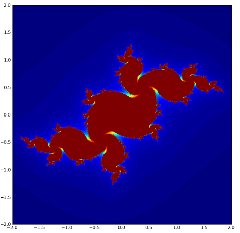
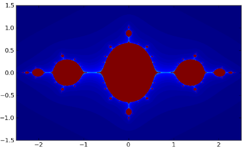
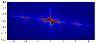
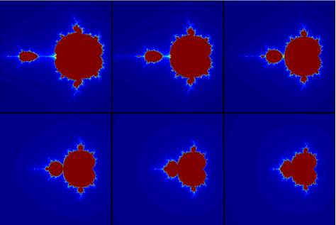
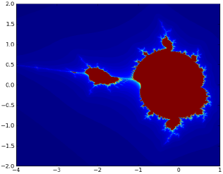
Since is the only branch point of , this theorem is only interested in whether escapes or not. However, we have formulated it this way, because the proof is equally valid for or when the degree of is larger than the distortion, both cases where may have more than one branch point. Examples of connected are the Douady dragon of Figure 1, the pinched basilica of Figure 2 and the banking airplane of Figure 3.
Moving back to the case , if is not connected, then the following result tells us that is actually infinitely connected.
Theorem 5.4.
Let . If contains , then is infinitely connected.
Proof.
Since , the forward orbit of ,
accumulates only at infinity. Hence there exists a simple closed curve such that the interior of contains and the exterior contains . Since is a neighbourhood of infinity and contained in ,
and hence there exists such that . This implies that has single valued locally injective quasiregular branches on , denoted by for .
Then the sets are pairwise disjoint, and we call this collection of sets . Each is compactly contained in and contains images for , and we denote the collection of such sets over all by . One can inductively define the collection for every , and by construction,
Since , we see that is infinitely connected. ∎
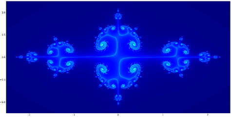
For quadratic polynomials, if contains , then is totally disconnected, i.e. every connected component is a point. This is not necessarily the case for , as suggested by Figure 4 for and , where each connected component appears to be a continuum. One can check that by using the condition in Theorem 6.3 below, and so really is disconnected, by Theorem 5.4, as claimed.
6 Parameter space
For each pair such that , we can consider the parameter space obtained by varying over functions in . We are led to the following definition.
Definition 6.1.
Let , and with decomposition where and for . The -Mandelbrot set is defined be the set of those for which .
Theorem 6.2.
We have the following characterisation of :
Proof.
As is well-known, the Mandelbrot set is contained in the disk . We will show that the -Mandelbrot set is also a bounded set.
Theorem 6.3.
Let . Then
where . Further, is compact and can be characterised as the set of for which for all .
Proof.
Fix such that , and recall from Lemma 4.2 that satisfies for all , where . Assume that . Then and
For , assume that
Then
when . Therefore, by induction, and is not in the -Mandelbrot set.
For the second part of the theorem, assume that
for some and . First note if then . So if , then
| (6.1) |
If , then and (6.1) implies that . Therefore by induction,
and we can conclude that and so . On the other hand, if , then and (6.1) implies that and so by induction,
and again . This argument shows that the complement of is open and so itself is a compact set. ∎
See Figure 5 for various Mandelbrot sets with . It may appear that a bulb is detached from the main cardioid for , but the following theorem shows that, among other things, these two components of are attached by a segment contained in . See also Figure 6 for this effect.
Theorem 6.4.
If , then
If , then there exists an angle and a real number such that the line segment
for
Proof.
If , and , then for all . It is well-known that , i.e. does not escape under iteration of only when . Since for , then this observation implies that
For the second part, assume that , and set and . Clearly maps rays emanating from to other such rays and has obvious fixed rays. We first show that , which also maps rays to rays, has at least one fixed ray too.
One can calculate that is given, in polar coordinates, by
| (6.2) |
For , write for the ray . Then it is easy to see that maps the ray onto , where
| (6.3) |
To show that has a fixed ray, we therefore need to find a solution to . Rearranging (6.3), this means we need to solve
| (6.4) |
Let . Then (6.4) and the addition formula for the tangent function yield
Rearranging this equation, we need to find a zero of the cubic polynomial
Every cubic with real coefficients has a real zero, and we claim that has a zero in . To see this, note that and . Since , we have and the claim follows. Therefore, with
fixes . Using (6.2), we see that acts on the fixed ray by
The final claim of the theorem follows with
by using the same argument from the first part of the theorem. We remark that if , then and , agreeing with the first part of the theorem. ∎
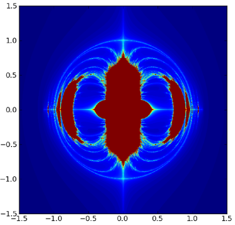
We remark that the parameter space for mappings in is actually two complex dimensional, since we have a different mapping for each pair . Denote by the set of such that is bounded. Each -Mandelbrot set is a one dimensional slice of this larger parameter space . Similarly, one can consider one dimensional slices of where is fixed, and varies. As an example, Figure 7 is the slice of through . Note the expected rotational symmetry. Further, the slice is the whole of . A natural question to ask is whether the set is connected in , just as the Mandelbrot set is connected in the parameter space of quadratic polynomials?
References
- [1] A. F. Beardon, Iteration of rational functions, Graduate Texts in Mathematics, 132, Springer-Verlag, New York, 1991.
- [2] W. Bergweiler Karpinska’s paradox in dimension three, to appear in Duke Math. J.
- [3] W. Bergweiler, A. Eremenko, Dynamics of a higher dimensional analog of the trigonometric functions, preprint.
- [4] W. Bergweiler, A. Fletcher, J. Langley, J. Meyer, The escaping set of a quasiregular mapping, Proc. Amer. Math. Soc., 137, no.2, 641-651, 2009.
- [5] A.Douady, J.H.Hubbard, It ration des polyn mes quadratiques complexes [Iteration of complex quadratic polynomials], C. R. Acad. Sci. Paris S r. I Math., 294, no. 3, 123–126 (1982).
- [6] A.Fletcher, V.Markovic, Quasiconformal maps and Teichmüller theory, OUP, 2007.
- [7] A.Fletcher, D.A.Nicks, Quasiregular dynamics on the n-sphere, to appear in Ergodic Theory and Dynamical Systems.
- [8] A. Hinkkanen, G. Martin, V. Mayer, Local dynamics of uniformly quasiregular mappings, Math. Scand., 95, no. 1, 80-100, 2004.
- [9] T. Iwaniec, G. Martin, Quasiregular semigroups, Ann. Acad. Sci. Fenn., 21, no. 2, 241–254, 1996.
- [10] T. Iwaniec, G. Martin, Geometric function theory and non-linear analysis, Oxford Mathematical Monographs, Oxford University Press, New York, 2001.
- [11] J. Milnor, Dynamics in one complex variable, Third edition, Annals of Mathematics Studies, 160, Princeton University Press, Princeton, NJ, 2006.
- [12] S.Morosawa, Y.Nishimura, M.Taniguchi and T.Ueda, Holomorphic dynamics, CUP, 2000.
- [13] S. Rickman, Quasiregular mappings, Ergebnisse der Mathematik und ihrer Grenzgebiete 26, Springer, 1993.
Institute of Mathematics, University of Warwick, Coventry, CV4 7AL, UK.
Email address: alastair.fletcher@warwick.ac.uk
Equipe Audition, Département d’Etudes Cognitives, Ecole Normale Supérieure, 29 Rue d’Ulm,
75230, Paris, Cedex 05.
Email address: dan.goodman@ens.fr