A generalized multiple-try version of the Reversible Jump algorithm

Abstract

The Reversible Jump algorithm is one of the most widely used Markov chain Monte Carlo algorithms for Bayesian estimation and model selection. A generalized multiple-try version of this algorithm is proposed. The algorithm is based on drawing several proposals at each step and randomly choosing one of them on the basis of weights (selection probabilities) that may be arbitrary chosen. Among the possible choices, a method is employed which is based on selection probabilities depending on a quadratic approximation of the posterior distribution. Moreover, the implementation of the proposed algorithm for challenging model selection problems, in which the quadratic approximation is not feasible, is considered. The resulting algorithm leads to a gain in efficiency with respect to the Reversible Jump algorithm, and also in terms of computational effort. The performance of this approach is illustrated for real examples involving a logistic regression model and a latent class model.
Keywords: Bayesian inference, Latent class model, Logistic model, Markov chain Monte Carlo, Metropolis-Hastings algorithm.

1 Introduction

Markov chain Monte Carlo (MCMC) methods have had a profound impact on Bayesian inference. In variable dimension problems, which mainly arise in the context of Bayesian model selection, a well-known approach is the Reversible Jump (RJ) algorithm proposed by Green (1995). The algorithm uses the Metropolis-Hastings (MH) paradigm (Metropolis et al., 1953; Hastings, 1970) in order to generate a reversible Markov chain which jumps between models with different parameter space dimensions. These jumps are achieved by proposing a move to a different model, and accepting it with appropriate probability in order to ensure that the chain has the required stationary distribution. However, the algorithm presents some potential drawbacks that may limit its applicability. Ideally, the proposed moves are designed so that the different models are adequately explored. However, the efficient construction of these moves may be difficult because, in general, there is no natural way to choose jump proposals (see, among others, Green, 2003).

Several approaches have been proposed in literature in order to improve the efficiency of the RJ algorithm. An interesting modification of the MH algorithm is the Delayed Rejection (DR) method, proposed by Tierney and Mira (1999) and extended to the RJ setting by Green and Mira (2001). The method is based on a modified between-model move, conditional on the rejection of the initial trial. In particular, if a proposal is rejected, a second move is attempted and it is accepted with a probability that takes into account the rejected first proposal, in a way that satisfy the detailed balance condition. Obviously, the efficiency improvements of the two-stage proposal needs to be weighed against the increased computational cost.

Moreover, Brooks et al. (2003) proposed two main classes of methods. The first class explores the idea to automatically scale the parameters of the jump proposal distribution by examining a Taylor series expansion of the Hastings ratio as a function of the parameters of the proposal distribution. The broad idea is that first and second order (and possibly higher order) terms in the Taylor expansion are set equal to zero, giving a system of equations that are solved to yield the optimal proposal parameters. The rationale for doing this is that it should lead to higher acceptance probabilities, thereby improving the ability of the sampler to move between models. However, for many statistical models, generating such a Taylor expansion and solving first and second derivatives is analytically unavailable, as is the case of the latent class (LC) model considered in this paper. The second approach proposed in Brooks et al. (2003), termed the saturated space approach, develops the idea of augmenting the state space with auxiliary variables (to ensure that all models have the same dimension as the largest one) in order to allow the chain to have the same memory of the states visited in other models, increasing the efficiency of the proposals.

Other approaches include the automatic RJ sampler by Hastie (2005). This approach requires a pilot run for each model under consideration in order to learn about the posterior distribution within each model. This information is then used inside a RJ algorithm to tune proposal parameters when jumping between models. Clearly this comes at a high computational cost, particularly when the model dimension is large. In a similar vein, Lunn et al. (2009) developed an inferential framework in which the BUGS software (Spiegelhalter et al., 1996) can be used to carry out RJ inference. The main constraint here is that the full-conditional distributions for the parameters are available in closed form within each model. Moreover, Fan et al. (2009) approached the issue of constructing proposals for between model moves by estimating particular marginal densities based on MCMC draws from the posterior, using path sampling. In more detail, suppose that the parameter vectors within the models can be partitioned so that a subset of them can be held constant when moving between models. When a between model move is proposed, the new parameters are drawn from a proposal distribution which is conditioned upon the subset of previously sampled parameters. The main computational burden is to actually draw from this conditional distribution, especially when the parameter space is high dimensional. This is the major drawback of the approach of Fan et al. (2009). Furthermore, note that population MCMC, whereby a target distribution is constructed consisting of a product of tempered versions of the target distribution of interest, has also been developed for RJ (Jasra et al., 2007). The idea here is that the collection of states of the population of the Markov chain at any given iteration can be used to give some guidance for selecting parameters of the proposal distribution. But also the effect of tempering is to allow efficient exploration of a potentially multi-modal target distribution. The main drawback is that only one particular Markov chain in the population (with temperature equal to $1$) is used for inferential purposes. The remaining chains serve to facilitate mixing within and between models. Finally, another interesting approach was proposed by Bartolucci et al. (2006), which consists of employing in a more efficient way the output of an RJ algorithm implemented in the usual way in order to construct a class of efficient estimators of the Bayes factor. For a review of the main methodological extensions of the RJ algorithm see also Fan and Sisson (2011) and Hastie and Green (2012).

With the aim of improving the performance of the RJ algorithm, in this paper we extend the results illustrated in Pandolfi et al. (2010) in which a generalization of the Multiple-Try Metropolis (MTM) algorithm of Liu et al. (2000) is proposed in the context of Bayesian estimation and Bayesian model choice. In particular we develop their idea of applying a multiple-try strategy to increase the efficiency of the RJ algorithm from a Bayesian model selection perspective, where the dimensionality of the parameter space is also part of the model uncertainty.

In general, the MTM algorithm represents an extension of the MH algorithm consisting of drawing, at each step, a certain number of trial proposals and then selecting one of them with a suitable probability. The selection probabilities of each proposed value are constrained so as to attain the detailed balance condition. In particular, Liu et al. (2000) proposed a rule to choose these probabilities so that they are proportional to the product of the target, the proposal, and a function which is non-negative and symmetric. The generalization of the multiple-try scheme proposed by Pandolfi et al. (2010), hereafter denoted by GMTM, defines the selection probabilities in a more general way. Under this approach, minimal constraints are required to attain the detailed balance condition. In principle, any mathematical function giving valid probabilities may be adopted to select among the proposed trials although the efficiency in the estimation of the target distribution may depend on this choice.

In the Bayesian model choice context, the GMTM extension of the RJ algorithm represents a rather natural way to overcome some of the typical problems of this algorithm, as for example the necessity of an accurate tuning of the jump proposals. The extension consists of proposing, at each step, a fixed number of moves, so as to promote mixing among models. In particular, among the possible ways to compute the selection probabilities, we suggest a method based on a quadratic approximation of the target distribution that may lead to a considerable saving of computing time. Moreover, we show that, when it is not possible to easily compute this quadratic approximation, the generalized version may again lead to an efficient algorithm. It is also worth noting that the proposed extension of the RJ algorithm has several analogies with the DR method of Green and Mira (2001), in which the different trial proposals are attempted only conditionally to the rejection of the first one. Given these similarities, this method may be easily adapted for a direct comparison with the proposed approach, as we illustrate in this paper.

The remainder of the article is structured as follows. In Section 2 we review the MH algorithm and the RJ algorithm and we introduce the basic concept of the GMTM algorithm for Bayesian estimation. In Section 3 we outline the generalized multiple-try version of the RJ algorithm with a discussion on some convenient choices of the selection probabilities. The proposed approach is illustrated in Section 4 by some empirical experiments, whereas Section 5 provides main conclusions.

2 Preliminaries

We first introduce some basic notation for the MH and the RJ algorithms and we briefly review the GMTM method as a generalization of the MTM algorithm.

2.1 Metropolis-Hastings and Reversible Jump algorithms

The MH algorithm, proposed by Metropolis et al. (1953) and modified by Hastings (1970), is one of the best known MCMC method to generate a random sample from a target distribution $\pi(\mbox{\boldmath$\theta$})$. The basic idea of this algorithm is to construct an ergodic Markov chain in the state space of $\theta$ that has $\pi(\mbox{\boldmath$\theta$})$ as stationary distribution.

In particular, given the current state $\theta$, the proposed value of the next state of the chain, denoted by $\tilde{\mbox{\boldmath$\theta$}}$, is drawn from a proposal distribution $T({\mbox{\boldmath$\theta$}},\tilde{\mbox{\boldmath$\theta$}})$ and it is accepted with probability

$$\alpha=\min\left\{1,\frac{\pi(\tilde{\mbox{\boldmath$\theta$}})T(\tilde{\mbox{\boldmath$\theta$}},{\mbox{\boldmath$\theta$}})}{\pi({\mbox{\boldmath$\theta$}})T({\mbox{\boldmath$\theta$}},\tilde{\mbox{\boldmath$\theta$}})}\right\}.$$

The MH Markov chain is reversible and with invariant/stationary density $\pi(\mbox{\boldmath$\theta$})$, because it satisfies the detailed balance condition $\pi(\mbox{\boldmath$\theta$})P(\mbox{\boldmath$\theta$},\tilde{\mbox{\boldmath$\theta$}})=\pi(\tilde{\mbox{\boldmath$\theta$}})P(\tilde{\mbox{\boldmath$\theta$}},\mbox{\boldmath$\theta$})$ for every $(\mbox{\boldmath$\theta$},\tilde{\mbox{\boldmath$\theta$}})$, where $P(\mbox{\boldmath$\theta$},\tilde{\mbox{\boldmath$\theta$}})$ is the transition kernel density from $\theta$ to $\tilde{\mbox{\boldmath$\theta$}}$.

In the Bayesian model choice context, the MH algorithm was extended by Green (1995), resulting in the RJ algorithm, so as to allow so-called across-model simulation of posterior distributions on spaces of varying dimensions. Let $\{\mbox{${\cal M}$}_{1},\ldots,\mbox{${\cal M}$}_{M}\}$ denote the set of available models and let $\mbox{\boldmath$\Theta$}_{m}$ be the parameter space of model $\mbox{${\cal M}$}_{m}$, the elements of which are denoted by $\mbox{\boldmath$\theta$}_{m}$. Also let $L(\hbox{\boldmath$y$}|m,\mbox{\boldmath$\theta$}_{m})$ be the likelihood for an observed sample $y$, let $p(\mbox{\boldmath$\theta$}_{m}|m)$ be the prior distribution of the parameters, and let $p(m)$ be the prior probability of model $\mbox{${\cal M}$}_{m}$.

In simulating from the target distribution, a sampler must move both within and between models. Moreover, the move from the current state of Markov chain $(m,\mbox{\boldmath$\theta$}_{m})$ to a new state $({\tilde{m}},\tilde{\mbox{\boldmath$\theta$}}_{\tilde{m}})$ has to be performed so as to ensure that the detailed balance condition holds. The solution proposed by Green (1995) is to supplement each of the parameter spaces $\mbox{\boldmath$\Theta$}_{m}$ and $\mbox{\boldmath$\Theta$}_{\tilde{m}}$ with artificial spaces in order to create a bijection between them and to impose a dimension matching condition; see also Brooks et al. (2003).

In particular, let $(m,\mbox{\boldmath$\theta$}_{m})$ be the current state of Markov chain, where $\mbox{\boldmath$\theta$}_{m}$ has dimension $d(\mbox{\boldmath$\theta$}_{m})$; the RJ algorithm performs the following steps:

Step 1:

Select a new candidate model $\mathcal{M}_{\tilde{m}}$ with probability $h(m,{\tilde{m}})$.

Step 2:

Generate the auxiliary variable $\mbox{\boldmath$u$}_{\tilde{m}}$ (which can be of lower dimension than $\mbox{\boldmath$\theta$}_{\tilde{m}}$) from a specified proposal density $T_{m,{\tilde{m}}}(\mbox{\boldmath$\theta$}_{m},\mbox{\boldmath$u$}_{\tilde{m}})$.

Step 3:

Set $(\tilde{\mbox{\boldmath$\theta$}}_{\tilde{m}},\mbox{\boldmath$u$}_{m})=g_{m,{\tilde{m}}}(\mbox{\boldmath$\theta$}_{m},\mbox{\boldmath$u$}_{\tilde{m}})$, where $g_{m,{\tilde{m}}}(\mbox{\boldmath$\theta$}_{m},\mbox{\boldmath$u$}_{\tilde{m}})$ is an invertible function such that $d(\mbox{\boldmath$\theta$}_{m})+d(\mbox{\boldmath$u$}_{\tilde{m}})=d(\tilde{\mbox{\boldmath$\theta$}}_{\tilde{m}})+d(\mbox{\boldmath$u$}_{m})$.

Step 4:

Accept the proposed model and the corresponding parameters vector with probability

$$\alpha=\min\left\{1,\frac{\pi({\tilde{m}},\tilde{\mbox{\boldmath$\theta$}}_{\tilde{m}})\,h({\tilde{m}},m)\,T_{{\tilde{m}},m}(\tilde{\mbox{\boldmath$\theta$}}_{\tilde{m}},\mbox{\boldmath$u$}_{m})}{\pi(m,\mbox{\boldmath$\theta$}_{m})\,h(m,{\tilde{m}})\,T_{m,{\tilde{m}}}(\mbox{\boldmath$\theta$}_{m},\mbox{\boldmath$u$}_{\tilde{m}})}\left|\mbox{\boldmath$J$}(\mbox{\boldmath$\theta$}_{m},\mbox{\boldmath$u$}_{\tilde{m}})\right|\right\},$$

where $\pi(m,\mbox{\boldmath$\theta$}_{m})=L(\hbox{\boldmath$y$}|m,\mbox{\boldmath$\theta$}_{m})\,p(\mbox{\boldmath$\theta$}_{m}|m)\,p(m)$ and the last term is the Jacobian determinant of the transformation $g_{m,{\tilde{m}}}(\mbox{\boldmath$\theta$}_{m},\mbox{\boldmath$u$}_{\tilde{m}})$, that is,

$$\left|\mbox{\boldmath$J$}(\mbox{\boldmath$\theta$}_{m},\mbox{\boldmath$u$}_{\tilde{m}})\right|=\left|\frac{\partial g_{m,{\tilde{m}}}(\mbox{\boldmath$\theta$}_{m},\mbox{\boldmath$u$}_{\tilde{m}})}{\partial(\mbox{\boldmath$\theta$}_{m},\mbox{\boldmath$u$}_{\tilde{m}})}\right|.$$

The main difficulty in the implementation of the RJ algorithm is the construction of an efficient proposal that jumps between models. In fact, inefficient proposal mechanisms could result in Markov chains that are slow to explore the state space and consequently to converge to the stationary distribution. Generally, in order to ensure efficient proposal steps, the proposed new state should have similar posterior support to the existing state. This ensures that both the current move and its reverse counterpart have a good chance of begin accepted (Hastie and Green, 2012).

In addition to the RJ algorithm, several alternative MCMC approaches have been proposed in Bayesian model and variable selection contexts. These methods are based on the estimation of the posterior probabilities of the available models or on the estimation of marginal likelihoods; for a review see Han and Carlin (2000), Dellaportas et al. (2002), Green (2003), and Friel and Wyse (2012).

The RJ algorithm has been applied, in particular, to the Bayesian analysis of data from a finite mixture distribution with an unknown number of components (Richardson and Green, 1997). This approach is based on a series of transdimensional moves (i.e., split-combine and birth-death moves) that permit joint estimation of the parameters and the number of components; see also Stephens (2000) for a continuous time version of the RJ algorithm for finite mixture models. More recently, Zhang et al. (2004) proposed an application of the RJ algorithm to multivariate gaussian mixture models, whereas Liu et al. (2011) illustrated the use of the algorithm for bayesian analysis of the patterns of biological susceptibility on the basis of univariate normal mixtures. Other applications of the RJ algorithm concern a nonparametric estimation of diffusion processes (van der Meulen et al., 2013), whereas Lopes and West (2004) developed an RJ algorithm in the context of factor analysis in which there is uncertainty about the number of latent factors in a multivariate factor model. In this situation, the number of factors is treated as unknown. The Lopes and West (2004) method builds a preliminary sets of parallel MCMC samples obtained under different number of factors. Then, it employs these samples to generate empirical proposal distributions to be used in the RJ algorithm.

2.2 Multiple-try and generalized multiple-try methods

The MTM proposed by Liu et al. (2000) represents an extension of the MH algorithm, which consists of proposing, at each step, a fixed number $k$ of moves, $\tilde{\mbox{\boldmath$\theta$}}^{(1)},\ldots,\tilde{\mbox{\boldmath$\theta$}}^{(k)}$, from $T({\mbox{\boldmath$\theta$}},\tilde{\mbox{\boldmath$\theta$}})$ and then selecting one of them with probability proportional to

$$w({\mbox{\boldmath$\theta$}},\tilde{\mbox{\boldmath$\theta$}}^{(j)})=\pi(\tilde{\mbox{\boldmath$\theta$}}^{(j)})T(\tilde{\mbox{\boldmath$\theta$}}^{(j)},{\mbox{\boldmath$\theta$}})\lambda(\tilde{\mbox{\boldmath$\theta$}}^{(j)},{\mbox{\boldmath$\theta$}}),\quad j=1,\ldots,k,$$ (1)

where $\lambda(\tilde{\mbox{\boldmath$\theta$}},\mbox{\boldmath$\theta$})$ is an arbitrary non-negative symmetric function. The probabilities are formulated so as to attain the detailed balance condition. Several special cases of this algorithm are possible, the most interesting of which is when $\lambda(\tilde{\mbox{\boldmath$\theta$}},\mbox{\boldmath$\theta$})=\left[T(\mbox{\boldmath$\theta$},\tilde{\mbox{\boldmath$\theta$}})T(\tilde{\mbox{\boldmath$\theta$}},\mbox{\boldmath$\theta$})\right]^{-1}$; we refer to this version of the algorithm as MTM-inv. Another interesting choice is $\lambda(\tilde{\mbox{\boldmath$\theta$}},\mbox{\boldmath$\theta$})=1$, which leads to the MTM-I algorithm.

The key innovation of the generalized MTM algorithm (GMTM), introduced by Pandolfi et al. (2010), is that the selection probabilities of the proposed trial set are not constrained as in (1). The evaluation of these selection probabilities could in fact be computationally intensive because it requires the computation of the target distribution for each proposed value of the mutliple-try scheme. In the GMTM algorithm, the selection probabilities are instead proportional to a given weighting function $w^{*}(\mbox{\boldmath$\theta$},\tilde{\mbox{\boldmath$\theta$}})$ that can be easily computed, so as to increase the number of multiple trials without loss of efficiency. This implies a different rule to compute the acceptance probability, which generalizes the one proposed by Liu et al. (2000) for the original MTM method.

2.2.1 The GMTM algorithm

Let $w^{*}(\mbox{\boldmath$\theta$},\tilde{\mbox{\boldmath$\theta$}})$ be an arbitrary weighting function which is strictly positive for all $\theta$ and $\tilde{\mbox{\boldmath$\theta$}}$. Let $\theta$ be the current state of Markov chain; the GMTM algorithm performs the following step:

Step 1:

Draw $k$ trial proposals $\tilde{\mbox{\boldmath$\theta$}}^{(1)},\dots,\tilde{\mbox{\boldmath$\theta$}}^{(k)}$ from a proposal distribution $T({\mbox{\boldmath$\theta$}},\tilde{\mbox{\boldmath$\theta$}})$.

Step 2:

Select a point $\tilde{\mbox{\boldmath$\theta$}}$ from the set $\{\tilde{\mbox{\boldmath$\theta$}}^{(1)},\dots,\tilde{\mbox{\boldmath$\theta$}}^{(k)}\}$ with probability

$$p({\mbox{\boldmath$\theta$}},\tilde{\mbox{\boldmath$\theta$}})=\frac{w^{*}({\mbox{\boldmath$\theta$}},\tilde{\mbox{\boldmath$\theta$}})}{\sum_{j=1}^{k}w^{*}({\mbox{\boldmath$\theta$}},\tilde{\mbox{\boldmath$\theta$}}^{(j)})}.$$

Step 3:

Draw realizations $\bar{\mbox{\boldmath$\theta$}}^{(1)},\dots,\bar{\mbox{\boldmath$\theta$}}^{({k-1})}$ from the distribution $T(\tilde{\mbox{\boldmath$\theta$}},\bar{\mbox{\boldmath$\theta$}})$ and set $\bar{\mbox{\boldmath$\theta$}}^{(k)}={\mbox{\boldmath$\theta$}}$.

Step 4:

Define

$${p(\tilde{\mbox{\boldmath$\theta$}},{\mbox{\boldmath$\theta$}})=\frac{w^{*}(\tilde{\mbox{\boldmath$\theta$}},{\mbox{\boldmath$\theta$}})}{\sum_{j=1}^{k}w^{*}(\tilde{\mbox{\boldmath$\theta$}},\bar{\mbox{\boldmath$\theta$}}^{(j)})}.}$$

Step 5:

The transition from $\theta$ to $\tilde{\mbox{\boldmath$\theta$}}$ is accepted with probability

$$\alpha=\min\left\{1,\frac{\pi(\tilde{\mbox{\boldmath$\theta$}})T(\tilde{\mbox{\boldmath$\theta$}},{\mbox{\boldmath$\theta$}})p(\tilde{\mbox{\boldmath$\theta$}},{\mbox{\boldmath$\theta$}})}{\pi({\mbox{\boldmath$\theta$}})T({\mbox{\boldmath$\theta$}},\tilde{\mbox{\boldmath$\theta$}})p({\mbox{\boldmath$\theta$}},\tilde{\mbox{\boldmath$\theta$}})}\right\}.$$

The MTM algorithm of Liu et al. (2000) can be viewed as a special case of the GMTM algorithm. In particular:

1. If $w^{*}(\mbox{\boldmath$\theta$},\tilde{\mbox{\boldmath$\theta$}})=\pi(\tilde{\mbox{\boldmath$\theta$}})T(\tilde{\mbox{\boldmath$\theta$}},\mbox{\boldmath$\theta$})$, the algorithm corresponds to the MTM-I scheme of Liu et al. (2000), with $\lambda(\tilde{\mbox{\boldmath$\theta$}},\mbox{\boldmath$\theta$})=1$.

2. If $\displaystyle w^{*}(\mbox{\boldmath$\theta$},\tilde{\mbox{\boldmath$\theta$}})=\frac{\pi(\tilde{\mbox{\boldmath$\theta$}})}{T(\mbox{\boldmath$\theta$},\tilde{\mbox{\boldmath$\theta$}})}$, the algorithm corresponds to the MTM-inv scheme of Liu et al. (2000) based on $\lambda(\tilde{\mbox{\boldmath$\theta$}},\mbox{\boldmath$\theta$})=\left[T(\mbox{\boldmath$\theta$},\tilde{\mbox{\boldmath$\theta$}})T(\tilde{\mbox{\boldmath$\theta$}},\mbox{\boldmath$\theta$})\right]^{-1}$.

3. If $\displaystyle w^{*}(\mbox{\boldmath$\theta$},\tilde{\mbox{\boldmath$\theta$}})=\frac{\pi^{*}(\tilde{\mbox{\boldmath$\theta$}})}{T(\mbox{\boldmath$\theta$},\tilde{\mbox{\boldmath$\theta$}})}$, where $\pi^{*}(\tilde{\mbox{\boldmath$\theta$}})$ is given by a quadratic approximation of the target distribution, the GMTM considered in Pandolfi et al. (2010) results. We term this scheme as GMTM-quad.

Our main interest is to explore situations where the weighting function is easy to compute so as to increase the efficiency of the algorithm. Regarding the GMTM-quad algorithm, the quadratic approximation of the target distribution on which this algorithm is based has expression

$$\pi^{*}(\tilde{\mbox{\boldmath$\theta$}})=\pi(\mbox{\boldmath$\theta$})\exp\left[\mbox{\boldmath$s$}(\mbox{\boldmath$\theta$})^{\prime}(\tilde{\mbox{\boldmath$\theta$}}-{\mbox{\boldmath$\theta$}})+\frac{1}{2}(\tilde{\mbox{\boldmath$\theta$}}-{\mbox{\boldmath$\theta$}})^{\prime}\mbox{\boldmath$D$}({\mbox{\boldmath$\theta$}})(\tilde{\mbox{\boldmath$\theta$}}-{\mbox{\boldmath$\theta$}})\right],$$ (2)

where $\mbox{\boldmath$s$}(\mbox{\boldmath$\theta$})$ and $\mbox{\boldmath$D$}(\mbox{\boldmath$\theta$})$ correspond to the first and second derivatives of $\log\pi(\mbox{\boldmath$\theta$})$ with respect to $\theta$, respectively. Then, in the computation of the selection probabilities we find an expression that does not require the evaluation of the target distribution for each proposed value, thereby saving much computing time.

3 Generalized multiple-try version of the Reversible Jump algorithm

The GMTM algorithm may be extended to improve the RJ algorithm so as to develop simultaneous inference on both model and parameter space. The resulting Generalized Multiple-Try Reversible Jump (GMTRJ) algorithm allows us to address some of the typical drawbacks of the RJ algorithm, first of all the necessity of an accurate tuning of the jump proposals in order to promote mixing among models. The extension consists of proposing, at each step, a fixed number of moves, so as to improve the performance of the algorithm and to increase the efficiency from a Bayesian model selection perspective.

3.1 The GMTRJ algorithm

Suppose the Markov chain currently visits model $\mbox{${\cal M}$}_{m}$ with parameters $\mbox{\boldmath$\theta$}_{m}$ and let $w_{m,{\tilde{m}}}^{*}(\mbox{\boldmath$\theta$}_{m},\tilde{\mbox{\boldmath$\theta$}}_{\tilde{m}})$ be the weighting function, which is strictly positive for all $m$, ${\tilde{m}}$, $\mbox{\boldmath$\theta$}_{m}$, and $\tilde{\mbox{\boldmath$\theta$}}_{\tilde{m}}$. The proposed strategy is based on the following steps:

Step 1:

Select a new candidate model $\mbox{${\cal M}$}_{\tilde{m}}$ with probability $h(m,{\tilde{m}})$.

Step 2:

For $j=1,\dots,k$, generate auxiliary variables $\mbox{\boldmath$u$}^{(j)}_{{\tilde{m}}}$ from a specified density $T_{m,{\tilde{m}}}({\mbox{\boldmath$\theta$}}_{m},\mbox{\boldmath$u$}^{(j)}_{{\tilde{m}}})$.

Step 3:

For $j=1,\dots,k$, set $(\tilde{\mbox{\boldmath$\theta$}}^{(j)}_{{\tilde{m}}},\mbox{\boldmath$u$}_{m})=g_{m,{\tilde{m}}}({\mbox{\boldmath$\theta$}}_{m},\mbox{\boldmath$u$}^{(j)}_{{\tilde{m}}})$, where $g_{m,{\tilde{m}}}({\mbox{\boldmath$\theta$}}_{m},\mbox{\boldmath$u$}^{(j)}_{{\tilde{m}}})$ is a specified invertible function, such that $d({\mbox{\boldmath$\theta$}}_{m})+d(\mbox{\boldmath$u$}^{(j)}_{{\tilde{m}}})=d(\tilde{\mbox{\boldmath$\theta$}}^{(j)}_{{\tilde{m}}})+d(\mbox{\boldmath$u$}_{m})$.

Step 4:

Choose $\tilde{\mbox{\boldmath$\theta$}}_{\tilde{m}}$ from $\{\tilde{\mbox{\boldmath$\theta$}}^{(1)}_{\tilde{m}},\dots,\tilde{\mbox{\boldmath$\theta$}}^{(k)}_{\tilde{m}}\}$ with probability

$$p_{m,{\tilde{m}}}({\mbox{\boldmath$\theta$}}_{m},\tilde{\mbox{\boldmath$\theta$}}_{\tilde{m}})=\frac{w_{m,{\tilde{m}}}^{*}({\mbox{\boldmath$\theta$}}_{m},\tilde{\mbox{\boldmath$\theta$}}_{\tilde{m}})}{\sum_{j=1}^{k}w_{m,{\tilde{m}}}^{*}({\mbox{\boldmath$\theta$}}_{m},\tilde{\mbox{\boldmath$\theta$}}_{\tilde{m}}^{(j)})}.$$ (3)

Step 5:

For $j=1,\dots,k-1$, generate auxiliary variables $\bar{\mbox{\boldmath$u$}}^{(j)}_{m}$ from the density $T_{\tilde{m},m}(\tilde{\mbox{\boldmath$\theta$}}_{\tilde{m}},\bar{\mbox{\boldmath$u$}}^{(j)}_{m})$.

Step 6:

For $j=1,\dots,k-1$, set $(\bar{\mbox{\boldmath$\theta$}}^{(j)}_{m},\bar{\mbox{\boldmath$u$}}_{\tilde{m}})=g_{\tilde{m},m}(\tilde{\mbox{\boldmath$\theta$}}_{\tilde{m}},\bar{\mbox{\boldmath$u$}}^{(j)}_{m})$, where, the function $g_{\tilde{m},m}(\tilde{\mbox{\boldmath$\theta$}}_{\tilde{m}},\bar{\mbox{\boldmath$u$}}^{(j)}_{m})$ is specified as in Step 3; set $\bar{\mbox{\boldmath$\theta$}}^{(k)}_{m}={\mbox{\boldmath$\theta$}}_{m}$ and $\bar{\mbox{\boldmath$u$}}^{(k)}_{m}=\mbox{\boldmath$u$}_{m}$.

Step 7:

Define

$$p_{{\tilde{m}},m}(\tilde{\mbox{\boldmath$\theta$}}_{\tilde{m}},{\mbox{\boldmath$\theta$}}_{m})=\frac{w_{{\tilde{m}},m}^{*}(\tilde{\mbox{\boldmath$\theta$}}_{{\tilde{m}}},{\mbox{\boldmath$\theta$}}_{m})}{\sum_{j=1}^{k}w_{{\tilde{m}},m}^{*}(\tilde{\mbox{\boldmath$\theta$}}_{{\tilde{m}}},\bar{\mbox{\boldmath$\theta$}}^{(j)}_{m})}.$$ (4)

Step 8:

Accept the move from $(m,\mbox{\boldmath$\theta$}_{m})$ to $({\tilde{m}},\tilde{\mbox{\boldmath$\theta$}}_{\tilde{m}})$ with probability

$$\alpha=\min\left\{1,\frac{\pi(\tilde{m},\tilde{\mbox{\boldmath$\theta$}}_{\tilde{m}})\;h(\tilde{m},m)\,T_{\tilde{m},m}(\tilde{\mbox{\boldmath$\theta$}}_{\tilde{m}},\mbox{\boldmath$u$}_{m})p_{{\tilde{m}},m}(\tilde{\mbox{\boldmath$\theta$}}_{\tilde{m}},{\mbox{\boldmath$\theta$}}_{m})}{\pi(m,\mbox{\boldmath$\theta$}_{m})\;h(m,\tilde{m})\,T_{m,\tilde{m}}({\mbox{\boldmath$\theta$}}_{m},\mbox{\boldmath$u$}_{\tilde{m}})p_{m,{\tilde{m}}}({\mbox{\boldmath$\theta$}}_{m},\tilde{\mbox{\boldmath$\theta$}}_{\tilde{m}})}|\mbox{\boldmath$J$}(\mbox{\boldmath$\theta$}_{m},\mbox{\boldmath$u$}_{\tilde{m}})|\right\},$$

where $\pi(m,{\mbox{\boldmath$\theta$}}_{m})=L(\hbox{\boldmath$y$}|m,{\mbox{\boldmath$\theta$}}_{m})\,p({\mbox{\boldmath$\theta$}}_{m}|m)\,p(m)$ and $|\mbox{\boldmath$J$}(\mbox{\boldmath$\theta$}_{m},\mbox{\boldmath$u$}_{\tilde{m}})|$ is again the Jacobian determinant of the transformation from the current value of the parameters to the new value.

It is possible to prove that the GMTRJ algorithm satisfies the detailed balance condition; see Theorem 1 in A. Moreover, a variant of this algorithm may be based on independently drawing, at Step 1, $k$ candidate models, which are denoted by $\{\mbox{${\cal M}$}_{{\tilde{m}}^{(1)}},\dots,\mbox{${\cal M}$}_{{\tilde{m}}^{(k)}}\}$. Then, for each of these models, a specific parameter vector is drawn from the corresponding distribution $T_{m,{\tilde{m}}^{(j)}}({\mbox{\boldmath$\theta$}}_{m},\mbox{\boldmath$u$}_{\tilde{m}}^{(j)})$ and a pair $({\tilde{m}},\tilde{\mbox{\boldmath$\theta$}}_{\tilde{m}})$ is selected on the basis of a probability function similar to (3). Obviously, the backward probabilities in (4), which are used in the acceptance rule, must be modified accordingly.

3.2 Choice of the weighting function

The choice of the weighting function $w_{m,{\tilde{m}}}^{*}({\mbox{\boldmath$\theta$}}_{m},\tilde{\mbox{\boldmath$\theta$}}_{{\tilde{m}}})$ may be relevant for an efficient construction of the jump proposal. In fact, using an appropriately chosen weighting function, it may be possible to construct an algorithm that is easy to implement, with a good acceptance rate, together with a gain of efficiency.

Following the scheme illustrated in Section 2.2.1 for the Bayesian estimation framework, it is possible consider some special cases of the GMTRJ algorithm:

1. $w_{m,{\tilde{m}}}^{*}({\mbox{\boldmath$\theta$}}_{m},\tilde{\mbox{\boldmath$\theta$}}_{{\tilde{m}}})=\pi({\tilde{m}},\tilde{\mbox{\boldmath$\theta$}}_{\tilde{m}})T_{{\tilde{m}},m}(\tilde{\mbox{\boldmath$\theta$}}_{\tilde{m}},\mbox{\boldmath$u$}_{m})$, which gives rise to the GMTRJ-I scheme.

2. $\displaystyle w_{m,{\tilde{m}}}^{*}({\mbox{\boldmath$\theta$}}_{m},\tilde{\mbox{\boldmath$\theta$}}_{{\tilde{m}}})=\frac{\pi({\tilde{m}},\tilde{\mbox{\boldmath$\theta$}}_{\tilde{m}})}{T_{m,{\tilde{m}}}({\mbox{\boldmath$\theta$}}_{m},\mbox{\boldmath$u$}_{{\tilde{m}}})}$, which corresponds to the GMTRJ-inv scheme.

3. $\displaystyle w_{m,{\tilde{m}}}^{*}({\mbox{\boldmath$\theta$}}_{m},\tilde{\mbox{\boldmath$\theta$}}_{{\tilde{m}}})=\frac{\pi^{*}({\tilde{m}},\tilde{\mbox{\boldmath$\theta$}}_{\tilde{m}})}{T_{m,{\tilde{m}}}({\mbox{\boldmath$\theta$}}_{m},\mbox{\boldmath$u$}_{\tilde{m}})}$, where $\pi^{*}({\tilde{m}},\tilde{\mbox{\boldmath$\theta$}}_{\tilde{m}})$ is a quadratic approximation of the target distribution, similar to (2); this gives rise to the GMTRJ-quad scheme. The quadratic approximation is possible when the parameters within a particular model are continuous and the parameters space is a subset of $R^{d(\tilde{\mbox{\scriptsize\boldmath{$\theta$}}}_{\tilde{m}})}$.

4. In certain situations it may not be possible to derive the quadratic approximation of the target distribution, but it is still possible to find a suitable function that allows us to simplify the computations. We illustrate this case in Section 4.3 for the Bayesian model selection of the number of unknown classes in an LC model.

4 Empirical illustrations

We illustrate the proposed GMTRJ approach through three different examples in the Bayesian model selection context. The first is a simple example on the use of the quadratic approximation of the model likelihood as a selection probability for the proposed trials in the multiple-try strategy. In particular, the example concerns estimation of the posterior probabilities of three models under comparison for the well-known Darwin’s data (Box and Tiao, 1992). The second example concerns selection of covariates in a logistic regression model, whereas the third one involves the choice of the number of components of an LC model. The logistic regression example has already been illustrated in some detail by Pandolfi et al. (2010), but we report more extended results here.

4.1 Bayesian model comparison: the Darwin’s data

The first example is based on the Darwin’s data (Box and Tiao, 1992), which concern the difference in height of matched cross-fertilized and self-fertilized plants. The data, $y_{i}$, correspond to the following differences from 15 plants pairs (in inches):

$$-67,\;-48,\;6,\;8,\;14,\;16,\;23,\;24,\;28,\;29,\;41,\;49,\;56,\;60,\;75,$$

and represent an often cited example of distortion in the univariate Normal parameters, caused by potentially outlying points.

For these data, we implemented an RJ algorithm for jumping between three models

• $\mbox{${\cal M}$}_{1}:Y\sim N(\mu,\sigma^{2})$;

• $\mbox{${\cal M}$}_{2}:Y\sim t_{r}(\mu,\sigma^{2})$;

• $\mbox{${\cal M}$}_{3}:Y\sim SN(\mu,\sigma^{2},\phi)$,

so as to estimate the corresponding posterior model probabilities. In the above expressions, $t_{r}(\mu,\sigma^{2})$ denotes the Student-$t$ distribution with $r$ degrees of freedom and location and scale parameters given by $\mu$ and $\sigma^{2}$, respectively. Moreover, $SN(\mu,\sigma^{2},\phi)$ denotes a Skew Normal distribution with location parameter $\mu$, scale parameter $\sigma^{2}$, and shape parameter $\phi$. The Skew Normal distribution (Azzalini, 1985) generalizes the Normal distribution to allow for non-zero skewness. In particular, the Normal distribution arises when $\phi=0$, whereas the (positive or negative) skewness increases with the absolute value of $\phi$.

A priori, we assumed a Normal distribution for the parameter $\mu\sim N(\xi,\tau)$ and an Inverse Gamma distribution for the parameter $\sigma^{2}\sim IG(\alpha,\beta)$. We also treated the degrees of freedom $r$ as an unknown parameter to be estimated within the RJ algorithm. For this parameter we defined a discrete Uniform prior distribution between 1 and $r_{\max}$, where $r_{\max}$ is the maximum number of degrees of freedom we define a priori. Also note that, for $r=1$, the Student-$t$ distribution corresponds to a Cauchy distribution with parameters $\mu$ and $\sigma^{2}$ that is in the class of stable distributions with heavy tails.

Every sweep of the implemented algorithm consists of an MH move, aimed at updating the parameters given the current model, and a transdimensional move, aimed at jumping between the different models. When the current model is, for example, $\mbox{${\cal M}$}_{1}$, the transdimensional move consists of proposing a jump to model $\mbox{${\cal M}$}_{2}$, with a given value of $r$ that is also randomly selected, or to model $\mbox{${\cal M}$}_{3}$, with the same probability. In the end, it is possible to compute the posterior probabilities of all the models under comparison, also considering the different values of $r$. For this aim, the parameters within the proposed model, both in the MH move and in the transdimensional move, are drawn from a function $T(\cdot,\cdot)$ corresponding here to the prior distribution. As a result, the acceptance probabilities may be computed in a simplified way.

We also implemented the GMTRJ-quad algorithm, which is based on drawing a number $k$ of different values of the parameters under the proposed model in the transdimensional move, and selecting one of them with a probability proportional to the quadratic approximation of the model likelihood similar to (2).

For Darwin’s data, we considered a Student-$t$ distribution with $r_{\max}=10$ degrees of freedom. Moreover, we considered a shape parameter $\phi=1$, so that the distribution is right skewed. For the prior hyperparameters we set $\xi=0$, $\tau=R$, $\alpha=2$ and $\beta=R^{2}/50$ (see, among others, Congdon, 2003, Section 2.3.2, for an alternative application), where $R=142$ is the length of the interval of variation of the data. We applied the GMTRJ-quad algorithm with a size of the proposal trial set equal to $k=5,10,20$ and we ran the Markov chain for 200,000 iterations, discarding the first 40,000 as burn-in.

From the results of the application, which are reported in Table 1 in terms of estimated posterior probabilities of the models under comparison, we observe that for both the algorithms the model with the highest posterior probabilities is the Student-$t$ model, $\mbox{${\cal M}$}_{2}$, with $r=2$ degrees of freedom.

		RJ	GMTRJ-quad	GMTRJ-quad	GMTRJ-quad
			$k=5$	$k=10$	$k=20$
$\mbox{${\cal M}$}_{1}$		0.0348	0.0356	0.0342	0.0371
$\mbox{${\cal M}$}_{2}$	$r=1$	0.1091	0.1106	0.1137	0.1161
	$r=2$	0.1680	0.1623	0.1707	0.1648
	$r=3$	0.1368	0.1331	0.1334	0.1400
	$r=4$	0.1044	0.1083	0.1079	0.1047
	$r=5$	0.0926	0.0893	0.0864	0.0841
	$r=6$	0.0778	0.0840	0.0712	0.0738
	$r=7$	0.0637	0.0740	0.0681	0.0675
	$r=8$	0.0642	0.0593	0.0657	0.0673
	$r=9$	0.0573	0.0580	0.0585	0.0594
	$r=10$	0.0618	0.0555	0.0596	0.0551
$\mbox{${\cal M}$}_{3}$		0.0294	0.0300	0.0306	0.0301

Table 1: Estimated posterior model probabilities for the Darwin’s data

In order to compare the performance of the algorithms, we divided the generated sample output, taken at fixed time interval (30 seconds), into 50 equal batches and we computed the batch standard error (see Dellaportas et al., 2002, for a similar comparison). The results are reported in Table 2 for the most probable model, $\mbox{${\cal M}$}_{2}$ with $r=2$. The same table also shows the acceptance rates of the transdimensional moves and the computing time, in seconds, required to run the different algorithms in Matlab on an Intel Core 2 Duo processor of 2.0 GHz.

		% accepted	Standard error	CPU time
RJ		6.03	3.9639	48.59
GMTRJ-quad	$k=5$	12.93	2.3055	78.54
	$k=10$	17.02	2.0756	81.61
	$k=20$	20.42	1.7538	81.78

Table 2: Acceptance rate of the transdimensional move, batch standard deviation of the highest posterior model probabilities computed at fixed time interval (30 seconds), and computing time in seconds of the corresponding algorithm for the Darwin’s data

Table 2 shows that the acceptance rate of the RJ algorithm is around 6% whereas for the GMTRJ-quad algorithm this rate varies in the range 12-20%, depending on the trial set. Moreover, we observe that the quadratic approximation of the target distribution, with the same amount of computing time, may lead to an improvement of the GMTRJ-quad performance with respect to the RJ algorithm, lowering the batch standard error. In this example, and with this choice of the prior hyperparameters, the optimal number of trials is $k=20$.

4.2 Logistic regression analysis

The second experiment is based on logistic regression models for the number of survivals in a sample of 79 subjects suffering from a certain illness. The patient condition, $A$ (more or less severe), and the received treatment, $B$ (antitoxin medication or not), are the explanatory factors; see Dellaportas et al. (2002) for details.

The aim of the example is to compare five possible logistic regression models:

• $\mathcal{M}_{1}$ (intercept);

• $\mathcal{M}_{2}$ (intercept + A);

• $\mathcal{M}_{3}$ (intercept + B);

• $\mathcal{M}_{4}$ (intercept + A + B);

• $\mathcal{M}_{5}$ (intercept + A + B + A.B).

The last model, also termed the full model, is formulated as

$$Y_{ij}\sim Bin(n_{ij},p_{ij}),\qquad\textrm{logit}(p_{ij})=\mu+\mu_{i}^{A}+\mu_{j}^{B}+\mu_{ij}^{AB},$$

where, for $i,j=1,2$, $Y_{ij}$, $n_{ij}$ and $p_{ij}$ are the number of survivals, the total number of patients, and the probability of survival for the patients with condition $i$ who received treatment $j$, respectively. Let $\mbox{\boldmath$\mu$}=(\mu,\mu_{2}^{A},\mu_{2}^{B},\mu_{22}^{AB})$ be the parameter vector of the full model. As in Dellaportas et al. (2002), we used the prior $N(0,8)$ for any of these parameters, which by assumption are also a priori independent.

Here we aim to test the performance of the proposed model choice approach by comparing the results of the RJ algorithm with those of the GMTRJ-I, GMTRJ-inv, and GMTRJ-quad algorithms defined in Section 3.2. We also implemented the DR algorithm of Green and Mira (2001), in which the second trial is attempted only conditionally on a rejection of the first proposal. As mentioned in Section 1, this approach shares some aspects with our GMTRJ algorithm, allowing for a direct comparison in terms of efficiency.

For all the above algorithms, every sweep consists of a move aimed at updating the parameters of the current model and of a transdimensional move aimed at jumping from one model to another. In particular, we restricted the transdimensional moves to adjacent models, which increase or decrease the model dimension by 1. Within each model, updating of the parameters $\mu$ was performed via the MH algorithm, drawing the new parameters value from a Normal distribution, that is, $\mbox{\boldmath$\mu$}_{t+1}\sim N(\mbox{\boldmath$\mu$}_{t},\sigma_{p}^{2}I)$. The same Normal distribution was also used as a proposal $T_{m,{\tilde{m}}}(\cdot,\cdot)$ for jumping from a model to another in the local transdimensional move, relying on suitable artificial spaces in order to impose the matching of the parameters space dimensions. We chose $\sigma_{p}=0.5$, as the parameter of the proposal distribution which allows us to reach adequate acceptance rates and quite good performance of the algorithms. In the GMTRJ-I, GMTRJ-inv, and GMTRJ-quad algorithms, the multiple-try strategy was only applied in drawing the parameter values, with three different numbers of trials, $k=10,20,50$. In more detail, the transdimensional move consists of selecting a new candidate model and then drawing $k$ parameters values under the proposed model. Even in the DR algorithm, the secondary proposal was only referred to the parameter values of the model proposed in the first attempt. Moreover, we set the secondary proposal equal to the first one, in a way similar to the multiple-try strategy. However, we acknowledge that different results may be obtained with different proposals, as for example by combining a “bold” first proposal with a conservative second proposal upon rejection. (Hastie and Green, 2012). All the Markov chains were initialized from the full model with starting point $\mbox{\boldmath$\mu$}=\mathbf{0}$, with $\mathbf{0}$ denoting a vector of zeros of suitable dimension. Finally each Markov chain was run for 1,000,000 iterations discarding the first 200,000 as burn-in.

The output summaries are reported in Table 3 in terms of estimated posterior model probabilities for a number of trial proposals $k=10$; as expected, all of the approaches gave similar results.

Model	RJ	DR	GMTRJ-I	GMTRJ-inv	GMTRJ-quad
$\mathcal{M}_{1}=\mu$	0.0048	0.0047	0.0050	0.0050	0.0050
$\mathcal{M}_{2}=\mu+\mu_{i}^{A}$	0.4942	0.4923	0.4911	0.4907	0.4900
$\mathcal{M}_{3}=\mu+\mu_{j}^{B}$	0.0108	0.0113	0.0113	0.0111	0.0112
$\mathcal{M}_{4}=\mu+\mu_{i}^{A}+\mu_{j}^{B}$	0.4377	0.4408	0.4402	0.4408	0.4414
$\mathcal{M}_{5}=\mu+\mu_{i}^{A}+\mu_{j}^{B}+\mu_{ij}^{AB}$	0.0525	0.0509	0.0524	0.0524	0.0524

Table 3: Estimated posterior model probabilities for the logistic example. For the multiple-try strategy the size of the trial set is chosen as $k=10$

Figure 1 and 2 illustrate the evolution of the ergodic probabilities for the models with the highest posterior probabilities ($\mbox{${\cal M}$}_{2}$ and $\mbox{${\cal M}$}_{4}$) in the first 300,000 iterations.

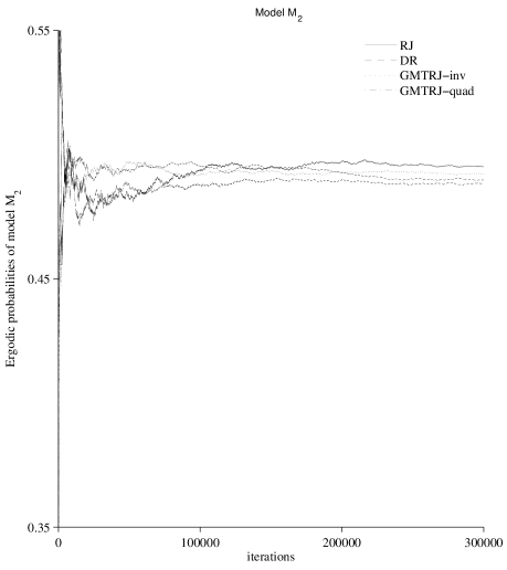
Figure 1: Ergodic posterior model probability of model $\mbox{${\cal M}$}_{2}$ under the logistic regression example. For the multiple-try strategy the size of the trial set is chosen as $k=10$

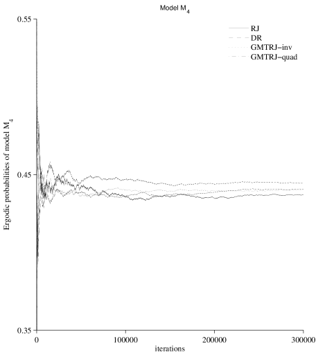
Figure 2: Ergodic posterior model probability of model $\mbox{${\cal M}$}_{4}$ under the logistic regression example. For the multiple-try strategy the size of the trial set is chosen as $k=10$

We observe that 200,000 is more than adequate as number of iterations for the burn-in. Table 4 also shows the acceptance rates of the transdimensional move for all the values of $k$ considered and the corresponding computing time (in seconds) registered at the end of all the iterations (we do not report the results of the GMTRJ-I algorithm since they are quite similar to those of the GMTRJ-inv algorithm). We also observe that the acceptance rate for the RJ algorithm is around 11%, whereas for the GMTRJ-inv and the GMTRJ-quad it is in the range 30-40%, depending on the size of the proposal set. As expected, the DR algorithm shows an higher acceptance rate than the RJ (around 16%). We can also see that the computing time required by the GMTRJ-quad algorithm is less influenced by the number of trial proposals with respect to that required by the GMTRJ-inv algorithm.

		% accepted	CPU time
	RJ	10.77	270.64
	DR	16.28	316.19
$k=10$	GMTRJ-inv	33.97	379.03
	GMTRJ-quad	31.27	358.41
$k=20$	GMTRJ-inv	38.07	443.79
	GMTRJ-quad	34.03	388.76
$k=50$	GMTRJ-inv	40.79	644.16
	GMTRJ-quad	35.64	472.32

Table 4: Acceptance rate and computing time in seconds of the corresponding algorithm for the logistic example

We also compared the algorithms on the basis of the estimated integrated autocorrelation time (IAT), that is proportional to the sum of all-lag autocorrelations between the draws generated by the algorithm of interest and takes into account the permanence in the same model. In order to consider the computational costs, we multiplied the IAT obtained from the output of the different algorithms with the corresponding CPU times (on a Intel Core 2 Duo processor). The results are reported in Table 5.

		$\mbox{${\cal M}$}_{1}$	$\mbox{${\cal M}$}_{2}$	$\mbox{${\cal M}$}_{3}$	$\mbox{${\cal M}$}_{4}$	$\mbox{${\cal M}$}_{5}$
	RJ	7.689	15.405	14.765	12.476	8.322
	DR	7.149	11.177	10.800	8.690	7.327
$k=10$	GMTRJ-I	5.044	8.836	7.450	7.156	5.042
	GMTRJ-inv	5.021	7.840	7.324	6.142	4.798
	GMTRJ-quad	4.771	7.970	6.223	6.607	4.618
$k=20$	GMTRJ-I	5.667	8.970	7.535	7.189	5.993
	GMTRJ-inv	5.795	7.897	7.029	6.581	5.303
	GMTRJ-quad	5.013	7.556	6.535	6.376	4.917
$k=50$	GMTRJ-I	7.672	11.277	9.118	9.286	7.594
	GMTRJ-inv	8.230	10.549	9.883	9.028	7.399
	GMTRJ-quad	6.013	8.685	7.499	7.364	5.902

Table 5: Values (adjusted for the computing time) of the integrated autocorrelation time (IAT) for the logistic example

We observe that there is a consistent gain of efficiency of the GMTRJ algorithms with respect to the RJ and the DR algorithms. Overall, we can see that the proposed GMTRJ-quad algorithm, with $k=10$, outperforms the other algorithms, when the computing time is properly taken into account.

4.3 Latent class analysis

This example is based on the same latent class model and the same data considered by Goodman (1974), which concern the responses to four dichotomous items of a sample of 216 subjects. These items were about the personal feeling toward four situations of role conflict. Here, there are four binary response variables, collected in the vector $\mbox{\boldmath$Y$}=(Y_{1},Y_{2},Y_{3},Y_{4})$, assuming the value 1 if the respondent tends towards universalistic values with respect to the corresponding situation of role conflict and 0 if the respondent tends towards particularistic values (see Goodman, 1974, for a more detailed description of the data).

Parameters of the model are the class weights $\pi_{c}$, collected in the vector $\pi$, and the conditional probabilities of “success” $\lambda_{j|c}$ (i.e., the probability that a subject in latent class $c$ responds by 1 to item $j$, with $j=1,\ldots,4$), where $c=1,\ldots,C$, with $C$ denoting the unknown number of classes. On the basis of these parameters, the probability of the response configuration $\mbox{\boldmath$y$}=(y_{1},y_{2},y_{3},y_{4})$ is given by

$$f(\mbox{\boldmath$y$})=\sum_{c=1}^{C}\pi_{c}\prod_{j=1}^{4}\lambda_{j|c}^{y_{j}}(1-\lambda_{j|c})^{1-y_{j}}.$$

The objective of a Bayesian analysis for the LC model described above is inference for the number of classes $C$ and the parameters $\pi_{c}$ and $\lambda_{j|c}$. A priori, we assumed a Dirichlet distribution for the parameter vector $\mbox{\boldmath$\pi$}\sim D(\delta,\ldots,\delta)$, and independent Beta distributions for the parameters $\lambda_{j|c}\sim Be(\gamma_{1},\gamma_{2})$. Finally, for $C$ we assumed a Uniform distribution between 1 and $C_{\max}$, where $C_{\max}$ is the maximum number of classes.

In order to estimate the posterior distribution of the number of classes and model parameters, we relied on the approach of Richardson and Green (1997), who applied the RJ algorithm to the analysis of finite mixtures of normal densities with an unknown number of components. On the basis of this approach, we adopted an RJ strategy where the moves are restricted to models with one more or one less component.

Moreover, as the estimation algorithm for the LC model is based on the concept of complete data, we also associated to each subject in the sample an allocation variable (or latent variable) $z_{i}$, denoting the subpopulation in which the $i$-th individual belongs to. This variable is equal to $c$ when subject $i$ belongs to latent class $c$. The a priori distribution of each $z_{i}$ depends on the class weights $\pi_{c}$; see also Cappé et al. (2003). Under this formulation, the complete data likelihood has logarithm

$$\ell^{*}(\mbox{\boldmath$\theta$})=\sum_{c}\sum_{\mbox{\scriptsize\boldmath{$y$}}}a_{c\mbox{\scriptsize\boldmath{$y$}}}\log f(c,\hbox{\boldmath$y$}),$$

where $\theta$ is the vector of all model parameters arranged in a suitable way, $a_{c\mbox{\scriptsize\boldmath{$y$}}}$ is the frequency of subjects with latent configuration $c$ and response configuration $y$ and $f(c,\mbox{\boldmath$y$})$ is the manifest distribution

$$f(c,\hbox{\boldmath$y$})=\pi_{c}\prod_{j}\lambda_{j|c}^{y_{j}}(1-\lambda_{j|c})^{(1-y_{j})}.$$

The implemented RJ algorithm is based on two different pairs of dimension-changing moves, split-combine and birth-death, each with probability 0.5, respectively. At every iteration, split-combine or birth-death moves are preceded by a Gibbs move which updates the parameters of the current model, sampling from the full conditional distribution. In particular, the algorithm performs the following steps:

1. Gibbs move: This move aims to update the model parameters given the current number of classes without altering the dimension of the parameters. This can be done through the Gibbs algorithm, sampling from the full conditional distribution. In fact, we have that

   $$\mbox{\boldmath$\pi$}|\cdots\sim D(\delta+n_{1},\ldots,\delta+n_{C}),$$

   where $n_{c}=\#\{i:z_{i}=c\}$, $c=1,\ldots,C$, and where “$\,|\cdots$ ” denotes conditioning on all other variables and parameters. The full conditional for $\lambda_{j|c}$ are

   $$\lambda_{j|c}|\cdots\sim Be\left(\gamma_{1}+\sum_{i}y_{ij}\times I(z_{i}=c),\gamma_{2}+\sum_{i}(1-y_{ij})\times I(z_{i}=c)\right),$$

   where $y_{ij}$ denotes the observed response of subject $i$ to item $j$, with $i=1,\ldots,n$, $j=1,\ldots,4$, and $I(\cdot)$ denotes the indicator function. Finally, for the allocation variable we have

   $$p(z_{i}=c\,|\ldots)\propto\pi_{c}\prod_{j}\lambda_{j|c}^{y_{ij}}(1-\lambda_{j|c})^{1-y_{ij}}.$$

2. Split-combine move: This move aims to split a class into two or combine two classes into one. Suppose that the current state of the chain is $(C,\mbox{\boldmath$\theta$}_{C})$; we first make a random choice between attempting to split or combine with probability 0.5. Obviously, if $C=1$ we always propose a split move whereas if $C=C_{\max}$ we always propose a combine move. The split proposal consists of choosing a class $c^{*}$ at random and splitting it into two new ones, labeled $c_{1}$ and $c_{2}$. The corresponding parameters are split as follows:

   1. $\pi_{c_{1}}=\pi_{c^{*}}\times u$ and $\pi_{c_{2}}=\pi_{c^{*}}\times(1-u)$ with $u\sim Be(\alpha,\beta)$;

   2. $\lambda_{j|c_{1}}\sim Be(\tau\times\lambda_{j|c^{*}},\tau\times(1-\lambda_{j|c^{*}}))$ and $\lambda_{j|c_{2}}\sim Be(\tau\times\lambda_{j|c^{*}},\tau\times(1-\lambda_{j|c^{*}}))$, for $j=1,\ldots,4$, where $\tau$ is a constant that has to be tuned in order to reach an adequate acceptance rate.

   When the split move is accomplished, it remains only to propose the reallocation of those observations with $z_{i}=c^{*}$ between $c_{1}$ and $c_{2}$. The allocation is done on the basis of probabilities computed analogously to the Gibbs allocation.

   In the reverse combine move, a pair of classes $(c_{1},c_{2})$ is picked at random and merged into a new one, $c^{*}$, as follows:

   1. $\pi_{c^{*}}=\pi_{c_{1}}+\pi_{c_{2}}$;

   2. $\lambda_{j|c^{*}}\sim Be(\tau\times\bar{\lambda},\tau\times(1-\bar{\lambda}))$, with $\bar{\lambda}=(\lambda_{j|c_{1}}+\lambda_{j|c_{2}})/2$ for $j=1,\ldots,4$.

   The reallocation of the observations with $z_{i}=c_{1}$ or $z_{i}=c_{2}$ is done by setting $z_{i}=c^{*}$.

   The split move is accepted with probability $\min\{1,A\}$ whereas the combine move is accepted with probability $\min\{1,A^{-1}\}$, where $A$, after some calculation illustrated in B, can be computed as

   $$A = \frac{L^{*}(\hbox{\boldmath$y$}|C+1,\mbox{\boldmath$\theta$}_{C+1})p(\mbox{\boldmath$\theta$}_{C+1}|C+1)}{L^{*}(\hbox{\boldmath$y$}|C,\mbox{\boldmath$\theta$}_{C})p(\mbox{\boldmath$\theta$}_{C}|C)}\times\frac{P_{c}(C+1)}{P_{s}(C)P_{alloc}}$$ (5)

   $$\times \frac{\prod_{j}b_{\tau\times\bar{\lambda},\tau\times(1-\bar{\lambda})}(\lambda_{j|c^{*}})}{b_{\alpha,\beta}(u)\,\prod_{j}b_{\tau\times\lambda_{c^{*}},\tau\times(1-\lambda_{c^{*}})}(\lambda_{j|c_{1}})\;b_{\tau\times\lambda_{c^{*}},\tau\times(1-\lambda_{c^{*}})}(\lambda_{j|c_{2}})}\times|\mbox{\boldmath$J$}_{split}|.$$

   In the above expression, $L^{*}(\hbox{\boldmath$y$}|m,\mbox{\boldmath$\theta$}_{m})$ is the exponential value of the complete data log-likelihood $\ell^{*}(\hbox{\boldmath$y$}|m,\mbox{\boldmath$\theta$}_{m})$. Moreover, $P_{s}(C)$ is the probability of splitting a component when the the current number of classes is $C$, whereas $P_{c}(C+1)$ is the probability of combining two components when the current number of classes is $C+1$. $P_{alloc}$ is the probability that this particular allocation is made, $b_{p,q}(\cdot)$ denotes the $Be(p,q)$ density and $|\mbox{\boldmath$J$}_{split}|$ is the Jacobian of the transformation from $(C,\mbox{\boldmath$\theta$}_{C})$ to $(C+1,\mbox{\boldmath$\theta$}_{C+1})$, which is equal to $\pi_{c^{*}}$.

3. Birth-death move: This move aims to add a new empty class or delete an existing one. In particular, we first propose a birth or a death move along the same lines as above; then, a birth is accomplished by generating a new empty class, that is, a class to which no observation is allocated, denoted by $c^{*}$. To do this we draw $\pi_{c^{*}}$ from a $Be(1,C)$ distribution, where $C$ is the current number of classes, and rescale the existing weights, so that they sum to 1, as $\pi^{\prime}_{c}=\pi_{c}(1-\pi_{c^{*}})$, for $c=1,\ldots,C+1$ with $c\neq c^{*}$. The new parameters $\lambda_{j|c^{*}}$ are drawn, for $j=1,\ldots,4$, from their prior distribution.

   For the death move, a random choice is made between the empty classes; the chosen class is deleted and the remaining class weights are rescaled to sum to 1. The allocation of the $z_{i}$ is unaltered because the class deleted is empty.

   The use of the prior distribution in proposing the new values for $\lambda_{j|c^{*}}$ leads to a simplification of the resulting acceptance probability, $\min\{1,A\}$; after some calculation, $A$ reduces to

   $$A=\frac{\pi_{c^{*}}^{\delta-1}(1-\pi_{c^{*}})^{n+C\delta-C}}{B(C\delta,\delta)}\times\frac{P_{d}(C+1)}{P_{b}(C)}\times\frac{(C+1)}{(C_{0}+1)}\times\frac{1}{g_{1,C}(\pi_{c^{*}})}\times|\mbox{\boldmath$J$}_{birth}|.$$

   Here, the first term is the prior ratio, whereas the likelihood ratio is 1. The remaining terms contain the proposal ratio; in particular, $B(\cdot,\cdot)$ is the Beta function, $C_{0}$ is the number of empty classes and $P_{b}$ and $P_{d}$ are the probability of having a birth and a death, respectively. The Jacobian is computed as $|\mbox{\boldmath$J$}_{birth}|=(1-\pi_{c^{*}})^{C-1}$. The death move is accepted with probability $\min\{1,A^{-1}\}$.

A well-known problem that arises in Bayesian analysis of mixture models is the so-called label switching problem, that is, the non-identifiability of the component due to the invariance of the posterior distribution to the permutations in the parameters labeling. Several solutions have been proposed in the literature, for a review see Jasra et al. (2005). For our illustrative example it is possible to focus solely on the inference about the number of unknown classes, that is invariant to label switching, using relabeling techniques retrospectively by post-processing the RJ output.

We compared the standard RJ algorithm, based on the three steps above, with the proposed GMTRJ algorithm. In particular, this is a situation in which the quadratic approximation of the target distribution cannot be easily computed. In this case, the GMTRJ may again be applied, based on computing the selection probabilities of the proposed trials as a quantity proportional to the incomplete likelihood, corresponding to the manifest distribution of the observable data. The incomplete likelihood does not include the allocation variables $z_{i}$, which have not to be reallocated for each proposed trial. This allows us to easily compute the weighting function, saving much computing time and resulting in an efficient proposal. We refer to this version as the GMTRJ-man algorithm. We also implemented the GMTRJ-inv algorithm based on the weighting function defined in Section 3.2. In general, the GMTRJ scheme consists of choosing at random a single class to split (in the split move) or to add (in the birth move) and the multiple-try strategy is only applied in drawing the parameter values, under the proposed model. The reverse combine and death moves may be easily derived. The comparison also involves the DR algorithm, in a formulation that closely resembles that proposed in Bartolucci et al. (2003). Even in this case, the secondary proposal only consists in drawing the parameter values, under the proposed model.

In order to compare the different algorithms, we ran each Markov chain for 2,000,000 sweeps following a burn-in of 400,000 iterations; moreover, for the parameters of the prior distributions we set $\delta=1$, $\gamma_{1}=\gamma_{2}=1$ and $C_{max}=20$. For the split-combine move we also chose $\alpha=\beta=2$ and $\tau=10$. Finally, for the GMTRJ-inv and GMTRJ-man algorithms, we considered two different sizes of the proposal set $k=5,10$.

Table 6 shows the estimated posterior probabilities of each class for all the algorithms, using $k=5$. We observe that all the algorithms give quite similar posterior probabilities of the number of classes; the two most probable models are those with two and three classes. Table 7 illustrates the proportion of moves accepted, together with the computing time (in seconds) required to run the corresponding algorithm. The plot of the first 20,000 values of $C$ after the burn-in is given in Figure 3. In order to check for stationarity, Figure 4 also shows the plot of the cumulative occupancy fractions for different values of $C$, against the number of sweeps, for the first 1,000,000 iterations. In both figures we considered a fixed number of trials, $k=5$. Finally, Table 8 shows the values of the IAT, so as to measure the autocorrelation of the Markov chain with states corresponding to the models with a number of classes between 2 and 7. As in the previous examples, we report the values corrected for the computing time.

$C$	RJ	DR	GMTRJ-inv	GMTRJ-man
1	0.000	0.000	0.000	0.000
2	0.214	0.211	0.211	0.212
3	0.219	0.217	0.218	0.213
4	0.172	0.174	0.180	0.177
5	0.130	0.131	0.132	0.131
6	0.093	0.092	0.090	0.092
7	0.065	0.063	0.061	0.063
8	0.042	0.042	0.040	0.041
9	0.025	0.027	0.026	0.027
10	0.016	0.016	0.017	0.017
$C\geq 11$	0.024	0.027	0.027	0.027

Table 6: Estimated posterior distribution of the number of classes $C$ for the latent class example. For the multiple-try strategy the size of the trial set is chosen as $k=5$

		% accepted
		split	combine	birth	death	CPU time
	RJ	2.00	1.99	5.33	5.34	2,972.90
	DR	3.23	3.23	7.74	7.74	4,142.00
$k=5$	GMTRJ-inv	5.22	5.18	10.40	10.42	6,263.10
	GMTRJ-man	3.40	3.37	8.45	8.45	3,798.20
$k=10$	GMTRJ-inv	7.28	7.28	11.26	11.31	9,851.50
	GMTRJ-man	4.03	4.03	8.64	8.61	4,242.60

Table 7: Acceptance rate for the latent class example and computing time (in seconds) of the corresponding algorithms

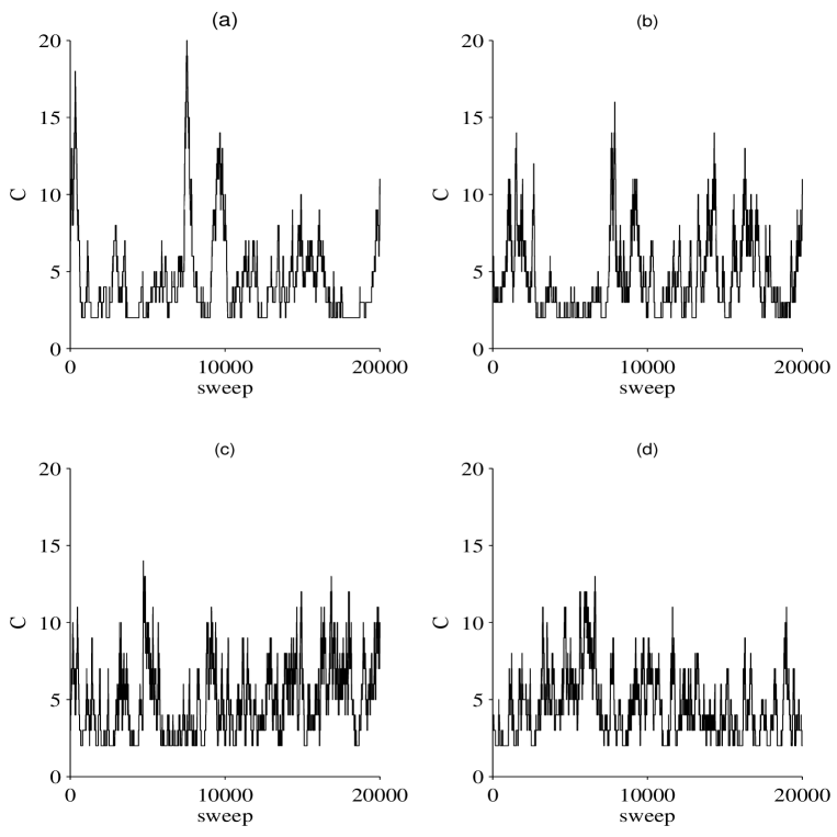
Figure 3: Number of latent classes in the first 20,000 iteration after the burn-in: (a) RJ, (b) DR, (c) GMTRJ-inv with $k=5$, (d) GMTRJ-man with $k=5$

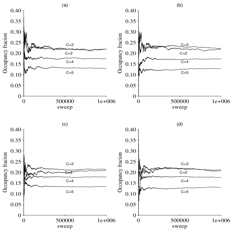
Figure 4: Occupancy fraction for different values of C: (a) RJ, (b) DR, (c) GMTRJ-inv with $k=5$, (d) GMTRJ-man with $k=5$

		Number of classes $C$
		2	3	4	5	6	7
	RJ	473.25	188.32	117.24	105.38	115.04	120.42
	DR	503.10	182.99	105.98	102.28	111.10	118.99
$k=5$	GMTRJ-inv	528.91	205.84	121.50	113.14	125.99	129.94
	GMTRJ-man	271.19	124.97	79.83	68.20	88.09	87.51
$k=10$	GMTRJ-inv	560.58	223.03	134.38	145.14	146.30	147.75
	GMTRJ-man	302.93	139.59	89.17	76.18	98.40	97.75

Table 8: Values (adjusted for the computing time) of the integrated autocorrelation time (IAT) for the latent class example

On the basis of the above results, we conclude that both the DR algorithm and the GMTRJ-inv and GMTRJ-man algorithms have higher acceptance rates than the RJ algorithm. Moreover, all the algorithms mix well over $C$, with few excursions in very high values of $C$ and a quite good mixing (Figure 3). From Figure 4, we observe that for all the algorithms the burn-in is more than adequate to achieve stability of the occupancy fraction. Finally, it is worth noting that, when the size of the trial set increases, the GMTRJ-inv may results in lower efficiency, due to the computational time required. The same can be said for the DR algorithm, whose efficiency, in terms of autocorrelation, is almost equivalent to that of the RJ algorithm, when the computing time is considered. On the other hand, the use of the incomplete likelihood in the computation of the selection probabilities allows the GMTRJ-man to reach quite good performance, even with increasing number of proposal trials. Overall, when the computing time is taken into account, the GMTRJ-man algorithm with $k=5$ outperforms the other algorithms in terms of autocorrelation of the chain.

5 Discussion

We presented an extension of the RJ algorithm, called GMTRJ algorithm, which allows us to explore the different models in a more efficient way. The idea is to exploit the multiple-try paradigm in order to propose a fixed number of transdimensional moves, and then select one of them on the basis of suitable selection probabilities. These probabilities are computed on the basis of a weighting function that can be arbitrary chosen. We illustrated several special cases of the algorithm resulting from this choice. Some of these algorithms may be seen as the corresponding versions, in Bayesian model choice context, of the MTM algorithm introduced by Liu et al. (2000) for Bayesian estimation problems; we termed these algorithms GMTRJ-I and GMTRJ-inv. We also introduced alternative versions of the GMTRJ algorithm, that could be useful in different model selection problems. The first version replaces, in the weighting function, the target distribution with its quadratic approximation, so that the resulting algorithm, that we termed GMTRJ-quad, is more efficient than the standard RJ algorithm, without being much more computationally intensive. We also demonstrated that, when for some variable selection problems the computation of the quadratic approximation is not feasible, it is still possible to derive useful weighting functions that lead to an efficient algorithm.

We illustrated the potential of this approach by a simple example, referred to as the well-known Darwin’s data, and by two more realistic examples. The first concerned the selection of covariates in a logistic regression model. In this example, we compared the performance of the RJ algorithm with the performance of the GMTRJ-I, GMTRJ-inv, and GMTRJ-quad algorithms. We also implemented the DR algorithm introduced by Green and Mira (2001), which has some analogies to the proposed methods. We showed that, in the considered examples, the GMTRJ algorithm outperforms both the RJ and the DR algorithm, with lower stationary autocorrelation of the Markov chain. Moreover, the quadratic approximation allows us to obtain a gain of efficiency with respect to the other algorithms, when the computing time is properly taken into account. The last example involved the estimation of the number of latent classes in an LC model. This is an example in which the computation of the quadratic approximation of the target distribution is not easy to derive. We therefore proposed to use the incomplete likelihood as weighting function; this choice allows us to save much computing time without loss of efficiency. The resulting version of the GMTRJ algorithm was named GMTRJ-man. The results obtained from applying this proposed approach to the LC example yielded good performance.

Further research is necessary to explore different types of weighting function and to better evaluate how this choice affects the efficiency of the resulting algorithm. Moreover, it may be of interest to consider how different extensions of the MTM approach for fixed models proposed in the literature can be applied in the GMTRJ setting. In particular, interesting extensions of the MTM approach are related to different proposal trials (Casarin et al., 2013) or correlated candidates (Qin and Liu, 2001; Craiu and Lemieux, 2007; Martino et al., 2012), which can be selected on the basis of a generic weighting function.

Appendix A Proof of the detailed balance condition

As is common in the MCMC approach, the generated chain has to be reversible and to satisfied the detailed balance condition (Green, 1995). This condition defines a situation of equilibrium in the Markov chain, namely that the probability of being in $\theta$ and moving to $\tilde{\mbox{\boldmath$\theta$}}$ is the same as the probability of being in $\tilde{\mbox{\boldmath$\theta$}}$ and moving back to $\theta$ (see Robert and Casella, 2004, for more details).

In the following theorem we demonstrate that the detailed balance condition holds in the generalized MTM version of the RJ algorithm.

Theorem 1

The GMTRJ algorithm satisfies detailed balance.

The GMTRJ algorithm involves transitions to states of variable dimension, and consequently the detailed balance condition is now written as

$$\pi(m,\mbox{\boldmath$\theta$}_{m})P_{m,{\tilde{m}}}(\mbox{\boldmath$\theta$}_{m},\tilde{\mbox{\boldmath$\theta$}}^{(j)}_{{\tilde{m}}})=\pi({\tilde{m}},\tilde{\mbox{\boldmath$\theta$}}^{(j)}_{{\tilde{m}}})P_{{\tilde{m}},m}(\tilde{\mbox{\boldmath$\theta$}}^{(j)}_{{\tilde{m}}},\mbox{\boldmath$\theta$}_{m})|\mbox{\boldmath$J$}(\mbox{\boldmath$\theta$}_{m},\mbox{\boldmath$u$}^{(j)}_{\tilde{m}})|.$$

where, as above, $\mbox{\boldmath$\theta$}_{m}$ represents the current value of the parameter vector and $\tilde{\mbox{\boldmath$\theta$}}^{(j)}_{\tilde{m}}$ is one of the new parameters proposed for $j=1,\ldots,k$.

Suppose that $\mbox{\boldmath$\theta$}_{m}\neq\tilde{\mbox{\boldmath$\theta$}}^{(j)}_{\tilde{m}}$, noting that $\tilde{\mbox{\boldmath$\theta$}}^{(1)}_{\tilde{m}},\dots,\tilde{\mbox{\boldmath$\theta$}}^{(k)}_{\tilde{m}}$ are exchangeable, it holds that

$$\begin{array}[]{ll}\vspace{2mm}&\pi(m,\mbox{\boldmath$\theta$}_{m})P_{m,{\tilde{m}}}(\mbox{\boldmath$\theta$}_{m},\tilde{\mbox{\boldmath$\theta$}}^{(k)}_{\tilde{m}})=\\ \vspace{2mm}&=k\;\pi(m,\mbox{\boldmath$\theta$}_{m})\;h(m,{\tilde{m}})\;T_{m,\tilde{m}}({\mbox{\boldmath$\theta$}}_{m},\mbox{\boldmath$u$}^{(k)}_{\tilde{m}})\;p_{m,{\tilde{m}}}({\mbox{\boldmath$\theta$}}_{m},\tilde{\mbox{\boldmath$\theta$}}^{(k)}_{\tilde{m}})\\ \vspace{2mm}&\times\displaystyle\int\dots\int T_{m,\tilde{m}}({\mbox{\boldmath$\theta$}}_{m},\mbox{\boldmath$u$}^{(1)}_{\tilde{m}})\dots T_{m,\tilde{m}}({\mbox{\boldmath$\theta$}}_{m},\mbox{\boldmath$u$}^{(k-1)}_{\tilde{m}})\\ \vspace{3mm}&\times\min\left\{\displaystyle 1,\frac{\pi(m,\tilde{\mbox{\boldmath$\theta$}}^{(k)}_{\tilde{m}})\;h({\tilde{m}},m)\;T_{\tilde{m},m}(\tilde{\mbox{\boldmath$\theta$}}^{(k)}_{\tilde{m}},\mbox{\boldmath$u$}_{m})\;p_{{\tilde{m}},m}(\tilde{\mbox{\boldmath$\theta$}}^{(k)}_{\tilde{m}},{\mbox{\boldmath$\theta$}}_{m})}{\pi(m,\mbox{\boldmath$\theta$}_{m})\;h(m,{\tilde{m}})\;T_{m,\tilde{m}}({\mbox{\boldmath$\theta$}}_{m},\mbox{\boldmath$u$}^{(k)}_{\tilde{m}})\;p_{m,{\tilde{m}}}({\mbox{\boldmath$\theta$}}_{m},\tilde{\mbox{\boldmath$\theta$}}^{(k)}_{\tilde{m}})}\;|\mbox{\boldmath$J$}(\mbox{\boldmath$\theta$}_{m},\mbox{\boldmath$u$}^{(k)}_{\tilde{m}})|\right\}\\ \vspace{3mm}&\times T_{{\tilde{m}},m}(\tilde{\mbox{\boldmath$\theta$}}^{(k)}_{\tilde{m}},\bar{\mbox{\boldmath$u$}}^{(1)}_{m})\dots T_{{\tilde{m}},m}(\tilde{\mbox{\boldmath$\theta$}}^{(k)}_{\tilde{m}},\bar{\mbox{\boldmath$u$}}^{(k-1)}_{m})\;d\tilde{\mbox{\boldmath$\theta$}}^{(1)}_{\tilde{m}}\dots d\tilde{\mbox{\boldmath$\theta$}}^{(k-1)}_{\tilde{m}}\;d\bar{\mbox{\boldmath$\theta$}}^{(1)}_{m}\dots d\bar{\mbox{\boldmath$\theta$}}^{(k-1)}_{m}=\\ \vspace{2mm}&=k\;\displaystyle\int\dots\int T_{m,\tilde{m}}({\mbox{\boldmath$\theta$}}_{m},\mbox{\boldmath$u$}^{(1)}_{\tilde{m}})\dots T_{m,\tilde{m}}({\mbox{\boldmath$\theta$}}_{m},\mbox{\boldmath$u$}^{(k-1)}_{\tilde{m}})\\ \vspace{2mm}&\times\min\Big{\{}\pi(m,\mbox{\boldmath$\theta$}_{m})\;h(m,{\tilde{m}})\;T_{m,\tilde{m}}({\mbox{\boldmath$\theta$}}_{m},\mbox{\boldmath$u$}^{(k)}_{\tilde{m}})\;p_{m,{\tilde{m}}}({\mbox{\boldmath$\theta$}}_{m},\tilde{\mbox{\boldmath$\theta$}}^{(k)}_{\tilde{m}}),\\ \vspace{2mm}&\;\;\;\;\;\;\;\;\;\;\;\;\pi(m,\tilde{\mbox{\boldmath$\theta$}}^{(k)}_{\tilde{m}})\;h({\tilde{m}},m)\;T_{\tilde{m},m}(\tilde{\mbox{\boldmath$\theta$}}^{(k)}_{\tilde{m}},\mbox{\boldmath$u$}_{m})\;p_{{\tilde{m}},m}(\tilde{\mbox{\boldmath$\theta$}}^{(k)}_{\tilde{m}},{\mbox{\boldmath$\theta$}}_{m})\;|\mbox{\boldmath$J$}(\mbox{\boldmath$\theta$}_{m},\mbox{\boldmath$u$}^{(k)}_{\tilde{m}})|\Big{\}}\\ \vspace{3mm}&\times T_{{\tilde{m}},m}(\tilde{\mbox{\boldmath$\theta$}}^{(k)}_{\tilde{m}},\bar{\mbox{\boldmath$u$}}^{(1)}_{m})\dots T_{{\tilde{m}},m}(\tilde{\mbox{\boldmath$\theta$}}^{(k)}_{\tilde{m}},\bar{\mbox{\boldmath$u$}}^{(k-1)}_{m})\;d\tilde{\mbox{\boldmath$\theta$}}^{(1)}_{\tilde{m}}\dots d\tilde{\mbox{\boldmath$\theta$}}^{(k-1)}_{\tilde{m}}\;d\bar{\mbox{\boldmath$\theta$}}^{(1)}_{m}\dots d\bar{\mbox{\boldmath$\theta$}}^{(k-1)}_{m}=\\ \vspace{2mm}&=k\;\pi(m,\tilde{\mbox{\boldmath$\theta$}}^{(k)}_{\tilde{m}})\;h({\tilde{m}},m)\;T_{\tilde{m},m}(\tilde{\mbox{\boldmath$\theta$}}^{(k)}_{\tilde{m}},\mbox{\boldmath$u$}_{m})\;p_{{\tilde{m}},m}(\tilde{\mbox{\boldmath$\theta$}}^{(k)}_{\tilde{m}},{\mbox{\boldmath$\theta$}}_{m})\;|\mbox{\boldmath$J$}(\mbox{\boldmath$\theta$}_{m},\mbox{\boldmath$u$}^{(k)}_{\tilde{m}})|\\ \vspace{2mm}&\times\displaystyle\int\dots\int T_{m,\tilde{m}}({\mbox{\boldmath$\theta$}}_{m},\mbox{\boldmath$u$}^{(1)}_{\tilde{m}})\dots T_{m,\tilde{m}}({\mbox{\boldmath$\theta$}}_{m},\mbox{\boldmath$u$}^{(k-1)}_{\tilde{m}})\times\\ \vspace{3mm}&\times\min\left\{1,\frac{\displaystyle\pi(m,\mbox{\boldmath$\theta$}_{m})\;h(m,{\tilde{m}})\;T_{m,\tilde{m}}({\mbox{\boldmath$\theta$}}_{m},\mbox{\boldmath$u$}^{(k)}_{\tilde{m}})\;p_{m,{\tilde{m}}}({\mbox{\boldmath$\theta$}}_{m},\tilde{\mbox{\boldmath$\theta$}}^{(k)}_{\tilde{m}})}{\displaystyle\pi(m,\tilde{\mbox{\boldmath$\theta$}}^{(k)}_{\tilde{m}})\;h({\tilde{m}},m)\;T_{\tilde{m},m}(\tilde{\mbox{\boldmath$\theta$}}^{(k)}_{\tilde{m}},\mbox{\boldmath$u$}_{m})\;p_{{\tilde{m}},m}(\tilde{\mbox{\boldmath$\theta$}}^{(k)}_{\tilde{m}},{\mbox{\boldmath$\theta$}}_{m})}\frac{1}{\displaystyle|\mbox{\boldmath$J$}(\mbox{\boldmath$\theta$}_{m},\mbox{\boldmath$u$}^{(k)}_{\tilde{m}})|}\right\}\\ \vspace{3mm}&\times T_{{\tilde{m}},m}(\tilde{\mbox{\boldmath$\theta$}}^{(k)}_{\tilde{m}},\bar{\mbox{\boldmath$u$}}^{(1)}_{m})\dots T_{{\tilde{m}},m}(\tilde{\mbox{\boldmath$\theta$}}^{(k)}_{\tilde{m}},\bar{\mbox{\boldmath$u$}}^{(k-1)}_{m})\;d\tilde{\mbox{\boldmath$\theta$}}^{(1)}_{\tilde{m}}\dots d\tilde{\mbox{\boldmath$\theta$}}^{(k-1)}_{\tilde{m}}\;d\bar{\mbox{\boldmath$\theta$}}^{(1)}_{m}\dots d\bar{\mbox{\boldmath$\theta$}}^{(k-1)}_{m}=\\ \vspace{2mm}&=\pi({\tilde{m}},\tilde{\mbox{\boldmath$\theta$}}^{(k)}_{{\tilde{m}}})P_{{\tilde{m}},m}(\tilde{\mbox{\boldmath$\theta$}}^{(k)}_{{\tilde{m}}},\mbox{\boldmath$\theta$}_{m})|\mbox{\boldmath$J$}(\mbox{\boldmath$\theta$}_{m},\mbox{\boldmath$u$}^{(k)}_{\tilde{m}})|\end{array}$$

as required. Note that $|\mbox{\boldmath$J$}(\tilde{\mbox{\boldmath$\theta$}}^{(k)}_{\tilde{m}},\mbox{\boldmath$u$}_{m})|=1/|\mbox{\boldmath$J$}(\mbox{\boldmath$\theta$}_{m},\mbox{\boldmath$u$}^{(k)}_{\tilde{m}})|$.

Appendix B Computation of the acceptance probabilities in the split/combine moves

The extended formulation of the acceptance rate of the split/combine move in equation (5), may be expressed as

$$A = \frac{L^{*}(\hbox{\boldmath$y$}|C+1,\mbox{\boldmath$\theta$}_{C+1})p(\mbox{\boldmath$\theta$}_{C+1}|C+1)p(C+1)}{L^{*}(\hbox{\boldmath$y$}|C,\mbox{\boldmath$\theta$}_{C})p(\mbox{\boldmath$\theta$}_{C}|C)p(C)}\!\times\!\frac{(C+1)!}{C!}\!\times\!\frac{P_{c}(C+1)/[(C+1)C/2]}{P_{s}(C)/C}$$

$$\times \frac{1}{P_{alloc}}\!\times\!\frac{\prod_{j}b_{\tau\times\bar{\lambda},\tau\times(1-\bar{\lambda})}(\lambda_{j|c^{*}})}{2\,b_{\alpha,\beta}(u)\,\prod_{j}b_{\tau\times\lambda_{c^{*}},\tau\times(1-\lambda_{c^{*}})}(\lambda_{j|c_{1}})\;b_{\tau\times\lambda_{c^{*}},\tau\times(1-\lambda_{c^{*}})}(\lambda_{j|c_{2}})}\!\times\!|\mbox{\boldmath$J$}_{split}|.$$

In the above expression, the first term represents the product of the likelihood ratio and the prior ratio for the parameters of the model. $P_{s}(C)/C$ and $P_{c}(C+1)/[(C+1)C/2]$ are respectively the probabilities to split a specific class out of $C$ available ones and to combine one of the $(C+1)C/2$ possible pairs of classes. The factorials and the coefficient 2 arise from combinatorial reasoning related to the label switching problem; $P_{alloc}$ is the probability that this particular allocation is made, whereas the last two terms are the product of the proposal ratio and the Jacobian of the transformation from $(C,\mbox{\boldmath$\theta$}_{C})$ to $(C+1,\mbox{\boldmath$\theta$}_{C+1})$.

References

- Azzalini (1985) Azzalini, A., 1985. A class of distributions which includes the normal ones. Scandinavian journal of statistics , 171–178.
- Bartolucci et al. (2003) Bartolucci, F., Mira, L., Scaccia, L., 2003. Answering two biological questions with a latent class model via MCMC applied to capture-recapture data, in: Di Bacco, M., D’Amore, G., Scalfari, F. (Eds.), Applied Bayesian Statistical Studies in Biology and Medicine. Kluwer Academic Publishers, pp. 7–23.
- Bartolucci et al. (2006) Bartolucci, F., Scaccia, L., Mira, A., 2006. Efficient Bayes factor estimation from the reversible jump output. Biometrika 93, 41–52.
- Box and Tiao (1992) Box, G.E.P., Tiao, G.C., 1992. Bayesian inference in statistical analysis. Wiley-Interscience.
- Brooks et al. (2003) Brooks, S., Giudici, P., Roberts, G.O., 2003. Efficient construction of reversible jump Markov chain Monte Carlo proposal distributions. Journal of the Royal Statistical Society, Series B 65, 3–55.
- Cappé et al. (2003) Cappé, O., Robert, C.P., Ryden, T., 2003. Reversible jump, birth-and-death and more general continuous time Markov chain Monte Carlo samplers. Journal of the Royal Statistical Society. Series B 65, 679–700.
- Casarin et al. (2013) Casarin, R., Craiu, R., Leisen, F., 2013. Interacting multiple try algorithms with different proposal distributions. Statistics and Computing 23, 185–200.
- Congdon (2003) Congdon, P., 2003. Applied Bayesian modelling. Wiley.
- Craiu and Lemieux (2007) Craiu, R., Lemieux, C., 2007. Acceleration of the multiple-try metropolis algorithm using antithetic and stratified sampling. Statistics and Computing 17, 109–120.
- Dellaportas et al. (2002) Dellaportas, P., Forster, J., Ntzoufras, I., 2002. On Bayesian model and variable selection using MCMC. Statistics and Computing 12, 27–36.
- Fan et al. (2009) Fan, Y., Peters, G.W., Sisson, S.A., 2009. Automating and evaluating reversible jump MCMC proposal distributions. Statistics and Computing 19, 409–421.
- Fan and Sisson (2011) Fan, Y., Sisson, S.A., 2011. Reversible jump Markov chain Monte Carlo, in: Brooks, S.P., Gelman, A., Jones, G., Meng, X.L. (Eds.), Handbook of Markov Chain Monte Carlo. Chapman and Hall/CRC Press, pp. 69–94.
- Friel and Wyse (2012) Friel, N., Wyse, J., 2012. Estimating the statistical evidence – a review. Statistica Neerlandica 66, 288–308.
- Goodman (1974) Goodman, L., 1974. Exploratory latent structure analysis using both identifiable and unidentifiable models. Biometrika 61, 215–231.
- Green (1995) Green, P.J., 1995. Reversible jump Markov chain Monte Carlo computation and Bayesian model determination. Biometrika 82, 711–732.
- Green (2003) Green, P.J., 2003. Trans-dimensional Markov chain Monte Carlo, in: Green, P., Hjort, N., Richardson, S. (Eds.), Highly structured stochastic systems. Oxford: Oxford University Press, pp. 179–198.
- Green and Mira (2001) Green, P.J., Mira, A., 2001. Delayed rejection in reversible jump Metropolis-Hastings. Biometrika 88, 1035–1053.
- Han and Carlin (2000) Han, C., Carlin, B.P., 2000. Markov chain Monte Carlo methods for computing Bayes factors: a comparative review. Journal of the American Statistical Association 96, 1122–1132.
- Hastie (2005) Hastie, D., 2005. Towards automatic reversible jump Markov chain Monte Carlo. Ph.D. thesis. University of Bristol.
- Hastie and Green (2012) Hastie, D., Green, P.J., 2012. Model choice using reversible jump Markov Chain Monte Carlo. Statistica Neerlandica 66, 309–338.
- Hastings (1970) Hastings, W.K., 1970. Monte Carlo sampling methods using Markov chains and their applications. Journal of Chemical Physics 21, 1087–1091.
- Jasra et al. (2005) Jasra, A., Holmes, C.C., Stephens, D.A., 2005. MCMC and the label switching problem in Bayesian mixture models. Statistical Science 20, 50–67.
- Jasra et al. (2007) Jasra, A., Stephens, D.A., Holmes, C.C., 2007. Population-based reversible jump Markov Chain Monte Carlo. Biometrika 94, 787–807.
- Liu et al. (2000) Liu, J.S., Liang, F., Wong, W.H., 2000. The Multiple-try Method and local optimization in Metropolis sampling. Journal of American Statistical Association 95, 121–134.
- Liu et al. (2011) Liu, R.Y., Tao, J., Shi, N.Z., He, X., 2011. Bayesian analysis of the patterns of biological susceptibility via reversible jump MCMC sampling. Computational Statistics & Data Analysis 55, 1498 – 1508.
- Lopes and West (2004) Lopes, H.F., West, M., 2004. Bayesian model assessment in factor analysis. Statistica Sinica 14, 41–67.
- Lunn et al. (2009) Lunn, J., Best, N., Whittaker, J., 2009. Generic reversible jump MCMC using graphical models. Statistics and Computing 19, 395–408.
- Martino et al. (2012) Martino, L., Olmo, V.P.D., Read, J., 2012. A multi-point metropolis scheme with generic weight functions. Statistics & Probability Letters 82, 1445 – 1453.
- Metropolis et al. (1953) Metropolis, N., Rosenbluth, A.W., Rosenbluth, M.N., Teller, A.H., Teller, E., 1953. Equation of state calculations by fast computing machine. Journal of Chemical Physics 21, 1087–1091.
- van der Meulen et al. (2013) van der Meulen, F., Schauer, M., van Zanten, H., 2013. Reversible jump MCMC for nonparametric drift estimation for diffusion processes. Computational Statistics & Data Analysis in press.
- Pandolfi et al. (2010) Pandolfi, S., Bartolucci, F., Friel, N., 2010. A generalization of the Multiple-try Metropolis algorithm for Bayesian estimation and model selection, in: Proceedings of the International Conference on Artificial Intelligence and Statistics (AISTATS 2010), Chia Laguna Resort, Sardinia, Italy. pp. 581–588.
- Qin and Liu (2001) Qin, Z.S., Liu, J.S., 2001. Multipoint metropolis method with application to hybrid Monte Carlo. Journal of Computational Physics 172, 827 – 840.
- Richardson and Green (1997) Richardson, S., Green, P., 1997. On Bayesian analysis of mixture with an unknown number of components. Journal of the Royal Statistical Society, Series B 59, 731–792.
- Robert and Casella (2004) Robert, C.P., Casella, G., 2004. Monte Carlo statistical methods. Springer, New-York.
- Spiegelhalter et al. (1996) Spiegelhalter, D., Thomas, A., Best, N., Gilks, W., 1996. Bugs 0.5: Bayesian inference using gibbs sampling manual (version ii). MRC Biostatistics Unit, Institute of Public Health, Cambridge, UK .
- Stephens (2000) Stephens, M., 2000. Bayesian analysis of mixture models with an unknown number of components - an alternative to reversible jump methods. The Annals of Statistics 28, 40–74.
- Tierney and Mira (1999) Tierney, L., Mira, A., 1999. Some adaptive Monte Carlo methods for Bayesian inference. Statistics in Medicine 18, 2507–2515.
- Zhang et al. (2004) Zhang, Z., Chan, K., Wu, Y., Chen, C., 2004. Learning a multivariate gaussian mixture model with the reversible jump MCMC algorithm. Statistics and Computing 14, 343–355.